y response variable x 1, x 2,, x k -- a set of explanatory variables

Transcription

1 11. Multiple Regression and Correlation y response variable x 1, x 2,, x k -- a set of explanatory variables In this chapter, all variables are assumed to be quantitative. Chapters show how to incorporate categorical variables also in a regression model. Multiple regression equation (population): E(y) = a + b 1 x 1 + b 2 x b k x k

2 Parameter Interpretation a = E(y) when x 1 = x 2 = = x k = 0. b 1, b 2,, b k are called partial regression coefficients. Controlling for other predictors in model, there is a linear relationship between E(y) and x 1 with slope b 1. i.e., consider case of k = 2 explanatory variables, E(y) = a + b 1 x 1 + b 2 x 2 If x 1 goes up 1 unit with x 2 held constant, the change in E(y) is [a + b 1 (x 1 + 1) + b 2 x 2 ] [a + b 1 x 1 + b 2 x 2 ] = b 1.

3

4 Prediction equation With sample data, software finds least squares estimates of parameters by minimizing SSE = sum of squared prediction errors (residuals) = (observed y predicted y) 2 Denote the sample prediction equation by ˆ k k y a b x b x b x

5 Example: Mental impairment study y = mental impairment (summarizes extent of psychiatric symptoms, including aspects of anxiety and depression, based on questions in Health opinion survey with possible responses hardly ever, sometimes, often) Ranged from 17 to 41 in sample, mean = 27, s = 5. x 1 = life events score (composite measure of number and severity of life events in previous 3 years) Ranges from 0 to 100, sample mean = 44, s = 23 x 2 = socioeconomic status (composite index based on occupation, income, and education) Ranges from 0 to 100, sample mean = 57, s = 25 Data (n = 40) at and p. 327 of text

6 Other explanatory variables in study (not used here) include age, marital status, gender, race. Bivariate regression analyses give prediction equations: Correlation matrix yˆ x yˆ x 1 2

7 Prediction equation for multiple regression analysis is: yˆ x x 1 2

8 Predicted mental impairment: increases by for each 1-unit increase in life events, controlling for (at a fixed value of) SES. decreases by for each 1-unit increase in SES, controlling for life events. (e.g., decreases by 9.7 when SES goes from minimum of 0 to maximum of 100, which is relatively large since sample standard deviation of y is 5)

9 Can we compare the estimated partial regression coefficients to determine which explanatory variable is most important in the predictions? These estimates are unstandardized and so depend on units of measurement. Standardized coefficients presented in multiple regression output refer to partial effect of a standard deviation increase in a predictor, keeping other predictors constant. (Sec. 11.8). In bivariate regression, standardized coefficient = correlation. In multiple regression, stand. coeff. relates algebraically to partial correlations (Sec. 11.7). We skip or only briefly cover Sec. 11.7, 11.8 (lack of time), but I ve included notes at end of this chapter on these topics if you want to see how these work.

10 Predicted values and residuals One subject in the data file has y = 33, x 1 = 45 (near mean), x 2 = 55 (near mean) This subject has predicted mental impairment yˆ (45) 0.097(55) 27.5 (near mean) The prediction error (residual) is = 5.5 i.e., this person has mental impairment 5.5 higher than predicted given his/her values of life events, SES. SSE = smaller than SSE for either bivariate model or for any other linear equation with predictors x 1, x 2.

11 Comments Partial effects in multiple regression refer to controlling other variables in model, so differ from effects in bivariate models, which ignore all other variables. Partial effect of x 1 (controlling for x 2 ) is same as bivariate effect of x 1 when correlation = 0 between x 1 and x 2 (as is true in most designed experiments). Partial effect of a predictor in this multiple regression model is identical at all fixed values of other predictors in model Example: At x 2 = 0, At x 2 = 100, yˆ x x 1 2 yˆ x 0.097(0) x 1 1 yˆ x 0.097(100) x 1 1

12 This parallelism means that this model assumes no interaction between predictors in their effects on y. (i.e., effect of x 1 does not depend on value of x 2 ) Model is inadequate if, in reality (insert graph) The model E(y) = a + b 1 x 1 + b 2 x b k x k is equivalently expressed as y = a + b 1 x 1 + b 2 x b k x k + where = y E(y) = error having E( ) = 0 is population analog of residual e = y predicted y.

13 Graphics for multiple regression Scatterplot matrix: Scatterplot for each pair of variables

14 Partial regression plots: One plot for each predictor, shows its partial effect controlling for other predictors Example: With two predictors, show partial effect of x 1 on y (i.e., controlling for x 2 ) by using residuals after Regressing y on x 2 Regressing x 1 on x 2 Partial regression plot is a scatterplot with residuals from regressing y on x 2 on vertical axis and residuals from regressing x 1 on x 2 on horizontal axis. The prediction equation for these points has the same slope as the effect of x 1 in the prediction equation for the multiple regression model.

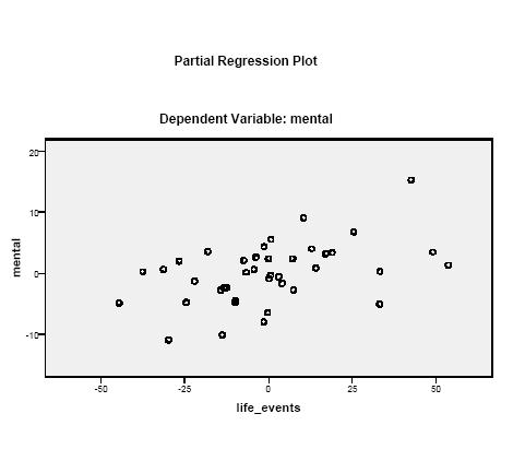
15

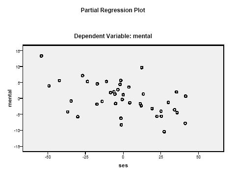
16

17 Multiple correlation and R 2 How well do the explanatory variables in the model predict y, using the prediction equation? The multiple correlation, denoted by R, is the correlation between the observed y-values and predicted values yˆ a b1 x1 b2 x2... bkxk from the prediction equation. i.e., it is the ordinary correlation between y and an artificial variable whose values for the n subjects in the sample are the predicted values from the prediction equation.

18 Example: Mental impairment predicted by life events and SES The multiple correlation is the correlation between the n = 40 pairs of values of observed y and predicted y values: Subject y Predicted y yˆ x x = (46) 0.097(84) = (39) 0.097(97) = (27) 0.097(24) Software reports R = 0.58 (bivariate correlations with y were 0.37 for x 1, for x 2 )

19 The coefficient of multiple determination R 2 is the proportional reduction in error obtained by using the prediction equation to predict y instead of using to predict y y R 2 TSS SSE ( y y) ( y yˆ ) 2 TSS ( y y) 2 2 Example: Predictor TSS SSE R 2 x x x 1 and x For the multiple regression model, R TSS SSE ( y y) ( y yˆ ) TSS ( y y)

20 Software provides an ANOVA table with the sums of squares used in R-squared and a Model Summary table with values of R and R-squared.

21 R 2 = 0.34, so there is a 34% reduction in error when we use life events and SES together to predict mental impairment (via the prediction equation), compared to using y to predict mental impairment. This is sometimes expressed as 34% of the variation in mental impairment is explained by life events and SES The multiple correlation is R = = the correlation between the 40 values of y and the 40 corresponding predicted y-values from the prediction equation for the multiple regression model.

22 0 R 2 1 Properties of R and R 2 2 so 0 R 1 (i.e., it can t be negative) R R The larger their values, the better the set of explanatory variables predict y R 2 = 1 when observed y = predicted y, so SSE = 0 R 2 = 0 when all predicted y = so TSS = SSE. When this happens, b 1 = b 2 = = b k = 0 and the correlation r = 0 between y and each x predictor. R 2 cannot decrease when predictors added to model With single predictor, R 2 = r 2, R = r y

23 The numerator of R 2, which is TSS SSE, is called the regression sum of squares. This represents the variability in y explained by the model. R 2 is additive (i.e., it equals the sum of r 2 values from bivariate regressions of y with each x) when each pair of explanatory variables is uncorrelated; this is true in many designed experiments, but we don t expect it in observational studies. Sample R 2 tends to be a biased estimate (upwards) of population value of R 2, more so for small n (e.g., extreme case -- consider n = 2 in bivariate regression!) Software also reports adjusted R 2, a less biased estimate (p. 366, Exer )

24 Inference for multiple regression Based on assumptions Model E(y) = a + b 1 x 1 + b 2 x b k x k is (nearly) correct Population conditional distribution of y is normal, at each combination of predictor values Standard deviation σ of conditional dist. of responses on y is same at each combination of predictor values (The estimate s of σ is the square root of MSE. It is what SPSS calls Std. error of the estimate in the Model Summary table.) Sample is randomly selected Two-sided inference about b parameters is robust to normality and common σ assumptions

25 Collective influence of explanatory var s To test whether explanatory variables collectively have effect on y, we test H 0 : 1 = 2 = = k = 0 (i.e., y independent of all the explanatory variables) H a : At least one i 0 (at least one explanatory variable has an effect on y, controlling for the others in the model) Equivalent to testing H 0 : population multiple correlation = 0 (or popul. R 2 = 0) vs. H a : population multiple correlation > 0

26 Test statistic (with k explanatory variables) F 2 R / k 2 (1 R ) /[ n ( k 1)] When H 0 true, F values follow the F distribution (R. A. Fisher) Larger R gives larger F test statistic, more evidence against null hypothesis. Since larger F gives stronger evidence against null, P-value = right-tail probability above observed value

27 Properties of F distribution F can take only nonnegative values Distribution is skewed right Mean is approximately equal to 1 (closer to 1 for large n) Exact shape depends on two df values: df 1 = k (number of explanatory variables in model) df 2 = n (k + 1) (sample size no. model parameters) F tables report F-scores for right-tail probabilities such as 0.05, 0.01, (one table for each tail prob.)

28 Example: Is mental impairment independent of life events and SES? H 0 : 1 = 2 = 0 (i.e., y independent of x 1 and x 2 ) H a : 1 0 or 2 0 or both Test statistic F 2 R / k 0.339/ 2 2 (1 R ) /[ n ( k 1)] ( ) /[40 (2 1)] 9.5 df 1 = 2, df 2 = 37, P-value = (i.e., P < 0.001) (From F tables, F = 3.25 has P-value = 0.05 F = 8.37 has P-value = 0.001)

29 Software provides ANOVA table with result of F test about all regression parameters

30 There is very strong evidence that at least one of the explanatory variables is associated with mental impairment. Alternatively, can calculate F as ratio of mean squares from the ANOVA table. Example: F = /20.76 = 9.5

31 Inferences for individual regression coefficients (Need all predictors in model?) To test partial effect of x i controlling for the other explan. var s in model, test H 0 : i = 0 using test stat. t = (b i 0)/se, df = n - (k + 1) which is df 2 from the F test (and in df column of ANOVA table in Residual row) CI for i has form b i ± t(se), with t-score from t-table also having df = n - (k + 1), for the desired confidence level Software provides estimates, standard errors, t test statistics, P-values for tests (2-sided by default)

32 In SPSS, check confidence intervals under Statistics in Linear regression dialog box to get CI s for regression parameters (95% by default)

33 Example: Effect of SES on mental impairment, controlling for life events H 0 : 2 = 0, H a : 2 0 Test statistic t = b 2 /se = /0.029 = -3.35, df = n - (k + 1) = 40 3 = 37. Software reports P-value = Conclude there is very strong evidence that SES has a negative effect on mental impairment, controlling for life events. (We would reject H 0 at standard significance levels, such as 0.05.) Likewise for test of H 0 : 1 = 0 (P-value = 0.003), but life events has positive effect on mental impairment, controlling for SES.

34 A 95% CI for 2 is b 2 ± t(se), which is ± 2.03(0.029), or (-0.16, -0.04) This does not contain 0, in agreement with rejecting H 0 for two-sided H a at 0.05 significance level Perhaps simpler to interpret corresponding CI of (-16, -4) for the change in mean mental impairment for an increase of 100 units in SES (from minimum of 0 to maximum of 100). (relatively wide CI because of relatively small n = 40) Why bother with F test? Why not go right to the t tests?

35 A caution: Overlapping variables (multicollinearity) It is possible to get a small P-value in F test of H 0 : 1 = 2 = = k = 0 yet not get a small P-value for any of the t tests of individual H 0 : i = 0 Likewise, it is possible to get a small P-value in a bivariate test for a predictor but not for its partial test controlling for other variables. This happens when the partial variability explained uniquely by a predictor is small. (i.e., each x i can be predicted well using the other predictors) (picture) Example (purposely absurd): y = height x 1 = length of right leg, x 2 = length of left leg

36 When multicollinearity occurs, se values for individual b i may be large (and individual t statistics not significant) R 2 may be nearly as large when drop some predictors from model It is advisable to simplify the model by dropping some nearly redundant explanatory variables. There is a variance inflation factor (VIF) diagnostic for describing extent of multicollinearity (text p. 456).

37 Modeling interaction between predictors Recall that the multiple regression model E(y) = a + b 1 x 1 + b 2 x b k x k assumes the partial slope relating E(y) to each x i is the same at all values of other predictors (i.e., assumes no interaction between pairs of predictors in their effects on y) (recall picture showing parallelism, in context of ex.) For a model allowing interaction between x 1 and x 2 the effect of x 1 may change as x 2 changes.

38 Simplest interaction model: Introduce cross product terms for predictors Ex: k = 2 explanatory var s: E(y) = a + b 1 x 1 + b 2 x 2 + b 3 (x 1 x 2 ) is special case of the multiple regression model E(y) = a + b 1 x 1 + b 2 x 2 + b 3 x 3 with x 3 = x 1 x 2 (create x 3 in transform menu with compute variable option in SPSS) Example: For mental impairment data, R 2 goes up from (without interaction) to 0.358, and we get ŷ = x x x 1 x 2

39 SPSS output for interaction model (need more decimal places!)

40 Fixed x 2 Prediction equation for y and x x (0) x 1 (0) = x x (50) x 1 (50) = x x (100) x 1 (100) = x 1 The higher the value of SES, the weaker the relationship between y = mental impairment and x 1 = life events (plausible for these variables)

41 Comments about interaction model Note that E(y) = a + b 1 x 1 + b 2 x 2 + b 3 x 1 x 2 = (a + b 2 x 2 ) + (b 1 + b 3 x 2 )x 1 i.e, E(y) is a linear function of x 1 E(y) = (constant with respect to x 1 ) + (coeff. of x 1 )x 1 where coefficient of x 1 is (b 1 + b 3 x 2 ). For fixed x 2 the slope of the relationship between E(y) and x 1 depends on the value of x 2. To model interaction with k > 2 explanatory variables, take cross product for each pair; e.g., k = 3: E(y) = a + b 1 x 1 + b 2 x 2 + b 3 x 3 + b 4 x 1 x 2 + b 5 x 1 x 3 + b 6 x 2 x 3

42 To test H 0 : no interaction in model E(y) = a + b 1 x 1 + b 2 x 2 + b 3 x 1 x 2, test H 0 : b 3 = 0 using test statistic t = b 3 /se. Example: t = / = -0.67, df = n 4 = 36. P-value = 0.51 for H a : b 3 0 Insufficient evidence to conclude that interaction exists. (It is significant for the entire data set, with n > 1000) With several predictors, often some interaction terms are needed but not others. E.g., could end up using model such as E(y) = a + b 1 x 1 + b 2 x 2 + b 3 x 3 + b 4 x 1 x 2 Be careful not to misinterpret main effect terms when there is interaction between them in the model.

43 Comparing two regression models How to test whether a model gives a better fit than a simpler model containing only a subset of the predictors? Example: Compare E(y) = a + b 1 x 1 + b 2 x 2 + b 3 x 3 + b 4 x 1 x 2 + b 5 x 1 x 3 + b 6 x 2 x 3 to E(y) = a + b 1 x 1 + b 2 x 2 + b 3 x 3 to test H 0 : no interaction by testing H 0 : b 4 = b 5 = b 6 = 0.

44 An F test compares the models by comparing their SSE values, or equivalently, their R 2 values. The more complex ( complete ) model is better if its SSE is sufficiently smaller (or equivalently if its R 2 value is sufficiently larger) than the SSE (or R 2 ) value for the simpler ( reduced ) model. Denote the SSE values for the complete and reduced models by SSE c and SSE r. Denote the R 2 values by R 2 c and R 2 r. The test statistic for comparing the models is F ( SSE SSE ) / df ( R R ) / df 2 2 r c 1 c r 1 2 c / 2 (1 c) / 2 SSE df R df df 1 = number of extra parameters in complete model, df 2 = n-(k+1) = df 2 for F test that all b terms in complete model = 0 (e.g., df 2 = n 7 for model above)

45 Example: Mental impairment study (n = 40) Reduced model: E(y) = a + b 1 x 1 + b 2 x 2 for x 1 = life events score, x 2 = SES Complete model: E(y) = a + b 1 x 1 + b 2 x 2 + b 3 x 3 with x 3 = religious attendance (number of times subject attended religious service in past year) R 2 r = 0.339, R 2 c = Test comparing models has H 0 : b 3 = 0.

46 Test statistic F 2 2 ( Rc Rr ) / df1 ( ) /1 2 Rc df (1 ) / ( ) /(40 4) with df 1 = 1, df 2 = 36. P-value = We cannot reject H 0 at the usual significance levels (such as 0.05). The simpler model is adequate. Note: Since only one parameter in null hypo., the F test statistic is the square of t = b 3 /se for testing H 0 : b 3 = 0. The t test also gives P-value = 0.51, for H a : b 3 0

47 Partial Correlation Used to describe association between y and an explanatory variable, while controlling for the other explanatory variables in the model Notation: r yx 1. x 2 denotes the partial correlation between y and x 1 while controlling for x 2. Formula in text (p. 347), which we ll skip, focusing on interpretation and letting software do the calculation. ( correlate on Analyze menu has a partial correlation option)

48 Properties of partial correlation Falls between -1 and +1. The larger the absolute value, the stronger the association, controlling for the other variables Does not depend on units of measurement Has same sign as corresponding partial slope in the prediction equation Can regard r yx as approximating the ordinary 1. x 2 correlation between y and x 1 at a fixed value of x 2. Equals ordinary correlation found for data points in the corresponding partial regression plot Squared partial correlation has a proportional reduction in error (PRE) interpretation for predicting y using that predictor, controlling for other explan. var s in model.

49 Example: Mental impairment as function of life events and SES The ordinary correlations are: between y and life events between y and SES The partial correlations are: between y and life events, controlling for SES between y and SES, controlling for life events

50 Notes: Since partial correlation = between y and life events, controlling for SES, and since (0.463) 2 = 0.21, Controlling for SES, 21% of the variation in mental impairment is explained by life events. or Of the variability in mental impairment unexplained by SES, 21% is explained by life events.

51 Test of H 0 : population partial correlation = 0 is equivalent to t test of H 0 : population partial slope = 0 For the corresponding regression parameter. e.g., model E(y) = a + b 1 x 1 + b 2 x 2 + b 3 x 3 H 0 : population partial correlation = 0 between y and x 2 controlling for x 1 and x 3 is equivalent to test of H 0 : b 2 = 0

52 Standardized Regression Coefficients Recall for a bivariate model, the correlation is a standardized slope, reflecting what the slope would be if x and y had equal standard dev s. In multiple regression, there are also standardized regression coefficients that describe what the partial regression coefficients would equal if all variables had the same standard deviation. Def: The standardized regression coefficient for an explanatory variable represents the change in the mean of y (in y std. dev s) for a 1-std.-dev. increase in that variable, controlling for the other explanatory variables in the model

53 r = b(s x /s y ) (bivariate) generalizes to b 1 * = b 1 (s x1 / s y ) b 2 * = b 2 (s x2 / s y ), etc. Properties of standardized regression coeff s: Same sign as unstandardized coefficients, but do not depend on units of measurement Represent what the partial slopes would be if the standard deviations were equal Equals 0 when unstandardized coeff. = 0, so a new test is not needed about significance SPSS reports in same table as unstandardized coefficients

54 Example: Mental impairment by life events and SES We found unstandardized equation yˆ x x 1 2 Standard deviations s y = 5.5, s x1 = 22.6, s x2 = 25.3 The standardized coefficient for the effect of life events is b 1 * = 0.103(22.6/5.5) = Likewise b 2 * = -0.45

55 We estimate that E(y) increases by 0.43 standard deviations for a 1 std. dev. increase in life events, controlling for SES. Note: An alternative form for prediction equations uses standardized regression coefficients as coefficients of standardized variables (text, p. 352)

56 Some multiple regression review questions Predicted cost = (food) (décor) (service) a. The correct interpretation of the estimated regression coefficient for décor is: for a 1-point increase in the décor score, the predicted cost of dining increases by $1.58 b. Décor is the most important predictor c. Décor has a positive correlation with cost d. Ignoring other predictors, it is impossible that décor could have a negative correlation with cost e. The t statistic for testing the partial effect of décor against the alternative of a positive effect could have a P-value above 0.50 f. None of the above

57 (T/F) For the multiple regression model with two predictors, if the correlation between x 1 and y is 0.50 and the correlation between x 2 and y is 0.50, it is possible that the multiple correlation R = For the previous exercise in which case would you expect R 2 to be larger: when the correlation between x 1 and x 2 is 0, or when it is 1.0? (T/F) For every F test, there is always an equivalent t test. Explain with an example what it means for there to be (a) no interaction, (b) interaction between two quantitative explanatory variables in their effects on a quantitative response variable. Give an example of interaction when the three variables are categorical (see back in Chap. 10, p. 12 of notes).

58 Why do we need multiple regression? Why not just do a set of bivariate regressions, one for each explanatory variable? Approximately what value do you expect to see for a F test statistic when a null hypothesis is true? (T/F) If you get a small P-value in the F test that all regression coefficients = 0, then the P-value will be small in at least one of the t tests for the individual regression coefficients. Why do we need the F (chi-squared) distribution? Why can t we use the t (normal) distribution for all hypotheses involving quantitative (categorical) var s? What is the connection between (a) t and F, (b) z and chi-squared?