(quantitative or categorical variables) Numerical descriptions of center, variability, position (quantitative variables)

Transcription

1 3. Descriptive Statistics Describing data with tables and graphs (quantitative or categorical variables) Numerical descriptions of center, variability, position (quantitative variables) Bivariate descriptions (In practice, most studies have several variables)

2 1. Tables and Graphs Frequency distribution: ib ti Lists possible values of variable and number of times each occurs Example: Student survey (n = 60) aa/social/data political l ideology measured as ordinal variable with 1 = very liberal, 4 = moderate, 7 = very conservative

3

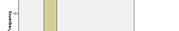
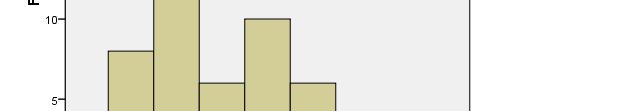
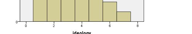
4 Histogram: Bar graph of frequencies or percentages

5 Shapes of histograms Bell-shaped (IQ, SAT, political ideology in all U.S. ) Skewed right (annual income, no. times arrested) Skewed left (score on easy exam) Bimodal (polarized opinions) Ex. GSS data on sex before marriage in Exercise 3.73: always wrong, almost always wrong, wrong only sometimes, not wrong at all category counts 238, 79, 157, 409

6 Stem-and-leaf plot Example: Exam scores (n = 40 students) Stem Leaf

7 2.Numerical descriptions Let y denote a quantitative variable, with observations y 1, y 2, y 3,, y n a. Describing the center Median: Middle measurement of ordered sample y + y + + y Σy = = n n Mean: n i y

8 Example: Annual per capita carbon dioxide emissions (metric tons) for n = 8 largest nations in population size Bangladesh 0.3, Brazil 1.8, China 2.3, India 1.2, Indonesia 1.4, Pakistan 0.7, Russia 9.9, U.S Ordered sample: Median = Mean = y

9 Example: Annual per capita carbon dioxide emissions (metric tons) for n = 8 largest nations in population size Bangladesh 0.3, Brazil 1.8, China 2.3, India 1.2, Indonesia 1.4, Pakistan 0.7, Russia 9.9, U.S Ordered sample: 0.3, 0.7, 1.2, 1.4, 1.8, 2.3, 9.9, 20.1 Median = Mean = y

10 Example: Annual per capita carbon dioxide emissions (metric tons) for n = 8 largest nations in population size Bangladesh 0.3, Brazil 1.8, China 2.3, India 1.2, Indonesia 1.4, Pakistan 0.7, Russia 9.9, U.S Ordered sample: 0.3, 0.7, 1.2, 1.4, 1.8, 2.3, 9.9, 20.1 Median = ( )/2 = 1.6 Mean = ( )/8 = 4.7 y

11 Properties of mean and median For symmetric distributions, mean = median For skewed distributions, mean is drawn in direction of longer tail, relative to median Mean valid for interval scales, median for interval or ordinal scales Mean sensitive to outliers (median often preferred for highly skewed distributions) When distribution symmetric or mildly skewed or discrete with few values, mean preferred because uses numerical values of observations

12 Examples: NY Yankees baseball team in 2006 mean salary = $7.0 million median salary = $2.9 million How possible? Direction of skew? Give an example for which you would expect mean < median

13 b. Describing variability Range: Difference between largest and smallest observations (but highly sensitive to outliers, insensitive to shape) Standard deviation: A typical distance from the mean The deviation of observation i from the mean is yi y

14 The variance of the n observations is s Σ ( y y ) 2 ( y y ) ( y y ) 2 2 i 1 n = = n 1 n 1 The standard deviation s is the square root of the variance, s = s 2

15 Example: Political ideology For those in the student sample who attend religious services at least once a week (n = 9 of the 60), y = 2, 3, 7, 5, 6, 7, 5, 6, 4 y = s 5.0, (2 5) + (3 5) (4 5) 24 = = = s = 3.0 = F ti l ( 60) 3 0 t d d d i ti 1 6 For entire sample (n = 60), mean = 3.0, standard deviation = 1.6, tends to have similar variability but be more liberal

16 Properties of the standard deviation: s 0, and only equals 0 if all observations are equal s increases with the amount of variation around the mean Division by n - 1 (not n) is due to technical reasons (later) s depends on the units of the data (e.g. measure euro vs $) Like mean, affected by outliers Empirical rule: If distribution approx. bell-shaped, about 68% of data within 1 std. dev. of mean about 95% of data within 2 std. dev. of mean all or nearly all data within 3 std. dev. of mean

17 Example: SAT with mean = 500, s = 100 (sketch picture summarizing data) Example: y = number of close friends you have Recent GSS data has mean 7, s = 11 Probably highly skewed: right or left? Empirical rule fails; in fact, median = 5, mode=4 Example: y = selling price of home in Syracuse, NY. If mean = $130,000, which is realistic? s=0, s=1000, s= 50,000, s = 1,000,000

18 c. Measures of position p th percentile: p percent of observations below it, (100 - p)% above it. p = 50: median p = 25: lower quartile (LQ) p = 75: upper quartile (UQ) Interquartile range IQR = UQ - LQ

19 Quartiles portrayed graphically by box plots (John Tukey 1977) Example: weekly TV watching for n=60 students, t 3 outliers

20 Box plots have box from LQ to UQ, with median marked. They yportray a five- number summary of the data: Minimum, LQ, Median, UQ, Maximum with outliers identified separately Outlier = observation falling below LQ 1.5(IQR) or above UQ + 1.5(IQR) E If LQ 2 UQ 10 th IQR 8 d Ex. If LQ = 2, UQ = 10, then IQR = 8 and outliers above (8) = 22

21 Bivariate description Usually we want to study associations between two or more variables (e.g., how does number of close friends depend on gender, income, education, age, working status, rural/urban, religiosity ) Response variable: the outcome variable Explanatory variable: defines groups to compare Ex.: number of close friends is a response variable, while gender, income, are explanatory variables Response = dependent variable Response = dependent variable Explanatory = independent variable

22 Summarizing associations: Categorical var s: show data using contingency tables Quantitative var s: show data using scatterplots Mixture of categorical var. and quantitative var. (e.g., number of close friends and gender) can give numerical summaries (mean, standard deviation) or side-by-side box plots for the groups Ex. General Social Survey (GSS) data Men: mean = 7.0, s = 8.4 Women: mean = 5.9, s = Shape? Inference questions for later chapters?

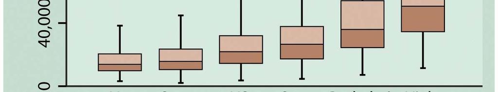
23 Example: Income by highest degree

24 Contingency Tables Cross classifications of categorical variables in which rows (typically) represent categories of explanatory variable and columns represent categories of response variable. Numbers in cells of the table give the numbers of individuals at the corresponding combination of levels of the two variables

25 Happiness and Family Income (GSS 2006 data) Happiness Income Very Pretty Not too Total Above Aver Average Below Aver Total

26 Can summarize by ypercentages on response variable (happiness) Example: Percentage very happy is 44% for above aver. income (272/615 = 0.44) 32% for average income (454/1420 = 0.32) 20% for below average income

27 Happiness Income Very Pretty Not too Total Above 272 (44%) 294 (48%) 49 (8%) 615 Average 454 (32%) 835 (59%) 131 (9%) 1420 Below 185 (20%) 527 (57%) 208 (23%) Inference questions for later chapters? (i.e., what can q p (, we conclude about the corresponding population?)

28 Scatterplots (for quantitative variables) plot response variable on vertical axis, explanatory variable on horizontal axis Example: Table 9.13 (p. 294) shows UN data for several nations on many variables, including fertility (births per woman), contraceptive use, literacy, female economic activity, per capita gross domestic product (GDP), cellphone use, CO2 emissions D t il bl t Data available at

29

30 Example: Survey in Alachua County, Florida, on predictors of mental health (data for n = 40 on p. 327 of text and at y = measure of mental impairment (incorporates various dimensions of psychiatric symptoms, including aspects of depression and anxiety) (min = 17, max = 41, mean = 27, s = 5) x = life events score (events range from severe personal disruptions such as death in family, extramarital affair, to less severe events such as new job, birth of child, moving) (min = 3, max = 97, mean = 44, s = 23)

31

32 Bivariate data from 2000 Presidential election Butterfly ballot, Palm Beach County, FL, text p.290

33 Example: The Massachusetts Lottery (data for 37 communities, from Ken Stanley) % income spent on lottery Per capita income

34 Correlation describes strength of association i Falls between een -1 and +1, with sign indicating direction of association (formula later in Chapter 9) The larger the correlation in absolute value, the stronger the association (in terms of a straight line trend) Examples: (positive or negative, how strong?) Mental impairment and life events, correlation = GDP and fertility, correlation = GDP and percent using Internet, correlation =

35 Correlation describes strength of association Falls between een -1 and +1, with sign indicating direction of association Examples: (positive or negative, how strong?) Mental impairment and life events, correlation = 0.37 GDP and fertility, correlation = GDP and percent using Internet, correlation = 0.89

36

37 Regression analysis gives line predicting i y using x Example: y = mental impairment, x = life events Predicted y = x e.g., at x = 0, predicted y = at x = 100, predicted y=

38 Regression analysis gives line predicting i y using x Example: y = mental impairment, x = life events Predicted y = x e.g., at x = 0, predicted y = 23.3 at x = 100, predicted y= (100) 09(100) = Inference questions for later chapters? (i.e., what can we conclude about the population?)

39 Example: y = college GPA, x = high school GPA for student t survey What is the correlation? What is the estimated regression equation? We ll see later in course the formulas that software uses to find the correlation and the best fitting regression equation

40 Sample statistics / Population parameters We distinguish between summaries of samples (statistics) and summaries of populations (parameters). Common to denote statistics by Roman letters, parameters by Greek letters: Population mean =μ, standard deviation = σ, proportion π are parameters. In practice parameter values unknown we make In practice, parameter values unknown, we make inferences about their values using sample statistics.

41 The sample mean estimates y the population mean μ (quantitative variable) The sample standard deviation s estimates the population standard deviation σ (quantitative variable) A sample proportion p p estimates a population proportion π (categorical variable)