1. Descriptive stats methods for organizing and summarizing information
|
|
|
- Lionel Fitzgerald
- 5 years ago
- Views:
Transcription
1 Two basic types of statistics: 1. Descriptive stats methods for organizing and summarizing information Stats in sports are a great example Usually we use graphs, charts, and tables showing averages and associated measures of variation. Inferential stats methods for drawing and measuring the reliability of conclusions about a population based on information obtained from a sample of the population When we poll a small sample of potential voters (sample) we can infer something about the sentiment of the entire voting population Both types are interrelated because we use descriptive stats to organize and summarize sample information to carry out an inferential analysis We can conduct a census, obtain info from entire population, but that is usually time consuming, costly, or impossible Instead we can do a survey where we take information from a sample 1
2 Variable a characteristic that varies from one person or thing to another For people: height, weight, number of siblings, gender, marital status, eye color The first 3 variables yield numerical info and are called quantitative variables The last 3 yield non numerical info and are called qualitative or categorical variables There are types of quantitative variables: 1. Discrete variables have values that can be listed but the list can continue indefinitely The variable may have only a finite number of possible values or its values are some collection of whole numbers Usually a count of something as in number of siblings. Continuous variables have possible values that form some interval of numbers Usually a measurement of something as in height or weight of a person
3 Grouping discrete quantitative data To get a clear picture of trends in a list of observations (together called a data set), we need to group by classes First, decide on class intervals (10 s, 100 s, etc. are a good start) Days to Maturity Tally No. of Investments III I IIII III IIII IIII IIII II IIII II IIII 4 40 We can see several pieces of info that are important, most importantly there were more investments in the day range than any other Generally: Number of classes should be between 5 and 0, although fewer may be used for categorical data Classes should have the same width Frequency and relative frequency Number of observations that fall into each class is called the frequency (or count) 3
4 A table that provides all classes and their frequencies is called a frequency distribution Many times, we are interested in relative frequency or percentage of each class, so divide the frequency of each class by the total number of observations In table for class 50 59: 8/40= = 0% 0.0 is the relative frequency and 0% is the percentage of observations in class Now, we can construct a relative frequency distribution table Single value grouping Days to Maturity Relative Frequency Percentage /40 = X 100 = 7.5% /40 = X 100 =.5% % % % % % % In some cases, we are interested in classes that represent a single possible value This is the usually the case for discrete data where there are only a few possible observations 4
5 Number of TV sets in 50 households Single value grouped data table No. of TVs Frequency Relative Frequency Grouping continuous quantitative data An important difference between grouping discrete and continuous data is that you must decide on exactly where to distinguish classes along the continuum of real numbers For data in Table 6, we could use or as a first group we ll use
6 Also, note that relative frequency may not always sum to 1.0 due to rounding error (0.999, below) If we carried each relative frequency to more decimal places we may be able to sum to 1.0, but it s not of great importance Weight (lb) Frequency Relative Frequency Grouping qualitative data Classes are simply the observed value of the corresponding variable: Are you male or female? Male For a survey of political affiliation for Intro to Stats students: D R O R R R R R D O R D O O R D D R O D R R O R D O D D D R O D O R D R R R R D Classes will be Democratic, Republican, or Other 6
7 Relative frequency distribution table: Party Frequency Relative Frequency Democratic Republican Other From this data, we can say that most stat students are Republican at 45.0%, fewer are Democrats at 3.5%, and.5% have other political affiliations Next, we ll see how to visually represent summarized data Frequency histograms are graphs that display class on the horizontal axis and the frequencies of the classes on the vertical axis Frequency of each class is represented by a vertical bar whose height is equal to the frequency of the class Histograms are used for quantitative data to visualize the actual distribution of data across a scale For data in tables 1 3: Frequency Days to maturity 7
8 We can also graph relative frequency, but the overall shape will be the same because they are proportional For classes including a range of values, the range should be listed under each bar or cut off values should be placed at each tick mark Relative Frequency Days to maturity For single value grouped data (TV data in Tables 4 and 5), place the middle of each histogram bar directly over the single value represented by the class Frequency No. of TVs Relative Frequency No. of TVs 8
9 Graphical displays for qualitative data Bar graphs are used for qualitative data because there is no hierarchy (ascending levels) or scale of values We could order classes in any way to visualize relative frequency (not so with quantitative data) Bars should be separated and class labels should be centered underneath Relative frequency Democratic Republican Other Party Pie charts have wedge shaped pieces that are proportional to relative frequencies Political Party Affiliations Democratic Republican Other Political Party Affiliations Other 3% Democratic 3% Republican 45% 9
10 MA 113 Lecture 1 Table 1. Days to maturity for 40 short term investments Table. Classes and counts for above data. Days to Maturity Tally No. of Investments/Frequency Equation 1. Relative frequency and percentage of a class. 8/ 40 = = 0% Table 3. Relative frequency distribution and percentage for above data. Days to Maturity Relative Frequency Percentage /40 = X 100 = 7.5% /40 = X 100 =.5% % % % % % % 10
11 Table 4. Number of TV sets in 50 randomly selected households Table 5. Grouped data table for number of TV sales. No. of TVs Frequency Relative Frequency Table 6. Weights of 37 males, aged 18 4 years
12 Table 7. Grouped data table for the weights of 37 males, aged 18 4 years. Weight (lb) Frequency Relative Frequency Table 8. Political party affiliations of the students in introductory stats. (Dem, Rep, or Other) D R O R R R R R D O R D O O R D D R O D R R O R D O D D D R O D O R D R R R R D Table 9. Frequency and relative frequency distribution tables for political party affiliations. Party Frequency Relative Frequency Democratic Republican Other
13 More descriptive stats Measures of center descriptive measures that indicate where the center or most typical value of a data set lies Most commonly used is the mean, the sum of observations divided by number of observations For Table 1: x + x + x x n Mean = 1 3 n = 690 n = # of observations = 13 Mean 1 = 690/13 = $ For Table : /10 = $ We may also use the median, the number that divides the bottom 50% of data from the top 50% If # of observations is odd, median is the observation exactly in the middle of the ordered list If # of observations is even, median is the mean of the middle observations of the ordered list 13
14 For Table 1 (don t forget to order data small to large): For Table : median = / = 350 When we compare mean and median, we see that mean is greater than median This is because mean is strongly affected by a few relatively large salaries ($900, $1,050) but the median is not Any time there are a few relatively large or small values in the data set, the mean will be skewed toward those values Summation notation In stats, letters such as x, y and z are used to denote variables If we take height and weight data from people, x = variable height and y = variable weight 14
15 15
16 Measures of variation Two data sets can have the same mean and median but differ in other ways (other than measure of center) Consider heights (inches) of 5 starting players on basketball teams: Team 1: 7, 73, 76, 76, 78 Team : 67, 7, 76, 76, 84 mean for both = 75.0 median for both = 76 Heights on Team vary more than those on Team 1, and we need to describe that difference quantitatively The sample standard deviation (SD) is most commonly used to quantify variation in a data set SD measures variation by indicating how far, on average, observations are from the mean For a data set with a small amount of variation (Team 1), observations will, on average, be closer to the mean and SD is smaller For a data set with a large amount of variation (Team ), observations will, on average, be farther from the mean and SD is larger 16
17 17
18 It seems natural to divide the sum by # of observations, n, but statistical theory shows that this underestimates the population variance Instead we divide by n 1 to give, on average, a better estimate of population or sample variance, denoted by s For Team 1 heights: s ( xi x) = n 1 s ( xi x) = n 1 4 = = But remember, sample variance is in units that are the square of the original units We want a descriptive measure expressed in original units, so to get sample standard deviation, SD, take the square root of sample variance SD is denoted by s ( xi x) s = n 1 For Team 1 heights, simply take the square root of s s = 6 =.4 18
19 This is interpreted as, on average, the heights of players on Team 1 vary from the mean height of 75 inches by.4 inches Team standard deviation (s): x x i x (x i - x ) s 156 = = s = 39 = 6. Quartiles and Boxplots Descriptive measures of variation based on quartiles Remember, the median divides data into the bottom 50% and the top 50% Percentiles divide data into hundredths or 100 equal parts Percentile one, P 1, divides the bottom 1% of data from the top 99% Deciles divide data in 10 equal parts and quartiles into 4 equal parts or quarters 19

20 We will focus on quartiles A data set has 3 quartiles or dividing lines, Q 1, Q, Q 3 Q 1 is the number that divides the bottom 5% from the top 75%, Q is the median, and Q 3 divides bottom 75% from the top 5% For Table 7 data: First, arrange in increasing order and get median, Q : Median = 30.5 Now, get median of lower 50% (Q 1 ) and upper (Q 3 ) 50% of data: Q 1 = Q 3 =
 as the associated measure of variation IQR is the difference between the 1 st and 3 rd quartiles or IQR = Q")
21 We interpret this as: 5% of TV viewing times are <3 hours 5% are between hours 5% are between hours 5% are >36.5 hours With median as our measure of center, we like to use the Interquartile Range (IQR) as the associated measure of variation IQR is the difference between the 1 st and 3 rd quartiles or IQR = Q 3 Q 1 For Table 7 data: IQR = = 13.5 hours We can also get a measures of variation for the two middle quarters similarly, Q Q 1 and Q 3 Q But, that tells us nothing about variation in quarters 1 and 4 We use minimum value with Q 1 and maximum value with Q 3 to get variation for those quarters: Q 1 Min and Max Q 3 To summarize the dataset, we use a Five number Summary: Min, Q 1, Q, Q 3, Max or 5, 3, 30.5, 36.5, 66 1
22 MA 113 Lecture Table 1. Weekly income ($) for Office Staff Table. Weekly income ($) for Office Staff Equation 1. Mean of a data set. Mean = x 1 + x + x 3 n x n where n = # of observations Equation. Mean of a data set with summation notation. Mean = x = x i n Table 3. Height (ft) of sweetgum trees on a selected study site on Noxubee National Wildlife Refuge
23 Table 4. Deviations from mean for heights of players from Team 1. Height x Deviation from mean x i - x Table 5. Sum of squared deviations for heights of players from Team 1. Height x Squared deviation (x i -x ) Deviation from mean x i - x Equation 3. Sample variance. s ( xi x) = n 1 Equation 4. Sample standard deviation. ( xi x) s = n 1 3
24 Table 6. Sum of squared deviations for heights of players from Team. x x i - x (x i -x ) Table 7. Weekly number of hours of TV watched by 0 Americans from Nielsen ratings
25 Outliers Observations that fall well outside the overall pattern of the data Reasons for outliers: Measurement or recording error An observation from a different population An unusual extreme observations We can use the IQR to identify outliers First, we need to define the lower limit and upper limit of a data set Observations that lie below the lower limit or above the upper limit are potential outliers For Table 1 (TV viewing) data: Lower limit = Q 1 (1.5 X IQR) Upper limit = Q 3 + (1.5 X IQR) IQR = 13.5 Q 1 = 3.0 Q 3 = 36.5 Lower limit = 3.0 (1.5 X 13.5) = =.75 hrs Upper limit = (1.5 X 13.5) = = hrs Anything below or above these values is probably an outlier 5
26 In Table 1, the only extreme value is 66 and we consider this and unusual extreme observation One person in the sample population watches much more TV than others in the population We can easily see this in a histogram Boxplots Also called box and whisker diagram Based on the five number summary to graphically display the center and variation in a data set Additionally, we need to identify adjacent values, the most extreme observations that still lie within lower and upper limits If there are no outliers, adjacent values are the min and max Steps to construct box plots: 1. Determine quartiles 6
27 . Determine outliers and adjacent values 3. Above an x axis, draw marks for quartiles (long lines) and adjacent values (short lines) with vertical lines 4. Connect quartile lines to make a box, then connect box to adjacent value lines 5. Plot each outlier with an asterisk * With samples, we can compare boxplots among samples to visualize the difference in median values and variation in data sets 5 number summary for Table a and b: a: b:
28 Linear Equations Often, it is important to know if or more variables are related and how they re related Linear equations are a good way to assess relationships and even predict future values As an example, we could examine height and shoe size of a sample group of people and determine if there is any relationship between the variables Also, we can determine the strength of the relationship is it a strong or weak connection? General form of a linear equation: y = b 0 + b 1 x b 0 and b 1 are constants (fixed numbers) x is the independent variable y is the dependent variable The graph of a linear equation with one independent variable is a straight line Linear equations are one of the most commonly used statistical tools in practically all fields of research/business (management, marketing, physical and mathematical sciences, etc.) 8


29 Intercept and slope, b 0 and b 1 b 0 is the y value of the point where the line crosses the y axis so we call it the y intercept b 1 measures the steepness of the line or, in other words, how much the y value changes when the x value increases by 1 unit on a graph, so it is the slope of the equation Some example equations and their graphs: A practical example of application in business Business Services offers word processing at $0/hr plus a $5 disk charge Total cost depends on number of hours to complete a job 9

 Also, do not forget that the y intercept (where x = 0) is a value you can graph y = 5 (3 x")
30 For Table 5 (word processing): Time (hr) x Cost ($) y The total cost, y, of a job that takes x hours is y = 5 + 0x b 0 = 5 and b 1 = 0 If we know # of hours required we can predict cost To graph a linear equation, you only need values of x To graph the equation y = 5 3x, let s use x values of 1 and 3 (it can be any values but use some logic and consider scale) Also, do not forget that the y intercept (where x = 0) is a value you can graph y = 5 (3 x 1) = (x, y) = (1, ) y = 5 (3 x 3) = 4 (x, y) = (3, 4) 30
31 The Regression Equation Rarely are applications of the linear equation as simple as the word processing example where one variable (cost) can be predicted exactly in terms of another variable (time) So, many times we must rely on rough predictions from a sample data set We can t predict the exact price, y, of a make and model of used car just by knowing the age, x We have to rely on a rough prediction using an estimate of the mean price of a sample of other cars of the same age For Table 4 data (cars): Age (yr) Price ($100) Car x y To visualize the relationship, if any, between age and price we will use a scatterplot A scatterplot is a graph of data from quantitative variables 31
32 Price ($100) Age (yr) Although the age price data points do not fall exactly on a line, they do appear to cluster around a line (there appears to be a relationship) With regression, we can fit a line (equation) to the sample data and use that line to predict or give a rough estimate of a used Orion car based on its age 3
33 MA 113 Lecture 3 Table 1. Weekly number of hours of TV watched by 0 Americans from Nielsen ratings Equation 1. Lower and upper limits to identify potential outliers in a data set. Lower limit = Q 1 (1.5 X IQR) Upper limit = Q 3 + (1.5 X IQR) Table a. Skinfold thickness (mm) for sample of elite runners Table b. Skinfold thickness (mm) for random people of similar age Equation. The general formula for a linear equation. y = b 0 + b 1 x 33
34 Table 3. Times and costs for five word processing jobs. Time (hr) x Cost ($) y Table 4. Age and price data for a sample of 11 used Orion cars. Age (yr) Price ($100) Car x y

35 The Regression Equation In the last lecture, we demonstrated that you can place a linear line (with a given equation) through a scatterplot in an attempt to fit it to the data We can come up with many candidate equations and lines We can compare how well each line fits the data by comparing error values between equations The error value will measure how far the observed y value for each data point is from the predicted y value given by the equation An example with a small data set, Table 1: x y First, a scatterplot of the data to check for a linear trend Next, let s propose candidate equations and determine which best fits the real data Line A: y = x Line B: y = x 35
 The predicted values for y when x =,")
36 When we graph the linear equations with the scatterplot of real data, we see both seem to fit the data well, but which is best? First, calculate differences between the real values of y and the predicted value of y from the equation When value of x =, the real value for y = (from Table 1) The predicted values for y when x =, which we will denote as ŷ, from equations lines A and B are: Line A: ŷ = () = 3 Line B: ŷ = () =.75 And differences between real and predicted values are: Line A: Error = y ŷ = 3 = 1 Line B: Error = y ŷ =.75 = 0.75 Now, we can make a table of error values for both equations and determine which is the better equation 36
37 Next, construct table to see which equation will provide the lowest value of sum of squares for error values Line A Line B x y ŷ y - ŷ (y - ŷ) x y ŷ y - ŷ (y - ŷ) The bottom value in the 5 th column is the sum of squared errors or Σ (y ŷ) We can see that Line B provides the smallest value of sum of squared errors, so it fits the data better We still do not know if Line B is the best line because there are many more candidate lines to compare In fact we can propose an infinite number of lines Now, we introduce an equation that will give us the best line, the Regression Equation We will calculate the best b 1 and b 0 for the equation First, some notation we need to know: S xy = Σ x i y i (Σ x i )(Σ y i )/n S xx = Σ x (Σ x i ) /n 37
38 As an example, let s look back at the used car data (Table ) from last week in Lecture 3 Step 1: Construct a table with the following columns: Age (yr) Price ($100) Car x y x y xy x The second table will provide all the numbers we need to complete the Regression Equation The Regression Equation for a set of n data points is ŷ = b 0 + b 1 x S where, b 1 = xy 1 and b 0 = ( We use this equation S yi b1 x i ) xx n Step : Calculate b 1, slope of the regression line S b 1 = xy xi yi ( xi )( yi ) / n = We use this equation S xx xi ( xi ) / n 473 (58)(975) /11 36 (58) /11 b 1 = =
39 Step 3: Calculate b 0, the y intercept 1 n 1 11 b 0 = ( yi b1 x i ) = [975 ( 0.6) 58] = Step 4: Fill in Regression Equation ŷ = x Once you have the regression equation, you can graph the line over a scatterplot of observed data ŷ = x Predicted values of y for x =, 4, and 6 (, ) (4, ) (6, 73.91)
40 MA 113 Lecture 4 Table 1. Simple (x, y) data set. x y Equations 1 and. Preliminary calculations for Regression Equation: S xy = Σ x i y i (Σ x i )(Σ y i )/n S = Σ x (Σ x ) /n xx i Equation 3. The Regression Equation: ŷ = b + b x 0 1 Table. Age and price data for a sample of 11 used Orion cars. Car Age (yr) x Price ($100) y
41 Equation 4. Slope of the regression line, b 1. S xy b 1 = = S xx xi yi ( xi )( xi ( xi ) y ) / n i / n Equation 5. The y intercept, b 0. 1 n b 0 = ( yi b x ) 1 i 41

42 The Coefficient of Determination Now, we can check the usefulness of the regression equation by using some diagnostic techniques For our used car example, is the regression equation useful for predicting price, or could we do just as well by ignoring age? One method is to determine % of variation in observed values of the response variable (y) that is explained by the regression To find this %, we need to calculate measures of variation: a) Total variation in observed values of the response variable b) Amount of variation in the observed values of the response variable that is explained by the regression Step 1: Get sum of squared deviations of observed values of y from the mean of y (remember sample variance of heights of basketball players) This is total sum of squares, SST = Step : Get sum of squared deviations of predicted values of y from mean of y This is regression sum of squares, SSR = ( y) y i ( ˆ y) y i 4
43 Step 3: Now, we use SST and SSR to get % of variation in observed values of y that is explained by regression, or the coefficient of determination denoted by r r = SSR/SST r always lies between 0 and 1 A value near 0 suggests the regression equation is not very useful for predictions A value near 1 suggests the regression equation is very useful for predictions Let s return to the used car example (Table 1) and calculate r Table for computing SST y = 88.6 x y y y ( y y)
44 Table for computing SSR x y ŷ ŷ - y (ŷ y ) r = SSR/SST = 884.0/ = X 100 = 85.3% This is a very good regression equation for predicting price of this type of used car based on age 44
45 MA 113 Lecture 5 Equation 1. Total sum of squares, SST. SST = Equation. Regression sum of squares, SSR. SSR = Σ (ŷ ) Equation 3. Coefficient of Determination, r. r = SSR/SST Table 1. Age and price data for a sample of 11 used Orion cars. Car Age (yr) x Price ($100) y
46 Linear Correlation With the last procedure, we assessed fit of a constructed linear equation with a set of (x, y) data points Now, we are going to assess the correlation between two variables with a linear correlation coefficient, r It is also called the Pearson product moment correlation coefficient r will always lie between 1 and 1 Some properties of r: 1. The value of r will reflect slope of the scatterplot It is positive when the scatterplot shows a positive slope and negative when the scatterplot show a negative slope. The magnitude of r indicates the strength of the linear relationship A value close to 1 or 1 indicates a strong relationship and the variable x is a good linear predictor of y A value near 0 indicates a weak relationship between x and y 46
( y y) x) ( y y) You will notice that for the denominator we have most")
47 3. The sign of r suggests the type of linear relationship A positive value means that y tends to increase as x increases and the tendency is greater as the value approaches 1 A negative value means that y tends to decrease as x increases and the tendency is greater as the value approaches 1 The formula for r: r = ( x ( x x)( y y) x) ( y y) You will notice that for the denominator we have most of the equation for the standard deviation for x and y 47
48 For an example we return to the used Orion car data where x is age of car in years and y is price times $100 x y ( x x) ( y y ) ( x x) ( y y ) ( x x ) ( y y ) The only column we have not computed in the past is column 5 x = 5.7 y = Now plug sums from table into the equation r = r = ( x ( x x)( y y) x) ( y y) , r = = = 0.94 (4.49)(98.54) Also, the coefficient of determination, r, equals the square of the linear correlation coefficient, r For this example: r = (from Lecture 5) r = = 0.94 (can t recover negative) 48
49 MA 113 Lecture 6 Equation 1. Formula for r, Pearson correlation coefficient. r = ( x ( x x)( y y) x) ( y y) Table 1. Orion used car data where x is age of car (years) and y is price (X $100) with columns for calculating r. x y ( x x) ( y y ) ( x x) ( y y ) ( x x ) ( y y )
50 Random Variables A quantitative variable whose value depends on chance As an example, I can ask each student how many siblings they have Number of siblings will vary among students and if I select a student at random, the value of the variable is random The value depends on chance of which student is selected A discrete random variable is a random variable whose possible values can be listed Notation is a bit different for random variables vs. variables Instead of x, y, and z, we use upper case letters X, Y, and Z If X is the number of siblings of a student, then P(X=) is the notation for the probability that a student has siblings Like earlier, we can take values we obtain and construct a probability distribution and then graph the info for a probability histogram Before, we called it a relative frequency distribution and histogram Note that the sum of probabilities will equal to
51 Example: Enrollment data for U.S. public schools by grade level What is P(Y=5)? Grade (y) Freq P(Y=y) 0 4, , , , , , , , , , ,78/33,647 = so 11.1% of elementary school students in the U.S. are in 5 th grade A bit more complex example: We toss a dime 3 times giving 8 equally likely outcomes. Our event of interest (X) is total # of heads obtained in 3 tosses HHH HTH THH TTH HHT HTT THT TTT # of heads P(X=x) What is P(X=)? 3/8 = HHH HTH THH TTH HHT HTT THT TTT What is P(X )? P(X ) = P(X=0) + P(X=1) + P(X=) = = HHH HTH THH TTH HHT HTT THT TTT 51


52 Now, let s compare a real example with the probability table we just constructed We flipped 3 dimes 1,000 times and recorded results for number of heads we observed # of heads Freq Proportion Expected Results Experimental Results Mean and standard deviation of a discrete random variable Notation for a sample (rather than population) For a sample For a population x = xi n x i µ = N We can express the mean value of a sample in terms of the probability distribution of X, here ages of 8 students μ =
53 The probability distribution for X: Age (x) P(X=x) μ = [19 P(X=19)]+ [0 P(X=0)]+ [1 P(X=1)]+ [7 P(X=7)] Age (x) P(X=x) x P(X=x) So, the mean of a discrete random variable = x P( X = x) Standard deviation and variance For a sample ( x ) i x s = = variance n 1 = SD For a population σ = ( x µ ) P( ) = variance s = s i x i σ = σ = SD For the data for age of 8 students (μ = 0.88): Age (x) P(X=x) x μ (x μ) (x μ) P(x)
54 Using the formula instead of the table: σ = [( ) 0.50] + [(0 0.88) 0.375] + [(1 0.88) 0.50] + [(7 0.88) 0.15] = 5.86 and σ = σ =.4 54


55 The Normal Distribution In life, we deal with a variety of variables and many of them have a common distribution in the shape of a bell shaped curve We call it a normal curve because researchers found that it was a common occurrence for a variable to have this distribution If a population variable is normally distributed we say that we have a normally distributed population But, in practice we rarely see a distribution that is exactly in this shape so we often say a variable is approximately normally distributed A normal distribution is determined by the mean and SD, so we call these measurements the parameters of the normal curve Given just these parameters we can graph any normally distributed variable 55
56 Frequency and relative frequency distributions for heights of female college students (n = 3,64) at a small mid western college μ = 64.4 σ =.4 Ht (in) Freq Rel Freq The relative frequency distribution graph of the data and the normal curve with parameters μ = 64.4 and σ =.4 Rel Freq Ht (in) Remember, when we add up all proportions of the relative freq bars we get 1.0 The same applies to the area under the curve, area equals
 = e σ π (1/ )[( x µ ) / σ ] For the prior example on women s height: x f(x) 56 0.000364 57 0.001433 58 0.004748 59 0.0135 60 0.030963 61 0.060939 6 0.10081 63 0.140 64 0.163933 65 0.")
57 Equation for the distribution of a Normal Random Variable x: μ = mean of the normal random variable x σ = standard deviation π = e = f ( x) = e σ π (1/ )[( x µ ) / σ ] For the prior example on women s height: x f(x) Now for example, what is P(X=67)? According to relative freq, it is or 7.35%, the crosshatched area of the bar If we superimpose the normal curve over the actual distribution we find that the blue shaded area approximates the area of the cross hatched bar 57
58 Standardizing a Normally Distributed Variable Now, how do we find areas under a normal curve? We would need a table of areas for each conceivable normal curve (all σ and μ), an infinite number So we standardize, or transform, every normal distribution into one in particular, the Standard Normal distribution This distribution will have mean of 0 and a SD of 1.0 We will do this by transforming our observed variables into z scores z = x µ σ For a series of numbers x = 1, 3, 3, 3, 5, 5: μ = 3.0 and σ = x µ x 3 z = = σ z 1 = =, z = = 0, etc. x z Now, treat z as any variable when you compute mean and SD and you will always get μ = 0 and σ = 1 µ z = N z i = =
 that is normally distributed with mean (μ) and SD (σ) we can use the z conversion to find areas of interest under")
/σ and (b μ)/σ and looking up the values in our z")
59 For SD of z: ( zi µ z ) σ z = N = 6 = 1 6 In numerator, ( 0) + (0 0) + + (1 0) = 6 For our example normal curves earlier: For practical use, this tells us that if we have any variable (x) that is normally distributed with mean (μ) and SD (σ) we can use the z conversion to find areas of interest under the standardized curve We will use a standard normal table to find values for area If we want the area between point a and b (real numbers) where a<b: We can find the % of all possible observations of x that lie between a and b by calculating (a μ)/σ and (b μ)/σ and looking up the values in our z table 59
60 For our example of heights of college women: What is the probability of selecting a woman that is 67 inches in height? = or = 3,040/3,64 = or z = x µ = /.4 = 1.5 σ in z table, 1.5 corresponds to an area of Ht (in) Freq Rel
61 We have found the area under the normal curve that represents all the range of possibilities <68 inches or 93.3% of observations Finding areas under the Normal Curve Properties of the Standard Normal Curve (SNC) Total area under the curve is 1.0 It is symmetric about 0 Almost all area under the curve lies between 3 and 3 Now, we will calculate areas under the curve under various scenarios: To the right To the left Between values 61


")
62 1 st curve: simply the area to left of z nd curve: 1 (area to left of z) 3 rd curve: (area to left of z ) (area to left of z 1 ) Examples: 6


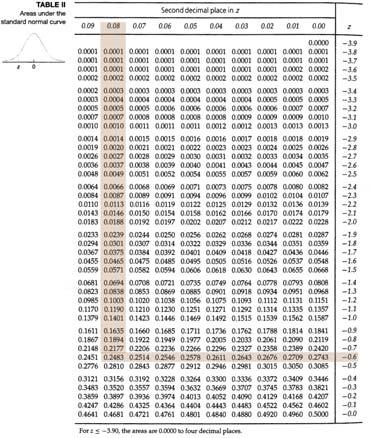

63 For z = 1.3 For z = 0.76 For z = 0.68 For z =
64 Examples with real data Intelligence quotients (IQs) are normally distributed with μ = 100 and σ = 16 What is the % of people who have IQs between 115 and 140? For x = 115, z = 115 μ/σ = /16 = 0.94 For x = 140, z = 140 μ/σ = /16 =.50 Area to left of 0.94 (from z table) = Area to left of.50 = So, = And, we can say that 16.74% of people have IQ between 115 and 140 We can also ask about a certain area, find a z score, then calculate a value (reversing the process we just covered) What is the IQ that is the cutoff for the top 10% for all people? In the z table, we see that is the value closest to 0.90 That corresponds to a z score =

65 z = 1.8 = x 100/16 Multiply both sides by SD = x = x 100 Add mean to both sides = x x = So, 90% of people have IQs below and 10% have higher IQs 65
66 Determine the area under the SNC that lies to the left of: Determine the area under the SNC that lies to the right of: Determine the area under the SNC that lies between:.18 and 1.44 and and 1.51 Find the z score for which the area under the SNC to its left is 0.05 or.5% Find the z score that has area of 0.70 to its right 66
67 Frequency and relative frequency distributions for heights of female college students (n = 3,64) at a small mid western college μ = 64.4 σ =.4 Ht (in) Freq Rel Freq What is the % of female students with heights between 65 and 70 inches? z = /.4 =.3 z 1 = /.4 = 0.5 Area to left of z = Area to left of z 1 = Area between = = or 39.1% of female students will have heights inches In the table, relative frequency between inches = = or 40.6% 67
68 68
69 69
70 Sample Distribution and Sampling Error We ve talked about how much time and money we can save by taking a sample from a large population instead of census But, a sample will guarantee a certain amount of sampling error (s and x will never be population mean and SD) If we are sampling from a normal population, we can expect that our sample will be normally distributed and x will be close to μ For a variable x and a given sample size, the distribution of the variable x is called the sampling distribution of the sample mean Example: Population is 5 starting players on a men s basketball team, players A, B, C, D, and E Player A B C D E Ht (in) µ = N x i = = If we take a random sample of players, we have the following sampling distribution of x with 10 possible combinations Sample Hts x A,B 76,78 77 A,C 76, A,D 76, A,E 76,86 81 B,C 78, B,D 78, B,E 78,86 8 C,D 79,81 80 C,E 79, D,E 81,
71 We see that mean height of players isn t likely to equal μ = 80.0, and only 1/10 sample means = 80 So, we can say that there is a 1/10 = 10% chance that x = μ Also, 3/10 samples have means within 1 inch of μ, so we can say that the probability is 0.3 or there is a 30% chance that a sample mean will be within 1 inch of μ Now, let s choose 4 players at random (only 5 possibilities): Sample A,B,C,D x A,B,C,E A,B,D,E 80.5 A,C,D,E B,C,D,E A graph for the distribution of sample means: Now, none of the sample means equal μ, but 4/5 or 80% are within 1 inch of μ or P(79.0 x 81.0) = 0.8 Graphs of sampling distributions as sample size increases n = n = n = 4 n =
72 This demonstrates that sampling error tends to be smaller for larger samples This is what we see with our basketball player example Sample size (n) # possible samples # within 1" of μ % within 1" of μ # within 0.5" of μ % within 0.5" of μ % 0 0% % 0% % 0% % 3 60% % 1 100% There is a simple relationship between the mean of variable and the population mean, μ µ = µ x x This means that if we take all possible x for any sample size and take the mean ( µ x, the population mean for the sample distribution), we will get μ, the entire population mean For our basketball example for sample size 4: µ x = = There is also a relationship between the standard deviation (s or SD) of the variable x with the population SD or σ σ = x σ n 7
73 For our basketball example for sample size 4: σ x = ( ) + ( ) + ( ) + ( ) + ( ) 5 σ x = = = Note: when sampling is done without replacement from a finite population (basketball example) the formula σ σ = x n will not give you exact sample SD, For all possible sample sizes: σ x Sample SD of size (n) x Example from U.S. Census Bureau Mean living space, μ, for a single family detached home is 1,74 sq. ft. and SD, σ, is 568 sq. ft. a) For sample of 5 single family homes, what is mean and SD of variable x? σ 568 µ x = µ = 1,74 σ = = = x n 5 b) For a sample size of 500? σ 568 µ x = µ = 1,74 σ = = = 5. 4 x n

74 Confidence Intervals for a Population Mean Remember, when we get a sample mean ( x ), we are getting an estimate of the population mean (μ) which we will call a point estimate A sample mean is usually not equal to the population mean because we will have sampling error Now, we will attach information to the estimate that will indicate the accuracy of that estimate, a confidence interval estimate for μ, or CI The more information we have for our sample (greater sample size) the more confident we will be that we are close to μ We should now know how to compute areas under the standard normal curve (SNC) between two critical values You should be able to do this whether you start with z scores or values of x From lecture 9: Computing a 95% CI is similar to finding the critical values that are the boundaries for the middle 95% of data for a population (as opposed to a sample) 74
?")
75 The difference is we are computing critical z values that are the boundaries for a CI surrounding our sample mean In other words, how confident are we that the population mean (μ) lies within the CI we have constructed around our sample mean ( x)? If we use calculations for a 95% CI then we are 95% confident that μ is within the CI An increase in sample size will lead to a more narrow CI surrounding x For a 95% CI, the critical z values will always be 1.96 to the left and 1.96 to the right = 0.05, and the area of 0.05 is divided by (for right and left side), so 0.05/ = In z table, the z value of 1.96 corresponds to the area under the SNC of The area of equal size to the right is always the same z value but positive 75

76 These critical values of z are given a special notation depending on our desired level of confidence (CL) We need to write the CL in the form of 1 α, where α is the number that must be subtracted from 1 to get the CL If we want a 95% CI, = 0.05 = α and the associated z value is z 0.05 But, because we want to split the area on the left and right side we want z α/ or z 0.05/ = z 0.05 This gives us the formula: α/ = (1 CL)/ For a CL of 90%: α/ = (1 0.90)/ = 0.05 So, we need critical cut off values of z 0.05 In the z table, the area under the SNC of 0.05 corresponds to a z value of 1.64 In most cases, we are interested in CL s of 90%, 95%, and 99% (z = 1.64, 1.96, and.57, respectively) 76
77 Confidence Intervals with known σ If we know the population standard deviation (σ), the following formulas will give us the CI surrounding x x z α / σ n lower limit and σ x + zα / n upper limit or x ± z α / σ n Example: Take a sample of verbal SAT scores from n = 40 high school students. We know the population SD is σ = 83.8 and our sample mean is x = Construct a 95% CI First we need critical values for z α/ and z α/ α = (1 CL) = (1 0.95) = 0.05 z 0.05 = 1.96 For our 95% CI: x z α x + z σ 83.8 / = = = = 44.5 n 40 α σ 83.8 / = = = = n 40 77
78 This is interpreted as, we are 95% confident that the population mean (μ) lies within the range of This also implies that there is a 5% chance that μ does not fall into this interval Actually, μ = from a population of 78 students Graphically, the 95% CI would appear like this: x µ
.")
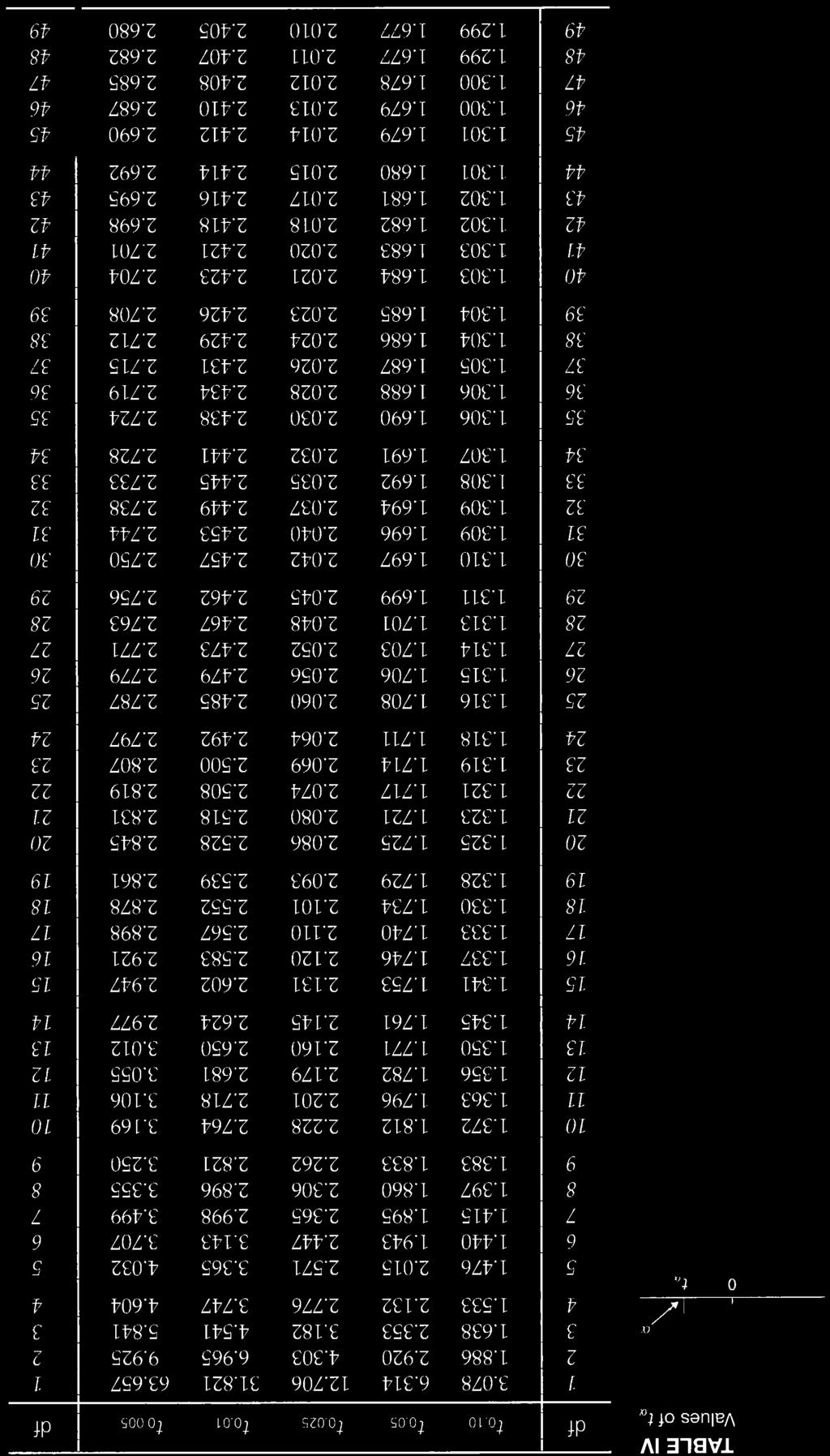
 of the table represent an estimation of z scores but for smaller samples To get values of t, we need things: α and")
79 Confidence Intervals with unknown σ This is very similar to CI with known σ, but there are things we must do differently 1. First, we have to estimate σ using our sample data to calculate a sample SD (s). Next, we can t use the z table (that s only for large populations), so we use a t table (for small populations) The numbers in the body (middle) of the table represent an estimation of z scores but for smaller samples To get values of t, we need things: α and degrees of freedom (df) which is n 1 (n = sample size) 79
/ The equations to calculate CI s are identical to solve but we use a t instead of z value and sample SD (s) instead of σ x + tα / s n x tα / s n We")
80 In the example above, n = 14 so df = 13, and if we re looking for the critical value of t α, we look for t 0.05 across the top of the table and df along the side to get We find α/ with the same equation: α/ = (1 CL)/ The equations to calculate CI s are identical to solve but we use a t instead of z value and sample SD (s) instead of σ x + tα / s n x tα / s n We will use the same data set for verbal SAT scores for an example (sample of 40 scores) From beginning of semester, we used these formulas to calculate s ( x ) i x s = s = s n 1 80

81 The sample SD from this sample data set is s = 96.9 and sample mean is the same, x= The t value for a 95% CI is t 0.05 (remember α/) with df = 39 so critical t 0.05 =.03 We put these values into the new equations: x t α s 96.9 / = n = x + t s = n α / =
82 This is has the same interpretation, we are 95% confident that the population mean (μ) lies within the range of But, notice the 95% CI is wider using a sample SD Remember, μ = from a population of 78 students Graphically, let s compare the 95% CI with and without knowing σ: With σ With s
83 83
84 Hypothesis Testing One of the primary uses of calculated statistics is to make decisions about the value of a parameter (inferential stats) Examples: Is the mean weight, μ, of bags of pretzels produced by a company really 454 grams as advertised? Has the mean age of all cars in use increased from the 1995 mean of 8.5 years? Has the mean weight of white tail deer does in a particular area of Mississippi increased or decreased from year to year? We can attempt to answer these questions by setting up a null hypothesis, H 0, to test If we have a null hypothesis, we need at least one alternative hypothesis, H 1 or H a, to test against For the pretzel example: H 0 : mean wt. of bags is 454 g; H 0 : μ = 454 g H a : mean wt. of bags is not 454 g; H a : μ 454 g We call this a two tailed test because H a can be > or < There are also one tailed tests where H a is either > or < 84
 For a hypothesis test, we call the associated α value the significance level Example: If we want to be 95% confident that our")
85 We will concentrate on two tailed tests We reject our H 0 if our calculated z value falls out of the do not reject region of the standard normal curve (SNC) Notice that the two tailed SNC above is identical to the CI curve we discussed in Lectures 9 and 10 (below) For a hypothesis test, we call the associated α value the significance level Example: If we want to be 95% confident that our sample mean, x, is or is not equal to our hypothesis mean, μ, we use a significance level of α = 0.05 Recall from Lecture 9, the associated critical z value for α = 0.05 with two tails (so α/) is ±
Elementary Statistics
 Elementary Statistics Q: What is data? Q: What does the data look like? Q: What conclusions can we draw from the data? Q: Where is the middle of the data? Q: Why is the spread of the data important? Q:
MATH 1150 Chapter 2 Notation and Terminology
 MATH 1150 Chapter 2 Notation and Terminology Categorical Data The following is a dataset for 30 randomly selected adults in the U.S., showing the values of two categorical variables: whether or not the
Chapter 2: Tools for Exploring Univariate Data
 Stats 11 (Fall 2004) Lecture Note Introduction to Statistical Methods for Business and Economics Instructor: Hongquan Xu Chapter 2: Tools for Exploring Univariate Data Section 2.1: Introduction What is
Stat 101 Exam 1 Important Formulas and Concepts 1
 1 Chapter 1 1.1 Definitions Stat 101 Exam 1 Important Formulas and Concepts 1 1. Data Any collection of numbers, characters, images, or other items that provide information about something. 2. Categorical/Qualitative
TOPIC: Descriptive Statistics Single Variable
 TOPIC: Descriptive Statistics Single Variable I. Numerical data summary measurements A. Measures of Location. Measures of central tendency Mean; Median; Mode. Quantiles - measures of noncentral tendency
Business Statistics. Lecture 10: Course Review
 Business Statistics Lecture 10: Course Review 1 Descriptive Statistics for Continuous Data Numerical Summaries Location: mean, median Spread or variability: variance, standard deviation, range, percentiles,
STT 315 This lecture is based on Chapter 2 of the textbook.
 STT 315 This lecture is based on Chapter 2 of the textbook. Acknowledgement: Author is thankful to Dr. Ashok Sinha, Dr. Jennifer Kaplan and Dr. Parthanil Roy for allowing him to use/edit some of their
STATISTICS 1 REVISION NOTES
 STATISTICS 1 REVISION NOTES Statistical Model Representing and summarising Sample Data Key words: Quantitative Data This is data in NUMERICAL FORM such as shoe size, height etc. Qualitative Data This is
CIVL 7012/8012. Collection and Analysis of Information
 CIVL 7012/8012 Collection and Analysis of Information Uncertainty in Engineering Statistics deals with the collection and analysis of data to solve real-world problems. Uncertainty is inherent in all real
Descriptive Statistics-I. Dr Mahmoud Alhussami
 Descriptive Statistics-I Dr Mahmoud Alhussami Biostatistics What is the biostatistics? A branch of applied math. that deals with collecting, organizing and interpreting data using well-defined procedures.
F78SC2 Notes 2 RJRC. If the interest rate is 5%, we substitute x = 0.05 in the formula. This gives
 F78SC2 Notes 2 RJRC Algebra It is useful to use letters to represent numbers. We can use the rules of arithmetic to manipulate the formula and just substitute in the numbers at the end. Example: 100 invested
Sampling, Frequency Distributions, and Graphs (12.1)
") 1 Sampling, Frequency Distributions, and Graphs (1.1) Design: Plan how to obtain the data. What are typical Statistical Methods? Collect the data, which is then subjected to statistical analysis, which
1 Sampling, Frequency Distributions, and Graphs (1.1) Design: Plan how to obtain the data. What are typical Statistical Methods? Collect the data, which is then subjected to statistical analysis, which
What is statistics? Statistics is the science of: Collecting information. Organizing and summarizing the information collected
 What is statistics? Statistics is the science of: Collecting information Organizing and summarizing the information collected Analyzing the information collected in order to draw conclusions Two types
Nicole Dalzell. July 2, 2014
 UNIT 1: INTRODUCTION TO DATA LECTURE 3: EDA (CONT.) AND INTRODUCTION TO STATISTICAL INFERENCE VIA SIMULATION STATISTICS 101 Nicole Dalzell July 2, 2014 Teams and Announcements Team1 = Houdan Sai Cui Huanqi
Business Statistics. Lecture 9: Simple Regression
 Business Statistics Lecture 9: Simple Regression 1 On to Model Building! Up to now, class was about descriptive and inferential statistics Numerical and graphical summaries of data Confidence intervals
STP 420 INTRODUCTION TO APPLIED STATISTICS NOTES
 INTRODUCTION TO APPLIED STATISTICS NOTES PART - DATA CHAPTER LOOKING AT DATA - DISTRIBUTIONS Individuals objects described by a set of data (people, animals, things) - all the data for one individual make
MIDTERM EXAMINATION (Spring 2011) STA301- Statistics and Probability
 STA301- Statistics and Probability") STA301- Statistics and Probability Solved MCQS From Midterm Papers March 19,2012 MC100401285 Moaaz.pk@gmail.com Mc100401285@gmail.com PSMD01 MIDTERM EXAMINATION (Spring 2011) STA301- Statistics and Probability
STA301- Statistics and Probability Solved MCQS From Midterm Papers March 19,2012 MC100401285 Moaaz.pk@gmail.com Mc100401285@gmail.com PSMD01 MIDTERM EXAMINATION (Spring 2011) STA301- Statistics and Probability
Marketing Research Session 10 Hypothesis Testing with Simple Random samples (Chapter 12)
") Marketing Research Session 10 Hypothesis Testing with Simple Random samples (Chapter 12) Remember: Z.05 = 1.645, Z.01 = 2.33 We will only cover one-sided hypothesis testing (cases 12.3, 12.4.2, 12.5.2,
Marketing Research Session 10 Hypothesis Testing with Simple Random samples (Chapter 12) Remember: Z.05 = 1.645, Z.01 = 2.33 We will only cover one-sided hypothesis testing (cases 12.3, 12.4.2, 12.5.2,
Marquette University MATH 1700 Class 5 Copyright 2017 by D.B. Rowe
 Class 5 Daniel B. Rowe, Ph.D. Department of Mathematics, Statistics, and Computer Science Copyright 2017 by D.B. Rowe 1 Agenda: Recap Chapter 3.2-3.3 Lecture Chapter 4.1-4.2 Review Chapter 1 3.1 (Exam
(quantitative or categorical variables) Numerical descriptions of center, variability, position (quantitative variables)
 Numerical descriptions of center, variability, position (quantitative variables)") 3. Descriptive Statistics Describing data with tables and graphs (quantitative or categorical variables) Numerical descriptions of center, variability, position (quantitative variables) Bivariate descriptions
3. Descriptive Statistics Describing data with tables and graphs (quantitative or categorical variables) Numerical descriptions of center, variability, position (quantitative variables) Bivariate descriptions
Section 3.2 Measures of Central Tendency
 Section 3.2 Measures of Central Tendency 1 of 149 Section 3.2 Objectives Determine the mean, median, and mode of a population and of a sample Determine the weighted mean of a data set and the mean of a
Why should you care?? Intellectual curiosity. Gambling. Mathematically the same as the ESP decision problem we discussed in Week 4.
 I. Probability basics (Sections 4.1 and 4.2) Flip a fair (probability of HEADS is 1/2) coin ten times. What is the probability of getting exactly 5 HEADS? What is the probability of getting exactly 10
Lecture Slides. Elementary Statistics Twelfth Edition. by Mario F. Triola. and the Triola Statistics Series. Section 3.1- #
 Lecture Slides Elementary Statistics Twelfth Edition and the Triola Statistics Series by Mario F. Triola Chapter 3 Statistics for Describing, Exploring, and Comparing Data 3-1 Review and Preview 3-2 Measures
Math 223 Lecture Notes 3/15/04 From The Basic Practice of Statistics, bymoore
 Math 223 Lecture Notes 3/15/04 From The Basic Practice of Statistics, bymoore Chapter 3 continued Describing distributions with numbers Measuring spread of data: Quartiles Definition 1: The interquartile
Lecture 1: Description of Data. Readings: Sections 1.2,
 Lecture 1: Description of Data Readings: Sections 1.,.1-.3 1 Variable Example 1 a. Write two complete and grammatically correct sentences, explaining your primary reason for taking this course and then
Objective A: Mean, Median and Mode Three measures of central of tendency: the mean, the median, and the mode.
 Chapter 3 Numerically Summarizing Data Chapter 3.1 Measures of Central Tendency Objective A: Mean, Median and Mode Three measures of central of tendency: the mean, the median, and the mode. A1. Mean The
Introduction to Statistics
 Introduction to Statistics Data and Statistics Data consists of information coming from observations, counts, measurements, or responses. Statistics is the science of collecting, organizing, analyzing,
Section 3: Simple Linear Regression
 Section 3: Simple Linear Regression Carlos M. Carvalho The University of Texas at Austin McCombs School of Business http://faculty.mccombs.utexas.edu/carlos.carvalho/teaching/ 1 Regression: General Introduction
Quantitative Methods for Decision Making
 January 14, 2012 Lecture 3 Probability Theory Definition Mutually exclusive events: Two events A and B are mutually exclusive if A B = φ Definition Special Addition Rule: Let A and B be two mutually exclusive
AP Statistics Cumulative AP Exam Study Guide
 AP Statistics Cumulative AP Eam Study Guide Chapters & 3 - Graphs Statistics the science of collecting, analyzing, and drawing conclusions from data. Descriptive methods of organizing and summarizing statistics
Review of Statistics
 Review of Statistics Topics Descriptive Statistics Mean, Variance Probability Union event, joint event Random Variables Discrete and Continuous Distributions, Moments Two Random Variables Covariance and
Review of Statistics 101
 Review of Statistics 101 We review some important themes from the course 1. Introduction Statistics- Set of methods for collecting/analyzing data (the art and science of learning from data). Provides methods
1-1. Chapter 1. Sampling and Descriptive Statistics by The McGraw-Hill Companies, Inc. All rights reserved.
 1-1 Chapter 1 Sampling and Descriptive Statistics 1-2 Why Statistics? Deal with uncertainty in repeated scientific measurements Draw conclusions from data Design valid experiments and draw reliable conclusions
Math 2000 Practice Final Exam: Homework problems to review. Problem numbers
 Math 2000 Practice Final Exam: Homework problems to review Pages: Problem numbers 52 20 65 1 181 14 189 23, 30 245 56 256 13 280 4, 15 301 21 315 18 379 14 388 13 441 13 450 10 461 1 553 13, 16 561 13,
Chapter 4. Displaying and Summarizing. Quantitative Data
 STAT 141 Introduction to Statistics Chapter 4 Displaying and Summarizing Quantitative Data Bin Zou (bzou@ualberta.ca) STAT 141 University of Alberta Winter 2015 1 / 31 4.1 Histograms 1 We divide the range
Psych 230. Psychological Measurement and Statistics
 Psych 230 Psychological Measurement and Statistics Pedro Wolf December 9, 2009 This Time. Non-Parametric statistics Chi-Square test One-way Two-way Statistical Testing 1. Decide which test to use 2. State
6 THE NORMAL DISTRIBUTION
 CHAPTER 6 THE NORMAL DISTRIBUTION 341 6 THE NORMAL DISTRIBUTION Figure 6.1 If you ask enough people about their shoe size, you will find that your graphed data is shaped like a bell curve and can be described
Business Statistics. Lecture 10: Correlation and Linear Regression
 Business Statistics Lecture 10: Correlation and Linear Regression Scatterplot A scatterplot shows the relationship between two quantitative variables measured on the same individuals. It displays the Form
Lecture 26: Chapter 10, Section 2 Inference for Quantitative Variable Confidence Interval with t
 Lecture 26: Chapter 10, Section 2 Inference for Quantitative Variable Confidence Interval with t t Confidence Interval for Population Mean Comparing z and t Confidence Intervals When neither z nor t Applies
Identify the scale of measurement most appropriate for each of the following variables. (Use A = nominal, B = ordinal, C = interval, D = ratio.
 Answers to Items from Problem Set 1 Item 1 Identify the scale of measurement most appropriate for each of the following variables. (Use A = nominal, B = ordinal, C = interval, D = ratio.) a. response latency
Slide 1. Slide 2. Slide 3. Pick a Brick. Daphne. 400 pts 200 pts 300 pts 500 pts 100 pts. 300 pts. 300 pts 400 pts 100 pts 400 pts.
 Slide 1 Slide 2 Daphne Phillip Kathy Slide 3 Pick a Brick 100 pts 200 pts 500 pts 300 pts 400 pts 200 pts 300 pts 500 pts 100 pts 300 pts 400 pts 100 pts 400 pts 100 pts 200 pts 500 pts 100 pts 400 pts
Chapter 16. Simple Linear Regression and dcorrelation
 Chapter 16 Simple Linear Regression and dcorrelation 16.1 Regression Analysis Our problem objective is to analyze the relationship between interval variables; regression analysis is the first tool we will
Units. Exploratory Data Analysis. Variables. Student Data
 Units Exploratory Data Analysis Bret Larget Departments of Botany and of Statistics University of Wisconsin Madison Statistics 371 13th September 2005 A unit is an object that can be measured, such as
AP Final Review II Exploring Data (20% 30%)
") AP Final Review II Exploring Data (20% 30%) Quantitative vs Categorical Variables Quantitative variables are numerical values for which arithmetic operations such as means make sense. It is usually a measure
AP Final Review II Exploring Data (20% 30%) Quantitative vs Categorical Variables Quantitative variables are numerical values for which arithmetic operations such as means make sense. It is usually a measure
Lecture 2 and Lecture 3
 Lecture 2 and Lecture 3 1 Lecture 2 and Lecture 3 We can describe distributions using 3 characteristics: shape, center and spread. These characteristics have been discussed since the foundation of statistics.
Introduction to bivariate analysis
 Introduction to bivariate analysis When one measurement is made on each observation, univariate analysis is applied. If more than one measurement is made on each observation, multivariate analysis is applied.
Determining the Spread of a Distribution
 Determining the Spread of a Distribution 1.3-1.5 Cathy Poliak, Ph.D. cathy@math.uh.edu Department of Mathematics University of Houston Lecture 3-2311 Lecture 3-2311 1 / 58 Outline 1 Describing Quantitative
Determining the Spread of a Distribution
 Determining the Spread of a Distribution 1.3-1.5 Cathy Poliak, Ph.D. cathy@math.uh.edu Department of Mathematics University of Houston Lecture 3-2311 Lecture 3-2311 1 / 58 Outline 1 Describing Quantitative
Lecture 18: Simple Linear Regression
 Lecture 18: Simple Linear Regression BIOS 553 Department of Biostatistics University of Michigan Fall 2004 The Correlation Coefficient: r The correlation coefficient (r) is a number that measures the strength
Introduction to bivariate analysis
 Introduction to bivariate analysis When one measurement is made on each observation, univariate analysis is applied. If more than one measurement is made on each observation, multivariate analysis is applied.
Final Exam STAT On a Pareto chart, the frequency should be represented on the A) X-axis B) regression C) Y-axis D) none of the above
 X-axis B) regression C) Y-axis D) none of the above") King Abdul Aziz University Faculty of Sciences Statistics Department Final Exam STAT 0 First Term 49-430 A 40 Name No ID: Section: You have 40 questions in 9 pages. You have 90 minutes to solve the exam.
King Abdul Aziz University Faculty of Sciences Statistics Department Final Exam STAT 0 First Term 49-430 A 40 Name No ID: Section: You have 40 questions in 9 pages. You have 90 minutes to solve the exam.
Marquette University Executive MBA Program Statistics Review Class Notes Summer 2018
 Marquette University Executive MBA Program Statistics Review Class Notes Summer 2018 Chapter One: Data and Statistics Statistics A collection of procedures and principles
Multiple Regression Analysis
 Multiple Regression Analysis y = β 0 + β 1 x 1 + β 2 x 2 +... β k x k + u 2. Inference 0 Assumptions of the Classical Linear Model (CLM)! So far, we know: 1. The mean and variance of the OLS estimators
Probability Distributions
 CONDENSED LESSON 13.1 Probability Distributions In this lesson, you Sketch the graph of the probability distribution for a continuous random variable Find probabilities by finding or approximating areas
LC OL - Statistics. Types of Data
 LC OL - Statistics Types of Data Question 1 Characterise each of the following variables as numerical or categorical. In each case, list any three possible values for the variable. (i) Eye colours in a
Unit 4 Probability. Dr Mahmoud Alhussami
 Unit 4 Probability Dr Mahmoud Alhussami Probability Probability theory developed from the study of games of chance like dice and cards. A process like flipping a coin, rolling a die or drawing a card from
Topic 3: Introduction to Statistics. Algebra 1. Collecting Data. Table of Contents. Categorical or Quantitative? What is the Study of Statistics?!
 Topic 3: Introduction to Statistics Collecting Data We collect data through observation, surveys and experiments. We can collect two different types of data: Categorical Quantitative Algebra 1 Table of
Chapter 01 : What is Statistics?
 Chapter 01 : What is Statistics? Feras Awad Data: The information coming from observations, counts, measurements, and responses. Statistics: The science of collecting, organizing, analyzing, and interpreting
Sem. 1 Review Ch. 1-3
 AP Stats Sem. 1 Review Ch. 1-3 Name 1. You measure the age, marital status and earned income of an SRS of 1463 women. The number and type of variables you have measured is a. 1463; all quantitative. b.
CHAPTER 7 THE SAMPLING DISTRIBUTION OF THE MEAN. 7.1 Sampling Error; The need for Sampling Distributions
 CHAPTER 7 THE SAMPLING DISTRIBUTION OF THE MEAN 7.1 Sampling Error; The need for Sampling Distributions Sampling Error the error resulting from using a sample characteristic (statistic) to estimate a population
Vocabulary: Samples and Populations
 Vocabulary: Samples and Populations Concept Different types of data Categorical data results when the question asked in a survey or sample can be answered with a nonnumerical answer. For example if we
Histograms allow a visual interpretation
 Chapter 4: Displaying and Summarizing i Quantitative Data s allow a visual interpretation of quantitative (numerical) data by indicating the number of data points that lie within a range of values, called
appstats8.notebook October 11, 2016
 Chapter 8 Linear Regression Objective: Students will construct and analyze a linear model for a given set of data. Fat Versus Protein: An Example pg 168 The following is a scatterplot of total fat versus
Unit 2. Describing Data: Numerical
 Unit 2 Describing Data: Numerical Describing Data Numerically Describing Data Numerically Central Tendency Arithmetic Mean Median Mode Variation Range Interquartile Range Variance Standard Deviation Coefficient
Math 120 Introduction to Statistics Mr. Toner s Lecture Notes 3.1 Measures of Central Tendency
 Math 1 Introduction to Statistics Mr. Toner s Lecture Notes 3.1 Measures of Central Tendency The word average: is very ambiguous and can actually refer to the mean, median, mode or midrange. Notation:
Statistical Inference for Means
 Statistical Inference for Means Jamie Monogan University of Georgia February 18, 2011 Jamie Monogan (UGA) Statistical Inference for Means February 18, 2011 1 / 19 Objectives By the end of this meeting,
STAT 200 Chapter 1 Looking at Data - Distributions
 STAT 200 Chapter 1 Looking at Data - Distributions What is Statistics? Statistics is a science that involves the design of studies, data collection, summarizing and analyzing the data, interpreting the
STAT/SOC/CSSS 221 Statistical Concepts and Methods for the Social Sciences. Random Variables
 STAT/SOC/CSSS 221 Statistical Concepts and Methods for the Social Sciences Random Variables Christopher Adolph Department of Political Science and Center for Statistics and the Social Sciences University
Stat 20 Midterm 1 Review
 Stat 20 Midterm Review February 7, 2007 This handout is intended to be a comprehensive study guide for the first Stat 20 midterm exam. I have tried to cover all the course material in a way that targets
Math 221, REVIEW, Instructor: Susan Sun Nunamaker
 Math 221, REVIEW, Instructor: Susan Sun Nunamaker Good Luck & Contact me through through e-mail if you have any questions. 1. Bar graphs can only be vertical. a. true b. false 2.
The empirical ( ) rule
 rule") The empirical (68-95-99.7) rule With a bell shaped distribution, about 68% of the data fall within a distance of 1 standard deviation from the mean. 95% fall within 2 standard deviations of the mean. 99.7%
The empirical (68-95-99.7) rule With a bell shaped distribution, about 68% of the data fall within a distance of 1 standard deviation from the mean. 95% fall within 2 standard deviations of the mean. 99.7%
Dover- Sherborn High School Mathematics Curriculum Probability and Statistics
 Mathematics Curriculum A. DESCRIPTION This is a full year courses designed to introduce students to the basic elements of statistics and probability. Emphasis is placed on understanding terminology and
CS 361: Probability & Statistics
 January 24, 2018 CS 361: Probability & Statistics Relationships in data Standard coordinates If we have two quantities of interest in a dataset, we might like to plot their histograms and compare the two
Announcements. Lecture 1 - Data and Data Summaries. Data. Numerical Data. all variables. continuous discrete. Homework 1 - Out 1/15, due 1/22
 Announcements Announcements Lecture 1 - Data and Data Summaries Statistics 102 Colin Rundel January 13, 2013 Homework 1 - Out 1/15, due 1/22 Lab 1 - Tomorrow RStudio accounts created this evening Try logging
Final Exam - Solutions
 Ecn 102 - Analysis of Economic Data University of California - Davis March 19, 2010 Instructor: John Parman Final Exam - Solutions You have until 5:30pm to complete this exam. Please remember to put your
Chapter 6. The Standard Deviation as a Ruler and the Normal Model 1 /67
 Chapter 6 The Standard Deviation as a Ruler and the Normal Model 1 /67 Homework Read Chpt 6 Complete Reading Notes Do P129 1, 3, 5, 7, 15, 17, 23, 27, 29, 31, 37, 39, 43 2 /67 Objective Students calculate
QUANTITATIVE DATA. UNIVARIATE DATA data for one variable
 QUANTITATIVE DATA Recall that quantitative (numeric) data values are numbers where data take numerical values for which it is sensible to find averages, such as height, hourly pay, and pulse rates. UNIVARIATE
Lecture 11. Data Description Estimation
 Lecture 11 Data Description Estimation Measures of Central Tendency (continued, see last lecture) Sample mean, population mean Sample mean for frequency distributions The median The mode The midrange 3-22
CHAPTER 5: EXPLORING DATA DISTRIBUTIONS. Individuals are the objects described by a set of data. These individuals may be people, animals or things.
 (c) Epstein 2013 Chapter 5: Exploring Data Distributions Page 1 CHAPTER 5: EXPLORING DATA DISTRIBUTIONS 5.1 Creating Histograms Individuals are the objects described by a set of data. These individuals
AP Statistics Bivariate Data Analysis Test Review. Multiple-Choice
 Name Period AP Statistics Bivariate Data Analysis Test Review Multiple-Choice 1. The correlation coefficient measures: (a) Whether there is a relationship between two variables (b) The strength of the
Lecture Notes 2: Variables and graphics
 Highlights: Lecture Notes 2: Variables and graphics Quantitative vs. qualitative variables Continuous vs. discrete and ordinal vs. nominal variables Frequency distributions Pie charts Bar charts Histograms
Introduction to Probability and Statistics Slides 1 Chapter 1
 1 Introduction to Probability and Statistics Slides 1 Chapter 1 Prof. Ammar M. Sarhan, asarhan@mathstat.dal.ca Department of Mathematics and Statistics, Dalhousie University Fall Semester 2010 Course outline
Chapter 16. Simple Linear Regression and Correlation
 Chapter 16 Simple Linear Regression and Correlation 16.1 Regression Analysis Our problem objective is to analyze the relationship between interval variables; regression analysis is the first tool we will
IAM 530 ELEMENTS OF PROBABILITY AND STATISTICS LECTURE 3-RANDOM VARIABLES
 IAM 530 ELEMENTS OF PROBABILITY AND STATISTICS LECTURE 3-RANDOM VARIABLES VARIABLE Studying the behavior of random variables, and more importantly functions of random variables is essential for both the
20 Hypothesis Testing, Part I
 20 Hypothesis Testing, Part I Bob has told Alice that the average hourly rate for a lawyer in Virginia is $200 with a standard deviation of $50, but Alice wants to test this claim. If Bob is right, she
THE SAMPLING DISTRIBUTION OF THE MEAN
 THE SAMPLING DISTRIBUTION OF THE MEAN COGS 14B JANUARY 26, 2017 TODAY Sampling Distributions Sampling Distribution of the Mean Central Limit Theorem INFERENTIAL STATISTICS Inferential statistics: allows
STA 218: Statistics for Management
 Al Nosedal. University of Toronto. Fall 2017 My momma always said: Life was like a box of chocolates. You never know what you re gonna get. Forrest Gump. Problem How much do people with a bachelor s degree
Unit Two Descriptive Biostatistics. Dr Mahmoud Alhussami
 Unit Two Descriptive Biostatistics Dr Mahmoud Alhussami Descriptive Biostatistics The best way to work with data is to summarize and organize them. Numbers that have not been summarized and organized are
Describing Distributions with Numbers
 Describing Distributions with Numbers Using graphs, we could determine the center, spread, and shape of the distribution of a quantitative variable. We can also use numbers (called summary statistics)
Section 7.1 Properties of the Normal Distribution
 Section 7.1 Properties of the Normal Distribution In Chapter 6, talked about probability distributions. Coin flip problem: Difference of two spinners: The random variable x can only take on certain discrete
Steve Smith Tuition: Maths Notes
 Maths Notes : Discrete Random Variables Version. Steve Smith Tuition: Maths Notes e iπ + = 0 a + b = c z n+ = z n + c V E + F = Discrete Random Variables Contents Intro The Distribution of Probabilities
Preliminary Statistics course. Lecture 1: Descriptive Statistics
 Preliminary Statistics course Lecture 1: Descriptive Statistics Rory Macqueen (rm43@soas.ac.uk), September 2015 Organisational Sessions: 16-21 Sep. 10.00-13.00, V111 22-23 Sep. 15.00-18.00, V111 24 Sep.
Table of z values and probabilities for the standard normal distribution. z is the first column plus the top row. Each cell shows P(X z).
.") Table of z values and probabilities for the standard normal distribution. z is the first column plus the top row. Each cell shows P(X z). For example P(X.04) =.8508. For z < 0 subtract the value from,
Table of z values and probabilities for the standard normal distribution. z is the first column plus the top row. Each cell shows P(X z). For example P(X.04) =.8508. For z < 0 subtract the value from,
Vehicle Freq Rel. Freq Frequency distribution. Statistics
 1.1 STATISTICS Statistics is the science of data. This involves collecting, summarizing, organizing, and analyzing data in order to draw meaningful conclusions about the universe from which the data is
Describing distributions with numbers
 Describing distributions with numbers A large number or numerical methods are available for describing quantitative data sets. Most of these methods measure one of two data characteristics: The central
M 225 Test 1 B Name SHOW YOUR WORK FOR FULL CREDIT! Problem Max. Points Your Points Total 75
 M 225 Test 1 B Name SHOW YOUR WORK FOR FULL CREDIT! Problem Max. Points Your Points 1-13 13 14 3 15 8 16 4 17 10 18 9 19 7 20 3 21 16 22 2 Total 75 1 Multiple choice questions (1 point each) 1. Look at
Statistics for Managers using Microsoft Excel 6 th Edition
 Statistics for Managers using Microsoft Excel 6 th Edition Chapter 3 Numerical Descriptive Measures 3-1 Learning Objectives In this chapter, you learn: To describe the properties of central tendency, variation,
Keller: Stats for Mgmt & Econ, 7th Ed July 17, 2006
 Chapter 17 Simple Linear Regression and Correlation 17.1 Regression Analysis Our problem objective is to analyze the relationship between interval variables; regression analysis is the first tool we will
Statistics 100 Exam 2 March 8, 2017
 STAT 100 EXAM 2 Spring 2017 (This page is worth 1 point. Graded on writing your name and net id clearly and circling section.) PRINT NAME (Last name) (First name) net ID CIRCLE SECTION please! L1 (MWF
What is Statistics? Statistics is the science of understanding data and of making decisions in the face of variability and uncertainty.
 What is Statistics? Statistics is the science of understanding data and of making decisions in the face of variability and uncertainty. Statistics is a field of study concerned with the data collection,