What is statistics? Statistics is the science of: Collecting information. Organizing and summarizing the information collected

Transcription

1 What is statistics? Statistics is the science of: Collecting information Organizing and summarizing the information collected Analyzing the information collected in order to draw conclusions

2 Two types of Statistics Descriptive Statistics Organizing and summarizing the information collected. Inferential Statistics Draws conclusion from the information collected.

3 Chapter 1 Exploring Data

4 Lesson 1-1, Displaying Distributions with Graphs Bar Graphs and Pie Charts

5 Data Individuals are objects described by a set of data. Individuals may be people, animals or things. Variable is any characteristic of an individual. A variable can take different values for different individuals

6 Types of Variables Categorical variable allows for classification of individuals based on some attribute or characteristics. Quantitative variable provides numerical measures of individuals.

7 Example, Page 7, #1.2 Data from a medical study contain values of many variables for each of the people who where subjects of the study. Which of the following variables are categorical and which are quantitative?

8 Example, Page 7, #1.2 a) Gender (female or male) categorical b) Age (years) Quantitative c) Race (Asian, black, white or other) categorical d. Smoker (yes or no) categorical e) Systolic blood pressure (millimeters of mercury) Quantitative f) Level of calcium in blood (micrograms per milliliter) Quantitative

9 Distribution Distribution Tells us what values the variable takes and how often it takes each value

10 Displaying Distributions Categorical Variables Bar Graphs Pie Charts Quantitative Variables Dotplots Stemplots Histograms

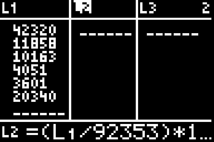
11 Example Page 11, #1.6 In 1997 there were 92,353 deaths from accidents in the United States. Among these were deaths from Motor vehicle accidents, 11,858 from falls, 10,163 from poisoning, 4051 from drowning, and 3601 from fires. A) Find the percent of accidental deaths from each of these causes, rounded to the nearest percent. What percent of accidental deaths were due to other causes?

12 Example Page 11, #1.6 Accidents Number Percentage Motor Vehicle 42,340 42, % Falls 11,858 Poisoning 10,163 Drowning 4051 Fires 3601 Other Causes 20,340 Total 92,353 92,353 13% 11% 4% 4% 22% 100%

13 Example Page 11, #1.6 STAT

14 Example Page 11, #1.6

15 Example Page 11, #1.6 B) Make a well-labeled bar graph of the distribution of causes of accidental deaths. Be sure to include an other causes bar.

16 Percentage of Accidental Deaths Example Page 11, #1.6 US Accidental Death MV Falls Poison Drown Fires OC Causes of Accidental Deaths

17 Example Page 11, #1.6 C) Would it also be correct to use a pie chart to display these data? If so, construct the pie chart. If not explain why not. Yes, since categories represent parts of a whole.

18 Example Page 11, #1.6 Accidents Number Percentage MV 42,340 46% Falls 11,858 13% Poisoning 10,163 11% Drowning % Fires % OC 20,340 22% Total 92, % Pie Chart

19 Example Page 11, #1.6

20 Example Page 11, #1.6 US Accidental Deaths % Motor Vehicle Falls 4% 4% 11% 13% 46% Poisoning Drowning Fires Other Causes

21 Lesson 1-1, Displaying Distributions with Graphs Dot Plots and Stem Leaf Plots

22 Overall Pattern of Distribution (Quantitative Variables) Center Divides the data in half Spread Smallest to largest values Shape Skewness of the data Outlier Data that falls outside of the pattern

23 Example Page 16, #1.8 Are you driving a gas guzzler? Table 1.3 displays the highway gas mileage for 32 model year 2000 midsize cars. A). Make a dot plot of these data.

24 Example Page 16, #1.8

25 Example Page 16, # Highway Gas Mileage

26 Example Page 16, #1.8 B) Describe the shape, center, and spread of the distribution of gas mileages. Are there any potential outliers? The shape of the distribution is skewed to the left, with a major peak at 28 and a minor peak at 24. The spread is relatively narrow (21 to 32 mpg). The two observations at 21 and the observation at 32 appear to outliers. The center is 28 mpg.

27 Example Page 35, #1.28 In 1978 the English scientist Henry Cavendish measured the density of the earth by careful work with a torsion balance. The variable recorded was the density of the earth as a multiple of the density water. Here are Cavendish s 29 measurements:

28 Example Page 35, # Present these measurements graphically in a stemplot. Discuss the shape, center, and spread of the distribution. Are there any outliers? What is estimate of the density of the earth based on these measurements?

29 Example Page 35, #1.28 Density of the Earth = 4.88% The shape of the distribution is roughly symmetric with one possible outlier at 4.88 that is somewhat low. The spread between 4.88 to The center of the distribution if between 5.4 and 5.5. Based on the plot, we would estimate the Earth s density to be about halfway between 5.4 and 5.5.

30 Lesson 1-1 Displaying Distributions with Graphs Histograms and Relative Frequency Graphs

31 Frequency (Count) Histogram and categories Age of Spring 1998 Stat 250 Students GPAs of Spring 1998 Stat 250 Students n=92 students Age (in years) n=92 students GPA too few categories too many categories

32 Example Histogram Suppose you are considering investing in a Roth IRA. You collect the data table, which represent the three-year rate of return (in percent) for 40 small capitalization growth mutual funds

33 Example Histogram STAT

34 Example Histogram A) Construct a histogram to display these data. Record your class intervals and counts Step 1 Find the class intervals Locate the smallest number (10.8) and the largest number (47.7) Lower class limit will be 10.0 with a class width of 5

35 Example Histogram 3-yr Rate of Return Total Frequency

36 Example Histogram Step 2 Graph it using the TI Stat Plot 2 nd Y= Window

37 Example Histogram Graph Trace

38 Frequency Example - Histogram 12 3 Year Rate of Return of Mutual Funds Rate of Return

39 Example Histogram B) Describe the distribution of 3 Year Rate of Return. The shape of the distribution is skewed to the right with the center at class 15.0% 19.9%. There is one outlier in class the 45.0% 49.9%. The spread is between 10% to 50%.

40 Shape of a Distribution Uniform (symmetric) Bell-shaped (Symmetric) Skewed Right Skewed Left

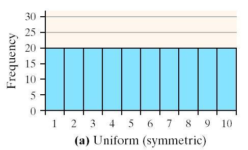
41 Uniform Distribution

42 Symmetric Bell Shaped

43 Skewed Right

44 Skewed left

45 Example Relative Cumulative Frequency Suppose you are considering investing in a Roth IRA. You collect the data table, which represent the three-year rate of return (in percent) for 40 small capitalization growth mutual funds

46 Example Relative Cumulative Frequency Class Freq Relative Frequency Total 40 1 Cumulative Frequency Relative cumulative Frequency

47 Example Relative Cumulative Frequency Class Freq Rel Freq Cum Freq Rel Cum Freq of the 40 mutual funds had a 3 year rate of return of 24.9% or less 65% of the mutual funds had 3 year rate of return of 24.9% or less A mutual fund with a 3 year rate of return of 45% or higher is out performing 95% of its peers.

48 Example Relative Cumulative Frequency L3 Upper Class Limits L4 Relative Cumulative Frequency

49 Example Relative Cumulative Frequency

50 Cumulative Relative Frequency Example Relative Cumulative Frequency 3 Year Rate of Return for Small Capitalization Mutal Funds Rate of Return

51 Lesson 1-2 Describing Distributions with Numbers Measuring the center

52 Mean To find the sample mean add up all of the observations and divided by the number of observations. X x x x n n X x n Is affected by unusual values called outliers.

53 Median The median is the midpoint of a distribution, such that half the observation are smaller and the other half are larger. Another name for the 50 th percentile Is not affected by unusual values called outliers

54 Center and Distribution Mean < Median Skewed Left Mean = Median Symmetric Mean > Median Skewed Right

55 Measuring the Spread Range Quartiles Boxplots Standard Deviation Variance

56 Range The range is the difference between the largest and smallest observation. R x x max min

57 Quartiles Quartiles divides the observation into fourths, or four equal parts. Smallest Data Value Q1 Q2 Q 3 Largest Data Value 25% of the data 25% of the data 25% of the data 25% of the data

58 Interquartile Range (IQR) The interquartile range (IQR) is the distance between the first and third quartiles IQR Q Q 3 1

59 Outliers Upper Cutoff Q 1.5( IQR) 3 Lower Cutoff Q 1.5( IQR) 1

60 Five Number Summary Smallest observation (minimum) Quartile 1 Quartile 2 (median) Quartile 3 Largest observation (maximum)

61 Example Page 41, #1.32 The Survey of Study Habits and Attitudes (SSHA) is a Psychological test that evaluates college students Motivation, study habits and attitudes toward school. A private college gives the SSHA to a sample of 18 of Its incoming first-year women students. There scores are

62 Example Page 41, #1.32 A) Make a stemplot of these data. The overall shape of the distribution is irregular, as often happens when only a few observations are available. Are there any potential outliers? About where is the center of the distribution (the score with half the scores above it and half below)? What is the spread of the scores (ignoring any outliers)? STAT EDIT 1:edit

63 Example Page 41, # is a potential outlier. The center Is approximately 140. The spread (excluding 200) is = 77.

64 Example Page 41, #

65 Example Page 41, #1.32 B) Find the mean. x C) Find the median of these scores. Which larger: the median or the mean? Explain why. Median The mean is larger than the median because the outlier at 200, which pulls the mean towards the long right tail of the distribution.

66 Example Page 47, #1.36 Here are the scores on the Survey of Study Habits and Attitudes (SSHA) for 18 first-year college women: and for 20 first-year college men: A) Make side-by side boxplots to compare the distribution.

67 Men Example Page 47, #1.36 SSHA SCORES Box Plot

68 Example Page 47, #1.36 B) Compute the numerical summaries for these two distributions. x Min Q 1 Median Q 3 Max Women Men

69 Example Page 47, #1.36 C) Write a paragraph comparing SSHA scores for men and women. All the displays and descriptions reveal that women generally score higher than men. The men s scores (IQR = 45) are more spread out than the women s (even if we don t ignore the outlier). The shapes of the distributions are reasonable similar, with each displaying right skewness.

70 Describing Distributions with Numbers Standard Deviation and Variance

71 Standard Deviation The standard deviation (s) measures the average distance of observations from their mean.

72 Example, Page 52, #1.40 The level of various substances in the blood influence our health. Here are measurements of the level of phosphate in the blood of a patient, in milligrams of phosphate per deciliter of blood, made on 6 consecutive visits to a clinic

73 Example, Page 52, # A. Find the mean. x

74 Example, Page 52, #1.40 Observation Deviations Square Deviations x x x i x i x i

75 Example, Page 52, #1.40 x 4.6 x 5.4 x

76 Example, Page 52, #1.40 Observation Deviations Square Deviations x x x i x i x SUM 0 2 (0.2) 0.04 i SUM 2.06

77 Example Page 52, #1.40 B) Find the standard deviation (s) from its definition s xi x n s s

78 Example Page 52, #1.40 C) Use your TI-83 to find x and s. Do the result agree with part B. STAT

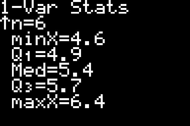
79 Example Page 52, #1.40

80 Standard Deviation Standard deviation (s) is the square root of the variance (s² ) Units are the original units Measures spread about the mean and should only be used when the mean is chosen as the center If s = 0 then there is no spread. Observations are the same value As s gets larger the observations are more spread out. Highly affected by outliers. Best for symmetric data

81 Variance Variance (s²) measures the average squared deviation of observations from the mean Units are squared Highly affected by outliers.

82 How to Choose? Skewed Distribution or Outliers Five number summary Symmetric Distribution or No Outliers Mean Standard Deviation

83 Homework HW, page 52, #1.41, 1.43 Read pages 53 61

84 Linear Transformation A linear transformation changes the original variable x into the new variable x new given by an equation of the form x a bx new Adding the constant a shifts all values of x upward or downward by the same amount. Multiplying by the positive constant b changes the size of the unit of measurement.

85 Example Page 56, #1.44 Maria measures the lengths of 5 cockroaches that she finds at school. Here are her results in inches A. Find the mean and standard deviation.

86 Example Page 56, #

87 Example Page 56, #1.44 B) Maria s science teacher is furious to discover that she has measured the cockroaches lengths in inches rather than centimeters. (There are 2.54 cm in 1 inch). Find the mean and standard deviation of the 5 cockroaches in centimeters. x 1.5 s (2.54) 0.436(2.54) 3.81cm cm

88 Example Page 56, #1.44 C) Considering the 5 cockroaches that Maria found as a small sample from the population of all cockroaches at her school, what would you estimate as the average length of the population of cockroaches? How sure of your estimate are you? The average cockroach length can be estimate as the mean length of the 5 sampled cockroaches of 1.5 inches. This is a questionable estimate, because the sample is so small.

89 Example Page 63, #1.56 A change of units that multiplies each unit by b, such as change xnew x from inches x to centimeters x new, multiplies our usual measures of spread by b. This is true of the IQR and standard deviation. What happens to the variance when we change units this way? Variance is changed by a factor of 2.54² =

90 Homework HW, Page 56, #1.45 HW, Page 63, #1.55

91 1-2 Describing Distributions with Numbers. Comparing Distributions

92 Example Page 59, #1.48 The table below gives the distribution grades earned by students taking the Calculus AB and Statistics exam in Calculus Statistics % 23.2% 23.5% 19.6% 16.8% 9.8% 21.5% 22.4% 20.5% 25.8% A. Make a graphical display to compare the AP exam grades for Calculus AB and Statistics.

93 % of students Earning Grade Example Page 59, # AP Exam Calculus AB Statistics Grade on Exam

94 Example Page 59, #1.48 B) Write a few sentences comparing the two distributions of exam grade. Do you know which now know which exam is easier? Why or why not? The distributions are very similar for grades 2, 3, and 4. The major difference occurs for grades 1 and 5. With a larger proportion of Statistics students receiving a grade of 1 and a smaller proportion of Statistics student receiving a grade of 5. This suggest that the Statistics exam is harder in the sense that students are more likely to get a poor grade on the Statistics Exam than on the Calculus AB exam.

95 Example Page 63, 1.54 The mean x and standard deviation s measure the center and spread but are not a complete description of a distribution. Data sets with different shapes can have the same mean and standard deviation. To demonstrate this fact, use your calculator to find x and s for the following to small data sets. Then make a stem plot of each and comment on the shape of each distribution Data A Data B

96 Example Page 63, 1.54 Set A Set B

97 Example Page 63, 1.54 Set A = 3.1 Set B

98 Example Page 63, 1.54 The means and standard are basically the same. Set A is skewed to the left, while Set B has a higher outlier.

99 Homework HW, Page 59, #1.47, #1.49 HW, Page 62, #1.51, 1,57