Influence of inflow conditions on simulations of arterial blood flow. Marcus Strimell Flodkvist February 14, 2018

Transcription

1 Influence of inflow conditions on simulations of arterial blood flow Marcus Strimell Flodkvist February 14,

2 Contents 1 Introduction 3 2 Method Model Geometry Governing Equations Boundary conditions Data analysis. 7 4 Convergence study Velocities Wall Shear Stress Cycle to cycle variation Results Longitudinal cuts in the descending aorta Geometry, case A Geometry, case A Geometry case A Geometry case A Cross section area Kinetic Energy Normal Vorticity Wall Shear Stress TAWSS OSI Segmented OSI Conclusion 40 2

3 1 Introduction The blood is responsible for the oxygenation of the body and to carry nutrients to the different parts of the body and waste products away from the major organs like the liver, kidneys but also the walls of the arteries. Blood is composed of red blood cells that are on average 45% of the total volume, the rest of the blood is made up of blood plasma platelets, white blood cells, minerals and nutrients. The red blood cells are responsible for the distribution of oxygen and CO 2. To facilitate the distribution of oxygenated blood the circulatory system is used to make sure that blood is reaching the parts of the body. The largest artery in the body is the aorta, which connects the heart to the rest of the body. The aorta is composed of the ascending aorta, the aortic arch and the descending aorta, the ascending aorta have the heart valves connected to it. The descending aorta has two parts the thoracic and the abdominal aorta. The abdominal aorta is in the lower part of the body and bifurcates into smaller arteries that connects to the kidneys and liver. The aortic arch is a bifurcation part that splits the blood flow up into, the Brachiocephalic artery the Left common coronary artery, the Left subclavian artery and the descending aorta. The walls of the aorta is made up of layers so that the aorta can be anchored to the surrounding organs to maintain stability. Leaving the heart, the blood flow features are clearly influenced by the hearth valves as well as the shape of the root. It is the movement of the valves and the following change in pressure and velocity that is one of the underlying mechanism for the observed flow features. As the discharged blood is traveling up the ascending aorta the curved nature of the aorta will affect the flow. The time-varying flow field will result in a shear stress at the wall which under certain circumstances can results in a hardening or build up of the artery wall [5]. The shear on the wall in the descending aorta depends on the inflow condition and the geometry effects on the flow field, both for the aorta and the inflow area. The reason for CFD simulations of the human aorta is due to the high prevalence of cardiovascular decease in the western world with the purpose to further understand the underlying mechanisms responsible thereof. The challenge in such simulations lies in complexity of the circulatory system, making a well-resolved fluid simulation of the entire system not feasible. This is due to the demand of computational power needed to obtain well resolved geometries as well as flow features properly describing the fluid flow. Reducing the model of interest for simulations, leads to another challenge, which is posing the proper boundary conditions. In computational fluid dynamics the boundary conditions are what in part defines the solution, the conditions on the boundaries are a source of debate between accuracy, realism and computational efficiency and here are where the compromises are found and also what is to be simulated. These choices becomes more apparent as the complexities of the physical domain is taken into consideration. In this case there is bifurcations along the domain with outflow conditions that will effect the flow field. So the inflow conditions effect on the solutions are an important aspect when considering the flow field downstream of the boundary. The goal of this report is twofold, firstly it is to simulate the flow field in the aorta for four different cases. With the end goal of in detail investigate the flow field in the descending aorta. Secondly it is to using a simpler geometry and a more complex inflow condition to simulate a more complex geometry. Focus will be placed on the flow field in descending aorta, and how the inflow conditions are effecting flow. The core of the question is how the boundary conditions are effecting the wall shear and the how the disturbances are advected down into the descending aorta. 3

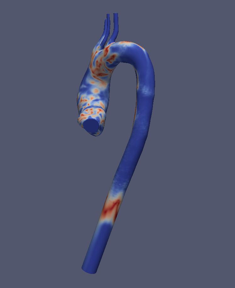
4 2 Method 2.1 Model Assumptions The aim is to investigate how inflow conditions affects the flow in the descending aorta with respect to the quantities used in hemodynamics. This is carried out on patient specific geometries obtained from CT-scans of the aorta. The flow is pulsating which suppresses the growth of the boundary layer, this will shape the flow from a parabolic velocity profile to a flatter profile [9]. The fluid used in the simulation is a non-newtonian fluid, the red blood cell concentration in the flow is being model with a advective diffusion equation. Which is connected to the velocity field. The viscosity model is Quemada model that developed during the 1970 to have a broader range of viscosity than other established models [7]. The pulsating nature of the heart could destabilize the flow and create turbulent flow. There have been studies done that shows that for a normal aorta the flow is not turbulent [6] hence a laminar flow model where used. To ensure that the resolution is fine enough to resolve the flow field a mesh convergence study was performed as presented in section Geometry Two different geometries are investigated in this study, both composed of the ascending aorta, the aortic arch and the descending aorta. The aortic arch have three branches, the brachiocephalic artery, the left common carotid artery and the left subclavian artery located at the same general position for both geometries. (a) Geometry A1. (b) Geometry A2. (c) Geometry A3. Figure 1: The 3 models used. The first patient specific geometry, (A1), is shown in Figure 1a. This geometry is used to evaluate the convergence for the solver. The second geometry is shown in Figure 1b, whose largest difference is the root attached on the inflow boundary. This configuration is closer to 4

5 a realistic aorta. The heart valves are predicted to add complexities to the inflow. A third geometry, (A3), was generated by removing the root from A2, as shown in Figure 1c. Table 1 Case Aorta Inflow Figure 1 A1 plug flow 1a 2 A2 plug flow 1b 3 A3 plug flow 1c 4 A4 Swirl 1c Table 2: Naming the inflow and geometries used in this report. 2.3 Governing Equations The assumption made is the grounds for the choice of equations, and since there is a transport of RBC there is a varying of density and viscosity and therefore the equations to simulate the flow are the Navier Stokes equation with time and spatial varying density and viscosity. D(ρ u) Dt [ ] = p + µ( u + ( u) T ). (1) The density is coupled to the time and spatial position through the hematocrit. Conservation of mass gives Dρ + (ρ u) = 0, Dt (2) ρ = ρ H α + ρ p (1 α), (3) where ρ is the mixture density, ρ H is the density of the RBCs and ρ p is the density of the blood plasma. The transport of RBCs is model by a advection diffusion equation, α t + u α = D H 2 α, (4) where α is the hematocrit and D H is a diffusion coefficient. The viscosity depends on the local shear rate, γ, and the hematocrit in accordance with the Quemada model [7]. ( ) k( γ, α) µ = µ p 1 α (5) 2 k( γ, α) = k 0(α) + k (α) γ/ γ c (α) 1 + γ/ γ c (α) where the variables γ c (α), κ 0 (α) and k (α) are continuous functions Boundary conditions Two different inflow conditions are considered The normal component of the inlet velocity is specified by the volumetric flow rate. Physical flow curves have been obtained from data published in [2]. (6) 5

6 Figure 2: The volume flow profile. The outflow conditions for the branches in the aortic arches are set to have a volumetric flow, of 15%, 7.5% and 7.5% of the inlet flow rate. The outflow for the descending aorta is set to a pressure outlet. These BC was chosen to be a mean pressure conditions to enable possible back flow and to stabilize the numerical solution. The branches on top of the aortic arch are extended to set the outflow as faraway from the bifurcation as possible. For the first geometry, A1, the arteries on top of the arch are pointing in towards each other, this meant that the possible extension are set to be 4 times the averaged diameter. For the cases A2, A3 and A4 the extensions where made to an equivalent length. The boundary-condition for the hematocrit is set to be a constant 45% inflow, and zero-gradient on the rest of the boundaries. On the wall the physical interpretation is that there is no penetration across the aortic wall. The zero gradient across the outflows can be seen as a continuity condition, so there is no discontinuity on the border. Four different simulation are made, whit three different inflow condition as summerized in tabel 3, the first inflow case is shown in Figure 2 which where used on geometry A1, A2 and A3. The Inflow conditions are a volumetric condition so the velocity will be scaled with the area. The inflow case A2 will have a higher velocity at the inflow boundary due to the smaller area. For case A4, there is a special inflow condition imposed, the domain model used is geometry A3. The 4th inflow case samples the flow field from the case A2. The samples are taken downstream of the root. The general idea is to assume that the inflow can be seen as a linear function of a velocity and a solid body rotation. The solid body rotation is taken as the ratio between the angular momentum around the center of the plane and the moment of inertia around the same sampled from case A2. This is to simulate the swirl that the aortic root generates. Explicitly 6

7 the inflow condition is, U in = U ē n + ω(t) r ē θ. (7) Where ω is calculated from the measurement taken from the case with root, the measurements are taken just after where the root ends in Figure 1b and are transient. So this equation is superimposed on the inflow area and ω is acting on the plane around the mean center point of the inflow area. The velocity, U is the velocity taken from the velocity inflow condition. The equations are solved using OpenFoam version 2.3.x with a solver that have been developed at KTH Mechanics, as an extension of a standard solver for multiphase fluid. The solver utilizes a pressure correction with over-relaxation and multigrid approach to speed up convergence. The discretization is done with a FVM-scheme which have the advantage that they ensures that the conservation equations are met. The mesh used is thetrahedral with prism layer at the wall, there to resolve the near-wall flow, since the metrics WSS and OSI are on the wall and the flow is theoretically flowing downstream homogeneously. They are more elaongated in the main flow direction than the core cells. 3 Data analysis. Averaging. To be able to quantify the flow field in the descending aorta, sequential cuts are taken downstream of the aortic arch as shown in Figure 3. The fields are sampled at planes perpendicular to the center-line of the model. The flow in the boundary layer is more sensitive than the flow in the core of the aorta, so the results shown is taken from the core of the aorta. Q k = 1 φ da (8) A tot Where φ is the quantity of interest, either the normal vorticity or the kinetic energy. Shear indices The two different shear indices are time averaged wall shear stress, TAWSS, the oscillatory shear index, OSI [3]. The metric TAWSS is taken over one cycle and is indicates areas of high averaged shear stress and depending on the values could indicate areas of build up on the arterial wall. The results are taken from the third cycle so that the initial effects have been disappeared. T AW SS = 1 T τx,wall 2 T + τ y,wall 2 + τ z,wall 2 dt (9) 0 The OSI has a numerical value between zero to 0.5. Where a value of zero means that the wall shear stress vector is on averaged over the pulse inline with the averaged vector and if the value is 0.5 the vector is oscillating, [3], OSI is often used in arterial flow. [ OSI = 1 1 ] T W SS dt 0 2 T 0 W SS dt (10) A The third shear index is peak temporal wall shear stress gradient [8], Since the flow is tran- Where the values are taken from the third cycle for the simulations. sient the wall shear along the wall will change as the pulse is changing. 7

8 Figure 3: The cut planes in the descending aorta used to evaluate the flow disturbance. 4 Convergence study Convergence To show convergence the first is to investigate mesh independence, which is done for flow case A1. The second is a cycle to cycle difference that shows the difference in volume flow in the descending aorta between the last pulse and the cycle before as a function of time. Q(t) = Q(t + 4 T ) Q(t) (11) The mesh independence study is done by using Richardson extrapolation to get a extrapolated value and then calculating the error between the three meshes used for flow case A1 according with [1]. 4.1 Velocities The accuracy of the results are dependent on the discretization of the governing equations and the mesh cell density. It is thus important to have enough cells in order to obtain an accurate result. To ensure that the results are as independent from the mesh cells density as possible, three simulations were performed with 2,4 and 8 million cells, using consistent outflow and inflow condition to investigate the mesh independence. A cross-section is placed after the last major curvature or the arch, where the highest velocities are found. The largest difference in results should hence be observed there. The velocities are probed along two lines that are perpendicular to each other, line 1 and 2, shown in Figure 4. 8

9 Figure 4: The model with the probe cross-section shown. Table 3: The Richardson extrapolated error values. t = 2.16 Line 1 Line 2 r r p avg (GCI8mil 48 avg 2.18% 4.51% Table 3 the convergence order and the fine grid convergence order, p and GCI respectively. Is given as averages over the time-series and as averages over the probe-lines. And the value are acquired for peak inflow volume. The high order of convergence is due to the relatively low refinement factor. If a higher refinement value, r i,j, was used the order of convergence would be more realistic. The error for the 4 million case is given as 2.2% retrieved using Richardson extrapolation [1]. 9

10 (a) The time mean for the velocity in the x direction. (b) The time mean for the velocity in the y direction (c) The time mean for the velocity in the z direction Figure 5: The mean velocities for Line 1. In Figure 5, the general trend shows good agreement between the meshes with 8 million and 4 million meshes. 10

11 (a) The time mean for the x direction. (b) The time men for the y direction. (c) The time mean for the z direction. Figure 6: The mean velocities for Line 2. As displayed in Figure 6 for the second line there is a similar agreement between the 4 and 8 million meshes. The coarsest mesh i.e 2 million cells and displays the largest difference. Between 11

12 the 4 million and 8 million mesh case the difference in velocity is smaller, which is the important characteristic to show. That as the mesh is refined the difference between them is smaller. The error between the 4 million cell count and 8 million cell count is on average 4.5%. 4.2 Wall Shear Stress The wall shear stress is given in cylindrical coordinates and the normal to the surface shown in the coming figures are on the inner surface of the aortic wall. The components are τ rθ, τ rr and τ rz. 12

13 (a) The spatial mean wall shear stress, τ rθ. (b) The spatial mean wall shear stress, τ rr. (c) The spatial mean wall shear stress, τ rz. Figure 7: The mean wall shear stress for the three different meshes. The reason for using the wall shear stress is to show that the derivative of the velocity field are similar for the three meshes. In Figure 7a there is a general trend of similarity, the large 13

14 change around 50 degrees is due to the re circulation zone that is present. The general trend is that the 4 million mesh follows the 8 million more closely than the 2 million mesh. This is to be expected. What these Figures shown, is that the convergence is not linear, since if it where the different meshes should be stacked on each other. 4.3 Cycle to cycle variation The overall profile is similar, pulse by pulse. The difference is steadily decreasing, that indicates a converging solution. By inspection the convergence is oscillate in nature, the difference is oscillating around a zero level. The calculations are done as by equation (11). (a) Cycle to cycle for case A1 (b) Cycle to cycle for case A2 (c) Cycle to cycle for case A3 (d) Cycle to cycle for case A4 Figure 8: Difference between the last cycle and the earlier cycles, for the four flow cases Figure 8 shows the difference between the volume flow in the descending aorta for the the four flow cases and normalized on the last cycle. The plots shows the difference is decreasing and after just three cycles the difference is around 1% for case A1 and A4. Case A2 and A3 are down around 5% after the fourth cycle, the transient is decreasing for all cases. 14

15 5 Results In this section, results will be displayed for t = 0.2 and t = 0.4 where the first one is in the declaration phase of the flow. The second is close to after the first minimum point for the flow, the flow is starts acceleration again (see Figure 9). Figure 9: The volume flow temporal profile with the times used indicated with circles. The λ 2 -criterion [4] is used to depict the vortical structures in the aorta to give an overall representation of the flow field. It is calculated from the second invariant of the gradient of the velocity field. The second eigenvalue of the gradient of the velocity field is evaluated for every point in the mesh and for every time-step. If λ 2 is less than zero there can be a vortex present in that point. The λ 2 -criterion, and streamlines that are made perpendicular to the flow shows how the flow is behaving downstream. To visualize the λ 2 structure the threshold of was used, positive values where used due to the way λ 2 criterion where calculated. If other values where used either no structures where shown or it showed a noisy pictures. 5.1 Longitudinal cuts in the descending aorta. To examine the velocity field in the descending aorta longitudinal cuts are shown where the difference between the cases A1 and A2 with the three different inflow cases are shown. The scale is between U mag [0, 1.5] meters per seconds, for the time-step at t = 0.2 and U mag [0, 0.3] for the time-step t =

16 Figure 10: Longitudinal cuts along the descending aorta for t=0.2 In Figure 10 the cuts are ordered from left to right as, A1, A2, A3 and A4 respectively. Flow case A1 shows a large even velocity in the descending aorta with a clear area of re-circulation in the beginning of the aorta. For A2 the flow have a lower velocity and the velocity difference is lower between the re-circulation zone and the velocity in that area. This particular trends are the same for the flow cases A2, A3 and A4. Figure 11: Longitudinal cuts along the descending aorta, t=0.4 In Figure 11 the order is left to right flow case A1, A2, A3 and A4. In Figure 11 there is a clear and disturbed flow field which shows a large structure is extending down-stream. The reasons for the more disturbed flow field is likely due to the sharper change in radius as the flow is progressing from the arch to the descending aorta, there is less of a sweep. There are trends that are seen in all three models, A2,A3 and A4, there is an oblate eye like structure, in the upper part. In the same position, there is a dual band like structure in the lower part that is present in all three cases. But there are small details that differentiate the cases from each-other. The bands of higher velocities are narrower and less distinct, which indicates a more graduate change of velocity, in the horizontal direction. Closer to the right wall there is a velocity stratified field 16

17 that is closer in shape. But to the left of this areas there are larger differences, this is dependent on the difference in the upstream velocity field. The general trend taken globally over time shows more of a similarity for the model without the root and with the root, than between the swirly inflow case. For the second geometry the difference in the flow field in the descending aorta is small when the flow is in the deceleration phase. There are noticeable differences for when the flow is accelerating, t = 0.4, but those differences are shrinking as the flow is flowing downstream. The flow for the first geometry is more disturbed for both times shown and there are some clear areas of re-circulation present. 5.2 Geometry, case A1 (a) λ 2 t = 0.2 (b) λ 2 t= 0.4 Figure 12: The first geometry for two different time step. 17

18 Figure 13: Velocity for cut, streamlines indicates the in plane and color is perpendicular velocity. The shear metric λ 2 is shown in the aorta in Figure 12. For the t = 0.2 there is a vortical structure that is created in the arch and reaches downwards into the descending aorta. For this flow case there are vortical structures that are created in the carotid arteries that connects with the ones created in the arch. At t = 0.4 the structure takes up a large part of the descending aorta. Here we can observe a large and connected vortical structure that stretches up into the artier on the arch. The vortical disturbance s are taking up a large part of the aorta, the exception is the ascending aorta. In Figure 13 the left column shows the secondary flow for t = 0.2. For the first cross sectional plane the stream lines shows a parallel behavior, this indicates that the flow have a low level of disturbances, the flow is overall perpendicular to the cross section. The cross section in the first column second row, t = 0.2, there is a circular structures in the upper right area. This indicates that there is a vortical structure through this area, this vortical structure can bee seen in Figure 12a. In this area there is a creation of vorticity. This vorticity that is shown in the third row for t = 0.2 has it nucleus in the arch. And in the last cross section the flow is back to a laminar flow that has flow lines that are perpendicular to the cross section. For the second column in Figure 13 the flow is disturbed in all of the cross sections. Starting low in the first row and then taking up a major part of the cross section in the last three rows. 18

19 5.3 Geometry, case A2. The inflow case is a volumetric inflow case that is called the base case for this geometry, shown in Figure 9. The flow field is then affected by the complex geometry, the geometry is complex in relation to the other geometries at the inflow for the other cases. In Figure 14a there is two areas of vortical creation, in the root, between the first cross section and the inlet, and at the arch. The creation of vorticity at the root is shown to be relatively high and taking up the whole volume between inlet and first cross section. These structures can then be seen a being advected downstream until they reach the aortic arch, seen in Figure 12b. (a) λ 2 after the peak flow, second geometry first inflow case t = 0.2. (b) λ 2 for the second geometry first inflow case, t = 0.4 seconds. Figure 14: The second geometry with A2 inflow case. 19

20 Figure 15: Four cuts along the aorta, the stream lines are in-plane velocity and the color coding is for perpendicular flow. At the arch the arteries on the arch, morphs the flow and changes the characteristic of the flow, there is an gap until the end of the arch seen in Figure 14. Where a new production area is seen, which is a characteristic that the second geometry for this inflow case have in common with the first geometry. In figure 15 the first column shows that the flow have a vortical structures in it at the first cross section. The flow have not had time to transport the structures down stream and hence they are not shown in the second row in the first column. The production of vorticity observed in Figure 15 is not seen for the third row with clarity even though there is a circular pattern in the lower middle corner. That structure is then diffused before it reaches the descending aorta. For the second column in Figure 15 the flow is heavily influenced by the vorticity that has spread downstream from the root. But the volume that the structure takes up is smaller than in Figure 13, and the disturbed parts are shown to end earlier. 5.4 Geometry case A3. Without the root the inflow conditions results in a much calmer flow, the inflow is the base line volumetric flow shown in Figure 9. 20

21 (a) The λ 2 for the time 0.2 (b) The λ 2 for the time 0.4 Figure 16: The two different time steps for the second geometry second inflow case,a3. Figure 17: Four cuts along the aorta, where the streamlines are the in-plane velocity and the color coding is the perpendicular velocity. 21

22 In figures 16b and 16a there is a significant lower level of vorticity in the ascending aorta. Due to the complex geometry at the inflow is not present. In Figure 16a there is an area of vorticity at the arch which is present in Figures 12a and 14a. For the second time-step, t = 0.4 there is a finger of continuous vortical structure than gaps the arch and the ascending aorta. In Figure 16b the vortical structure is seen to extend down the aorta, it extends to the last cross section but it ends in that region. For the first column in Figure 17 the only disturbances are shown in the second row. This cross sectional plane is in the arch of the aorta, and it is in this area that the arch where the second generation for vorticity is. For the third and fourth cross section the flow is particular laminar and the vortical structure dissipate over a short length. In Figure 17, second column the flow is disturbed for the last three cross sections. Where for the second row the flow is starting to form into a dual vortical structure. Due to the non-simple geometry this dual structure newer materialize and dies out. 5.5 Geometry case A4. The inflow case is with and added turning of the in-flow condition to try to more closely resemble the second geometry with the first inflow case. (a) The flow field for the second geometry third inflow case, t=0.2. (b) The flow field for the second geometry third inflow case, t=0.4 Figure 18: The overall pictures for two time-steps, t= 0.2 and t= 0.4, inflow case A4. 22

23 Figure 19: Four cuts along the aorta, where the streamlines are the in-plane velocity and the color coding is the perpendicular velocity. The flow field for figure 18a shows the disturbance shown by the aortic arch in the previous cases. There is some small perturbation seen in the ascending aorta that also can be seen in figure 16a so it is not dependent on the swirl from the inflow. As the time is progressing the flow in the ascending aorta have trends that are seen in figure 16b. The oblong structure that starts in the ascending aorta and stops in the descending aorta. It has a larger diameter than in the non-swirl case, and there is a bifurcation of the oblong structure at the top of the arch. The swirl added to the inflow is seen for the time-step 0.4, in the first cut there is a clear turning of the velocity field, this is seen throughout the cross sections in figure 19. For time-step, t = 0.2, the flow field is similar to non-swirl case. For the last flow case, A4 the basic idea of adding swirl to the inflow has its merits but there is a difference between the inflow condition for figure 19 and figure 15. The swirl case have a turn on the velocity field that have a constant direction, and that there is only one major turning motion in the inflow. This difference is a major actor in the flow fields behavior, there is only one point that indicates a swirl. In the case with the root, case A2, there is an irregular pattern of concentric circles, and this pattern is missing for case A4. Using the measurements from the simulations with the root have some limitations in hope of finding a realistic flow field. Since the root is more than likely a source of vorticty in more than one direction, so adding it to the radial and theta direction would be one way of alleviate the unrealistic flow field. 23

24 5.6 Cross section area The solver is using the full mass conservation equation, so theoretically there is a dependency on both time and space for the density. But since the boundary condition for the volume fraction, α is constant in and out there is no change and hence the density is constant. Therefore practicality the flow is incompressible. The cross sectional area which is shown in figures 20. All two cross sectional areas are changing downstream. Due to mass conservation this means that as the area is changing, the velocity needs to change to compensate to make sure that the flow is divergence free. (a) First geometry, A1. (b) Second geometry,a2-a4. Figure 20: The area distribution in the descending aorta for the two geometries. What should be observed is the difference in area at the end of the aorta. The cross sectional area for case A1 is 75% less than the second geometry. Due to this the flow is obtaining in a higher kinetic energy. 5.7 Kinetic Energy In Figure 21 the average kinetic energy is shown over the cross sectional planes. In the time domain there is a periodicity due to the pumping nature of the inflow condition. Since the inflow 24

25 Figure 21: The mean times energy for the flow cases A2-A4. profile is so dominating for the flow, the temporal profile is directly correlated with the kinetic energy. The common trends for the three models are that the kinetic energy is growing, the underlying mechanism is the conservation of mass. From the arch and downwards the cross section is narrowing, this will results in a increase of the velocity. The kinetic energy is growing asymptotically towards a level, which is dependent on the geometry of the model. 25

26 Figure 22: The time mean of the kinetic energy for the first geometry, A1. The energy development for the first geometry, A1, figure 22, is growing. This can be explained from the cross sectional area for the aorta, in Figure 20a there is larger area in the beginning of the aorta. Which correlate with the lower kinetic energy in Figure 22. Furthermore the first geometry, A1, have a decrease in cross- sectional area, so the increase of kinetic energy is due to a decrease in area. Comparing Figure 20a and with Figure 22 there is a clear connection between the area decrease and the increase in kinetic energy. For case A2, there is a steep increase of kinetic energy along the descending aorta. There is a lower range of kinetic energy than in comparison with the first geometry,a1, Figure 22. This comes from the difference in geometry, the second geometry has a more sweeping geometry and the arch goes more seamlessly transition from the arch to the descending aorta. As shown in figure 20b there is some wiggling of the cross sectional area that affects the kinetic energy directly. There is phenomena that is seen in Figure 21 that the kinetic energy changes around a point halfway along the aorta. Case A2, have a higher kinetic energy and after half way the kinetic energy is lower than the two other cases. But the difference in the end of the descending aorta is small for the second geometry. The energy is almost three times the energy level in the end for the first geometry due to size difference between the two geometries. 26

27 (a) The contour plots for A1. (b) The contour plots for A2. (c) The contour for A3. (d) The contour plot for A4. Figure 23: The contour plots for the kinetic energy for the two geometries four inflow cases, A1-A4. In Figures 23b- 23d the kinetic energy shows similar trends for the evolution along the aorta and in time. There are some differences but they are difficult do discern in these plots between the inflow cases for the second geometry. After t 0.3 there is a low change of the kinetic energy that is continued until the next pulse it starting. For Figure 23a there is a narrow waist that can be correlated to an enlarging of the cross sectional area. Which makes the velocity decrease. This decrease is also why the time it takes for the flow to reach a peak energy is longer than for the second geometry. A common trend for Figure 23 is that there is no changed shown for either geometries after t 0.3 this is due to the relative small change in energy levels after that time and until the next cycle. Even though the inflow conditions for the first geometry,a1, is the same for second geometry third inflow condition, A3. The volumetric inflow condition is the same for case A1 and A2 but due to the difference in inflow geometry the initial velocity is higher for A2. Even though this is present in the velocity field the kinetic energy is twice for A1 in comparison to A2-A4. The difference in the kinetic energy between the two geometries are mostly effected by the geometry. 5.8 Normal Vorticity The normal vorticity quantifies the amount of rotation around the center of the plane. The important quantity is whether the values are changing around the zero-line, a positive value 27

28 mean that there is a counterclockwise movement around the center of mass. If the values are changing between positive and negative the flow is more unstable then without the sign change. If the figures shows a change in value but no sign change there is just a magnitude difference. The general trend for the first geometry is that there is a larger value. In the end of the aorta there is still a high normal-vorticity as compared with the second geometry. Figure 24: The normal vorticity for flow cases A1-A4. The vorticity curves follow eachother downstream of the aorta. In Figure 24 (case A4), a higher level of vorticity is observed which is to be expected since swirl is added at the inflow. The overall trends for the cases A2-A4 are the same although they differ in magnitude. The interesting trend to notice in Figure 24 and Figure 21 is that case A2 ends at the lowest level at the end of the aorta. Comparing the first geometry, A1, and the second geometry,a2-a4, there is a large difference in vorticity levels. The general difference in behavior over the aorta is due to the sharp changes in the geometry. 28

29 (a) The contour plot for A1. (b) The contour plot for A2. (c) The contour plot for A3. (d) The contour plot for A4. Figure 25: The contour plots for the 4 simulations, A1-A4. In Figure 25a, there is a structure that is forming close to the left lower corner, and has a right lean, so the structure is moving towards the right. The structures looks to delimited the area, the structures to the right of it seems to have it origin. So the structured is smeared out as it is transport away to the right. This would indicate that there is a large production of voriticity at the end of the arch, that is transported down the aorta. The right leaning structure has a smearing effect parallel to the horizontal axis. But there is also a production of vorticity since there is a horizontal structures that is spreading outwards to. In Figure 25b there is a structure that has it origin at time 1.6 which coincide with the peak volume inflow, and the vorticity is transported away. The vorticity is less peaky than in Figure 25a which is consistent with the Figure 24. At the end of the aorta there is smearing of the vorticity that diffuses away. For Figure 25c there is no clear case of advection of the vorticity downstream, there is a small tendency of it but it is not a clear case. What is more clear is that there is a production of vorticity along the aorta that seems to stay in place. For case A3 there is more of a transportation of vortical structures downstream, but there is more of a mending between the case with the root and the root less case. So for this case there is closer to the case with root. But the transportation is not as strong as in Figure 25b. There is clearly shown that the first geometry have a large difference in vorticity that is not seen for the second geometry. The second geometry first inflow case is closer to a real example 29

30 of the four cases, there are some similarities for between the vorticity in Figure 25d and Figure 25c, but the former have a more of a patchy qualitatively behavior. 5.9 Wall Shear Stress TAWSS The shear indices used in this report are TAWSS, time averaged wall shear stress, and OSI, oscillatory shear index, which shows trends for the shear at the wall. The indices are calculated over the third period. 30

31 (a) The TAWSS for case A1. (b) The TAWSS for case A2. (c) The TAWSS for case A3. (d) The TAWSS for case A4. Figure 26: The TAWSS for the four simluations. 31

32 The results for the first geometry shows a patchy pattern in the descending aorta (see Figure 26a). The TAWSS is around 5P a, in the descending aorta. In comparison to case A2,A3 and A4 it is double the TAWSS of the first geometry. For the case A2 the TAWSS is half the value than for case A1. For case A3 there is a similar pattern in the descending aorta, that is where the walls are clouded over with a TAWSS around half that of A1. There is more of a patchy pattern in the ascending aorta for the the case A2, this comes from the shape of the wall, which incorporates the heart valves. For the TAWSS index in for case A2, shows a high-value in the bend after the aortic arch. This is a natural area of high shear stress since this is after the supra aortic arteries which will morph the flow field, the boundary conditions are set to a percentage of the inflow. So the supra aortic arteries are changing the flow, both adding complexity to the flow and removing mass. There is a higher TAWSS value in the ascending aorta for case A2. This comes from the fact that there is a more complex geometry, so the flow along the root-wall have a large change in direction. So naturally there is going to be a higher TAWSS. The behavior for the TAWSS, in Figure 26b, is continuous with a relative low value along the main aorta. For the arteries on the arch the value is increasing. They were put to a constant volume outflow which means that no matter the physics before the outflow, there should be a certain volume-flow at the boundaries. Which means a higher velocity since the cross sectional area is small. The root adds TAWSS to the ascending aorta since the complexity of the root will shear the flow. In figure 26c there is shown a high level of TAWSS in the supra-aortic arteries and in figure 26b. This is due to the narrowing of the tubes, when the flow is going into the arteries to maintain the volume flow the velocity has to increase. This means that there is a level of shear due to changes in velocity, that is bounded by the shape of the model and not the flow. This could be indicative of future changes or strain that the geometry and tissue have to compensate for, but that is tied to the characteristic of the artery wall and that problem can not be seen in this simulation. In comparison between the swirl case, figure 26c and the non swirl case, figure 26d, the difference are smaller than what is expected to the time averaged wall shear stress. This could be from the fact that the swirl, turning of the fluid field is not large enough to effect the wall shear stress. The general trend in the descending aorta for the TAWSS is a similarity. This similarity starts in the arch, but the ascending aorta is heavily influenced by the inflow conditions. 32

33 5.9.2 OSI The second metric used is the OSI this shows the relative alignment between the shear stress and averaged wall shear stress vector. The theory is that high value of time averaged wall shear stress and low oscillatory shear stress index indicates a probable development of atherosclerosis, 33

34 (a) The OSI for case A1. (b) The OSI for case A2. (c) The OSI for case A3. (d) The OSI for case A4. Figure 27: The OSI for the four simluations. 34

35 In Figure 27a the general pattern is patchy for this metric. Where the high values on top of the arch are placed close to the bifurcations and on the descending aorta the sport are close to the re circulation zone. The high OSI value observed on the root, figure 27b, is just because the major effect the pulsating inflow condition have on the metric. The high OSI value at the base of the arteries at the arch are larger in figure 27b than in figure 27c this size difference is due to the added disturbance that can be seen for the case with root. The high value are due to the two different flow conditions that are meet in the bifurcation. The outflow condition are set to be a percentage of the flow at the boundary, this means that the flow is changing direction a few times under a phase to meet the condition. With the swirl added, Figure 27d there is an increase OSI in the ascending aorta in comparison to the non swirly case. So the inflow condition with the added solid body rotation makes the wall shear stress more oscillatory. But this added swirl is not effecting the descending aorta, so the arteries on top of the arch is subtracting and calming down the wall shear stress. And the OSI at the bifurcation for the first arch artery show a smaller OSI value. It does not totally extinguish the high concentration of OSI found on the front of the ascending aorta. For cases A2 and A3, the OSI have a longitudinal structure that winds it self down on the inside of the aortic arch and the descending aorta. The OSI along the structure is close to 0.5, which indicates that the shear stress is misaligned to averaged flow. This should indicate that there is a re-circulation zone along the inner side of the aorta. There is also zones of disturbance at the top of the arch which is caused by the geometry. The high OSI is shown in all three models. The high OSI in fig 27c on the outside of ascending aorta is due to that patch is placed right in front of the inflow, so the wall shear stress vector will be directly influenced by the pulsating inflow. In comparison between figure 27b which have a higher level of change in the ascending aorta than in figure 26c. But the difference in the descending aorta are smaller, this shows that the arteries on the aortic arch make the flow more homogeneous, since the outflow conditions are the same for two cases. 35

36 5.9.3 Segmented OSI. The OSI is a averaged taken from the wall shear stress, and there is a possibility that some information is lost in the averaging process. To see if there something lost one cycle where segmented into 5 segments. This allows us to identify where in the cardiac cycle flow disturbances occur in different parts of the aorta. Figure 28: The volumetric inflow profile. General trends There are some general trends that are directly evident. The averaging for the OSI results in a lower value in the descending aorta. The initial OSI time segment shows a low numerical index value for the cases without root. The last time step shows a high value in the descending aorta. there is a high oscillaoty flow in the descending aorta. There is a apparent transport of OSI as the time is progressing. Geometry A1. There are some difference between Figures 29 and Figure 27a. The largest is for time segment 5 which have a large structure in the descending aorta, that has a large value. And then looking at the descending aorta for Figures 29a, 29b, 29c and 29d where the values are low. The duration of the time for Figure 29e is 0.2 seconds which is 20% of one pulse, so a significant time period. Geometry A2. Initially the index can be seen growing with the nucleus from the root. The index looks to be growing and transporting from the root down the aorta. Where certain areas 36

37 seems to have a production after the initial wave have past. This is shown in the outflow arteries on the top of the arch. The same behavior can be observed when OSI is time segmented, the first four segments have a small OSI in the descending aorta but in Figure 30e there is a substantial OSI. Geometry A3. There is structures that is artifacts of the inflow condition that is seen as a ring in the descending aorta for Figures 31c and Figure 31e. These structures are also present in Figure 32, this would indicate that the planar inflow condition used is not strong enough to change the flow field to any degree. Geometry A4. There is a band in the ascending aorta for all 5 time steps. This is an artifact from the artificial boundary condition. The flow features in the descending aorta shows similarities between case A2 and A3, see Figure 30 and 31. Looking at the ascending aorta the flow features shows similarity with case A3, Figure 31. With a large area of high OSI on the front of the ascending aorta as seen in the second time segment, Figure

38 (a) Segment 1 (a) Segment 1 (b) Segment 2 (b) Segment 2 (c) Segment 3 (c) Segment 3 (d) Segment 4 (d) Segment 4 (e) Segment 5 (e) Segment 5 Figure 29: The OSI time segmented for Figure 30: The OSI time segmented for case A1. case A2.

39 (a) Segment 1 (a) Segment 1 (b) Segment 2 (b) Segment 2 (c) Segment 3 (c) Segment 3 (d) Segment 4 (d) Segment 4 (e) Segment 5 (e) Segment 5 Figure 31: The OSI time segmented for Figure 32: The OSI time segmented case A3. for case A4.

40 6 Conclusion The aim for this is to investigate how inflow conditions affects the flow field in the descending aorta, including physical quantities tied to the flow field, vorticity and kinetic energy. Furthermore the feasibility of modelling the influence of the root as a solid body rotation was considered a solid body rotation would mimic the more complex flow of a simulation with the root attached to the aorta. The velocity field for the flow cases are similar, certain flow features are in place for the similar geometry. The re-circulation at the end of the arch being a nucleus of helical structure that is advected down the aorta. There are larger differences between A1 and A2,A3, A4 and this is due to the difference in geometry. The normal vorticity trends to a similar value, the difference is around 2 3% at the end of the aorta. This is due to the vorticity is strained in the aortic arch, the level of vorticty is lowered and then produced again in the latter end of the aortic arch. This is a phenomena that is present in all four cases to a lesser or higher degree. For flow case A2 there is a noticeable dip between the middle of the arch and the end. But the for A1,A3 and A4 there is a structure that connects the flow between the descending and the ascending aorta through the arch. The general trend for the kinetic energy is heavily correlated with the geometry of the domain. Since the flow is incompressible and the walls are rigid. The incompressibility condition is the physical effect that results in this correlation. The use of the shear indices shows a similar trend that is indicated by the velocity, vorticity and kinetic energy. That the trends and overall look of the descending aorta for cases A2,A2 and A4 are similar. The largest difference between flow case A1 to A2,A3 and A4 is the geometry of the two forms. The noticeable difference is in the ascending aorta where the geometry of A2 is completely different from A3 and A4. And it is here that the major differences are seen for the three shear indices. The root geometry of the walls is influencing the wall shear stress. So whether or not the place of high OSI and low TAWSS is important comes down to how the rigid wall approximation effects the solution, since a deform-able arterial wall will make the area time and velocity dependent. Which will modify the governing equations. The second part of the goal for this report is to investigate if it was possible to simulate a complex inflow condition with a simpler flow case, can the effects from A2 be simulated in case A4. In case A4, the results are overall different for this case. This is more than likely due to the measured secondary flow is to low to create any meaningful vortical and velocity structure. The largest discrepancies for the two flow cases are down to the complex flow that the root in case A2 can create. This blooming effect, due to the geometry, shows that the initial disturbances that are created are of a small scale. What can be seen in for the shear indices is that the blooming effect in the ascending aorta is not present for case A3,A4 and A1. The effects from the inflow conditions are dependent on the proximity to the inflow boundary. The largest effects from the inflow conditions when the shear indices considered are in the ascending aorta. The shear behavior in the descending aorta is similar and this is due to the similarity of geometry, the influence of the inflow conditions have by that place died down. The similarities for the descending aorta when the kinetic energy is considered is that the geom- 40