Flow in Pipes Simulation Using Successive Substitution Method

Transcription

1 Flow in Pipes Simulation Using Successive Substitution Method Dr. Ismail Al-Rawi Arab Open University, (Kuwait Branch), P.O 830 Al Ardia, P.C 92400, Kuwait Abstract The aim of this paper is to present the implementation of mathematical model to simulate the flow of fluid and gas in pipes network consisted of a number of horizontal pipes of specified diameters and length, joined at a number of nodes, and to compute the pressure, the flow rate, and the direction of flow at each node. Such simulation allows predicting the behavior of the fluid network system under different conditions. Such prediction can be effectively used to give decisions regarding the design and the operation of the real system. This model adopt the successive substitution method as a numerical technique to solve non-linear equation using a fixed-point iteration. Keywords: Flow in Pipes Network, Successive Substitution Method, Numerical Methods, Fixed Point Iterations. 1. Introduction Fluid flow in pipes is much encountered in our daily life and industry. The hot and cold water that we use in our homes is pumped through pipes. Water in a city is distributed by extensive piping networks. Oil and natural gas are transported hundreds long distance by large pipelines. In our body, blood is carried out by arteries and veins. The cooling water in an engine is transported by pipes in the radiator where it is cooled as it flows. Thermal energy is transferred to the desired locations through pipes. [1] There are many good modules around to simulate the flow in pipes, but our aims here is to find a module, which depends on a simple and efficient mathematical concepts that can be programmed and computed easily. The modules has to counts for time-dependent change in the state of the system and counts all parameters in a continuous manner. [2]. choosing the iterative technique is the key point of the solution methods, and always should answer two basic questions: first, does the iteration converge?. Second, if so, how fast does it converge?. The first question is more important to be answered, in one sense it can be answered easily, and in another too hard to be answered. It is easy to be answered simply because there is a little difficulty in showing that if the initial approximation(s) α of F(x) = 0 are sufficiently close to the root, the iteration will converge to α. In few cases, the iteration will converge to the root independent of the initial approximation. The hard part of answering the question comes from the phrase sufficiently close or how close to the root that is generally depends on the derivative value of f(x) at some unknown points on the interval spanned by the initial approximations [3]. In practice, to ensure the convergence, enough priori knowledge of the desired root is needed. When the prior knowledge is poor, it is recommended to use a method, which converges independent of the starting value until a good approximation is obtained and then switch over to a more rapidly converging method. Solving a system of nonlinear equations is a problem that is avoided when possible, customarily by approximating the nonlinear system by a system of linear equations. When this is unsatisfactory, the problem must be tackled directly. The most straightforward approaches to adapt the methods, which approximate the solutions of a single nonlinear equation in one variable, to apply when the single-variable problem is replaced by a vector problem that incorporates all the variables. [4]. The principal tool to solve the non-linear equations was found in many methods mainly Newton-Raphson method, a technique that is quadratically convergent. This technique has a number of drawbacks. It is quite costly to apply. Poor convergence characteristics when division by zero occurs for some values of the roots. Divergence at inflection points, the method may start to diverge away from the root and it may start converging again to the root. In some case where the function f (x) is oscillating and has a number of roots, one may choose an initial guess close to a root. However, the guesses may jump and converge to some other root. (5). The Other well-known method to solve the non-linear equation is the bisection method, which is One of the first numerical methods developed to find the root of a nonlinear equation (also called binary-search method). It is based on finding the root between two points; therefore, the method falls under the category of bracketing methods. The advantage of this method is always convergent. Since the method brackets the root, the method is guaranteed to converge. As iterations are conducted, the interval gets halved, so one can guarantee the error in the solution of the equation. A number of drawbacks are also found. The convergence of the method is slow as it is simply based on halving the interval. If one of the initial guesses is closer to the root, it will take larger number of iterations to reach the root. [6]. Other methods like false-position and secant method are also used as alternate methods to solve a nonlinear equation, but also a number of drawbacks are exist. [7][8]. 2. Method of solution Our engineering principles are simulated by solving a non-linear functional equation consisted of n real functions 7

2 with n unknown real variables such as: f 1 (x 1, x 2, x 3 x n) = 0 f 2 (x 1, x 2, x 3 x n) = 0... f n (x 1, x 2, x 3 x n) = 0 If we say x = [x 1, x 2, x 3 x n] t then we shall write f i (x) = fi (x 1, x 2, x 3 x n) when 1 i n. This will lead to solve equation in the form of x i = F i (x) such that x = g(x). The method of solving x = g(x) which we shall investigate is that of SUCCSSIVE SUBSTITUTING or Fixed point Iteration Method [9]. Iteration is a fundamental principle in computer science. A process is repeated until an answer is reached. Iterative techniques are used to find roots of equations, solutions of linear and nonlinear systems of equations, and solutions of differential equations. To start the iteration, a function g (x) for computing successive terms is needed, together with a starting value P 0. Then a sequence of values {p k} is obtained using the iterative rule p k+1 = g (p k). The sequence has the pattern of the following: P 0 (starting value) p 1 = g (p 0) p 2 = g (p 1) p k = g (p k-1) What can we learn from an unending sequence of numbers? If the numbers tend to a limit, we suspect that it is the answer [10]. A fixed point of a function g (x) is a number p such that p = g (p), so it is not a root of the equation x = g (x), it is a solution of the equation x = g (x). Figure-1 show the fixed points of the function g (x) as the intersection of the curve y = g(x) and the line y = x. Figure-1 Figure-2 Figure-2 shows how the Fixed Point Iteration works. Let p 0 approximate a solution for the equation x = g (x). Generate the sequence {p n} recursively by the relation p n = g (p n-1), n= 1, 2, 3....that may converge to the root α, and may be shown by Figure-3. We also notice that the root of x = F(x) can be expressed by lim x n = x. Figure-3 8

3 3. Problem statement A network consists of a number of horizontal pipes, of specified diameters and lengths, that are joined at n nodes, numbered I = 1, 2, n. The pressure is specified at some of these nodes. There is at most a single pipe connected directly between any two nodes. We wrote a C program that will accept the above information, and will proceed to compute: (a) the pressures at all remaining nodes, and (b) the flow rate (and direction) in each pipe. 4. Simulation Principles For flow of a liquid from point, I to point j in a horizontal pipe the pressure drop is given by the Fanning equation: Here f M is the dimensionless Moody friction factor, P is the liquid density, u m is the mean velocity, and Land D are the length and diameter of the pipe, respectively. Since the volumetric flow rate is Q = (πd 2 /4)u m, equation (1) becomes: Here, all quantities are in consistent units. However, if P i and P j expressed in psi (Ib f / sq in.), p in (Ib m / cu ft), Q in (gallons / min), L in ft, and D in inches, we obtain: Where If C ij = CL ij l D ij5, where the subscripts ij now emphasize that we are concerned with the pipe joining nodes i and j. The flow rate Q ij between nodes i and j is then given by: in which Q ij is plus or minus for flow from i to j or vice versa, respectively. In the following version, Q ij will automatically have the correct sign: At any free node j, where the pressure is not specified, the sum of the flows from neighboring nodes i must be zero: When applied at all free nodes, equation (5) yields a system of nonlinear simultaneous equations in the unknown pressures. We shall solve this system by the method of successive - substitution. First, we note that ( p i - p j ) is more sensitive than ( p i - p j ) 1/2 to variations in p j. Thus an appropriate version, analogous to equation x i = F(x) is: 9

4 In which Equation (6) is applied repeatedly at all free nodes until either each computed pressure p j does not change by more than a small amount ϵ from one iteration to the next, or a preassigned number of iterations, itmax, has been exceeded. The most recently estimated values of p i will always be used in the right-hand side of equation (6). In order to implement the above, we also introduce the following: (a) A vector of logical values, p 1, p 2.. p n ( PGIVEN in the program ), such that p j is true (T) if the pressure is specified at node j and false (F) if it is not. (b) A matrix of logical values, I I nn (the incidence matrix INCID in the program), such that I ij is true if there is a pipe directly joining nodes i and j, and false if not. Since the incidence, diameter, and length matrices are symmetric (for example D ij = D jj) we need to supply only the lower triangular portions of such matrices as data. The input data will also include a complete set of pressures, p 1, p 2,... p n; some of these will be the known pressures, and the remainder will be the starting guesses at the free nodes. 5. Simulation Methods and Programming Notes Figure-5 represents the flowchart that show the simulation process that are implemented in C-Program which reads a description of the topology of an arbitrary n node pipe network with pressures specified at particular nodes, and then computes the pressures at the remaining nodes and the inter-nodal flow rates using a method of SUCCESSIVE SUBSTITUTIONS. List of used variables and Program Symbol Definition A Matrix, whose elements a ij are defined by equation (7). C Matrix, whose elements c ij relate the flow rate to the pressure drop in the pipe joining nodes i and j. CONV Logical variable used in testing for convergence, conv. D. L Matrices, whose elements D ij and L ij give the diameter (in.) and length (ft) of the pipe joining nodes i and j. DENOM Storage for the denominator of equation (6), den. NUMER Storage for the numerator of equation (6), num. EPS Tolerance, ϵ, used in testing for convergence. F Moody friction factor, f m (assumed constant). FACTOR The constant, c, in equation (3). I.J Indices for representing the nodes i and j. INCID Matrix of logical values, I; if I ij is T, there is a pipe joining nodes i and j; if F, there is not. ITER Counter on the number of iterations, iter. IPRINT Logical variable, which must have the value T if intermediate approximations to the pressures are to be printed. ITMAX Upper limit on the number of iterations, itmax. N Total number of nodes, n. P Vector of pressures, p i (psi), at each node. PGIVEN Vector of logical values, p i at each node. If P i is T, the pressure is specified at node i; if F, it is not. Q Matrix, whose elements Q ij give the flow rate (gpm) from node i to node j. RHO Density of the liquid in the pipes, p (lb m / cu ft). SAVEP Temporary storage for old pressure p, during convergence testing, p. If INCID(I, J) is true, then nodes I and J are connected by a pipe segment of diameter D(I,J) inches and length L(I,J) feet. If PGIVEN(I) is true, the pressure at node I, P(I) psi, is fixed. Otherwise, P (I) assumes successive estimates of the pressure at node I. rho is the fluid density in lb/cu ft and f is the pipe friction factor, assumed identical for all pipe segments. ITER is the iteration counter. Iteration is stopped when ITER exceeds ITMAX or 10

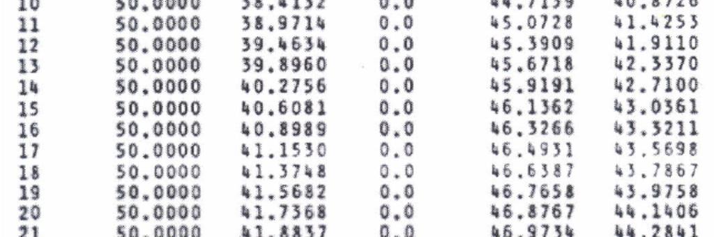
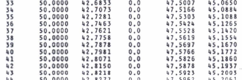
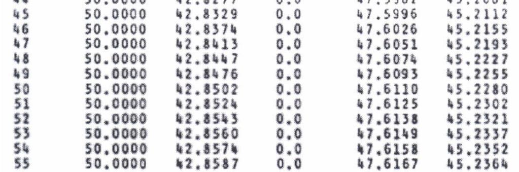
5 when no nodal pressure changes by an amount greater than EPS psi between two successive iterations. Q(I,J) is the flow rate in gal/min between nodes I and J. when Q(I,J) is positive, fluid flows from node I to node J. When IPRINT is true, intermediate approximations of the nodal pressures are printed. 6. Discussion of Results The initial data used in the simulation is shown in Figure-6 and relate to the network that shown in the Figure-7, with f m = 0.056, p=50 Ib m / cu ft, and two pressures fixed p1 = 50, p3 = 0 psi. Results of simulation Figure-8 show that, although the method is computationally straight forward, it needs many iterations to give a reasonable degree of convergence. In addition, referring to equation (7), we can see that a starting guess of p i = p j for any two nodes that are directly connected would be unfortunate. We also note that most of the pressure drop occurs in the pipe 2-3, and that the flow in the branch is appreciably greater than that in the pipe 1-2, even though the latter is much shorter Figure-8. Both these observations can be reconciled by noting that pressure drop is proportional to Q 2 / D 5, and that pipe 2-3 must take the combined flows along and Conclusions The difficulty of using successive substitution method in solving a non-linear equations depend on the nature of the problem, there is no general recognized best method of solution. In our simulation, the method proved to be a powerful method for solution if the approximate locations of the root is known. The success of the method depends on arranging matters so that large errors in an unknown tend to produce smaller ones in the next cycle of iteration. Thus, the successive substitution method is more suitable only when the situations carefully analyzed and details should be easily worked out for any particular situation. The method can be extended to more complex situations, in which we could allow for (a) f m being a function of Reynolds number and pipe roughness, instead of being treated as a constant, and (b) pumps and valves in some of the branches, etc. In addition, the logical arrays used above could find a similar application in solving for the currents in a network of resistors, with known voltages applied at some of the nodes (although this would lead to a set of simultaneous linear equations). References [1] Flow in Pipes. Cen72367-ch08.qxd, Page 321. [2] Bader. E.A.: An Introduction to Mathematical Modeling. N.Y. Dover. ISBN X [3] Anthony Ralston: A first Course in Numerical Analysis. Dover Publication INC, 2001 (Second Edition). [4] J. D. Faris, R. Burden: Numerical Methods. 4 th Edition, ISBN [5] A. Kaw: Newton-Raphson Method of Solving Nonlinear Equation. Text Book, December www. numericalmethods.eng.usf.edu. [6] A. Kaw: Bisection Method of Solving Nonlinear Equation. Text Book, January www. numericalmethods.eng.usf.edu. [7] D. Nguyen: FALSE-Position Method of Solving Nonlinear Equation. Text Book, September www. numericalmethods.eng.usf.edu. [8] A. Kaw: Secant Method of Solving Nonlinear Equation. Text Book, December www. numericalmethods.eng.usf.edu. [9] Al-Rawi: Finding the flow of fluid in pipes Network. Al-Mansour University College Baghdad-Iraq, May [10] Mathews: Module for Fixed Point Iteration. California State University Fullerton. Mathfaculity.fullerton.edu/Mathews/n2003/fixedpointmod.html. [11] Brice C., H.A. Luther: Applied Numerical Methods. Krieger Publishing Company, Malabar, Florida,

6 Figure-5 12

7 INITIAL INFORMATION ABOUT NETWORK TOTAL NUMBER OF NODES=5 THE NUMBER OF ITIRATIONS=100 DENSITY OF THE LIQUID= TOLARANCE= MOODY FRICTION FACTOR= PRESS ANY KEY TO CONTINUE... Figure-6 Figure-7 13

8 Computer output (continued) 14

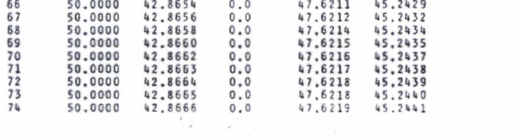
9 Figure-8 15