Model of Motor Neural Circuit of C. elegans

Transcription

1 Model of Motor Neural Circuit of C. elegans Different models for oscillators There are several different models to generate oscillations. Among these models, some have different values for the same parameters, while some other have totally different parameters, or even totally different dynamic equation. It seems necessary to review the three main models of oscillators: Sherman s model in 199, Manor s model in 1997, and the model in the textbook Dynamical Systems in Neuroscience (referred as dsn from now on). The dsn model has two classes of firing. Class 1 can transfer input current to firing frequency continuously, and has a relatively low threshold of firing. Class has a discontinuous f-i relationship, and the threshold of firing is higher. Dsn model Specifically, this model is the model given in chapter 4 of dsn, but not the one in chapter 10. As for Class 1 firing, oscillators composed of two neurons always fire in phase, no matter how strong the gap junction (quantified as gc) is. On the contrary, Class firing can generate oscillators with a particular phase difference, whose value is dependent on gc, I (input current). In order to generate anti-phase oscillators, other parameters also need to be fine-tuned. Shown below are firing pattern and the phase trajectory of Class 1 of dsn model. The threshold input current in Class is between 10 and 0. Given other parameters, the phase difference in the steady oscillating state is dependent on I and gc, as shown in figures below. It is noteworthy that when I=50, the phase difference can be fixed, but neither in-phase nor anti-phase, which is not observed before, and not mentioned in chapter 10 of dsn.

2 When I=50, the two neurons first fire synchronically, but out of phase after a small perturbation of 0.3mV at 50ms to one of the neurons. This process can be verified by the phase trajectory below. Obviously, in this case, synchronically oscillation is not stable. The Sherman model in 199 can generate anti-phase oscillation, we will show later that Sherman model and dsn model are actually equivalent, except for different parameter values.

3 Manor s Model in 1997 This model cannot generate unsynchronized oscillator. Compared to dsn model, this model has three main difference: The two neurons are not the same. Before coupling, one of them is steady and the other one is firing. The ion channels, or specifically, the possibility of opening of the ion channel, is expressed in a different way. The time constant of the parameter of ion channel (for example, the n in dsn model) is not a constant any more, but dependent on V instead. In this model, when gc is small, the two neurons will not fire. And larger gc will lead to synchronized firing only. Sherman s Model in 199 This model can generate anti-phase oscillator if gc is chosen appropriately, as shown in the figure below. In fact, this model can be transformed into dsn model, based on the corresponding relationship listed below. Dsn model Sherman model τ(v) τ/λ n n m C g L g Na g K E Na E K, E L I n n m τ g S S g Ca g K V Ca V K I

4 Linear model for the motor neural network of C. elegans We developed a linear model for the motor neural network. And below we list the conclusions we draw from the model. The effect of c (gap junctions) Small c will lead to decrease of amplitude, and excessively large c will also lead to that, as shown in the figure below. The phase differences between adjacent segments are shown in the figure below. We find that in the region that c<0.3, or namely the amplitude increases with c, the phase difference does not vary much. But when c goes over 0.3, the critical value that the amplitude begins to decrease as c continues to increase, the phase differences drop a lot. This is intuitive because larger c represents stronger coupling between segments, which synchronizes the activity of adjacent segments. However, it is counter intuitive that the phase differences almost do not increase, or even rise a little, for some segments. It is noteworthy that the phase difference between segment 1 and segment (blue curve) is very different from other segments. This should not be account for boundary effect, since the other boundary, segment 6, does not present this phenomenon. This is probably due to the different dynamics of segment 1, compared to other segments.

5 The effect of k (proprioception) Compared with c, k has a similar influence on the damping of the amplitude, as shown in the figure below. This is intuitive because both k and c can be seen as the extent that a segment is correlated with adjacent segments. However, the relationship between k and the phase differences is not clear. This point is not totally consistent to the analytical model in supplementary materials of Wen et al 010, in which k has no effect on phase differences.

6 The effect of τ c (time constant of the dynamics of the neurons) As τ c increases, the damping of amplitude becomes more and more obvious. Here is an interesting phenomenon that larger τ c results in larger phase differences. Previously, we have shown that smaller phase differences due to larger c emerges together with drastic attenuation of amplitude. Based on these two results, we can have two likely hypothesis: (1) the phase difference is not a key factor that determine the amplitude () only if the phase difference lies in a narrow region can the wave propagate from head to tail well.

7 The effect ofη(viscosity of the medium) When η is too large, the amplitude will be attenuated greatly. Unlike the analytical model in which phase difference increases with η, the phase difference in this model has no clear relationship with η, especially when c is large. From one aspect, gap junction, or namely direct coupling between two adjacent segments is introduced, which is different from the analytical model. From another aspect, there are some differences in basic assumptions in this model compared to the analytical model. In fact, even when c=0, which is the condition of our analytical model in Wen et al 010, the phase difference, does not necessarily increase with η. And what s more, even if the phase difference of segment, 3, 4, 5 increases, the

8 relationship is not linear, which is inconsistent with the result of the analytical model. The linear relationship must base on the assumption that ω is a constant. However, here λ is a constant, while ω varies with η. Comparing the cases that c=0 and c=0.3. We find that c=0 exhibit a greater increase of phase difference as η increases. On the contrary, c=0.3 shows a kind of saturation in η-phase relationship. This may be attributed to the synchronizing effect of coupling, or namely, larger value of c, which may set an upper limit for phase difference. Although phase differences do not increase linearly with η, the formula of phase difference between segments, φ = arctan(ωτ c ) + arctan (ωτ η ), is still valid except for the segment 1, which has a different dynamics with other segments.

9 The total phase difference, which means the phase difference between segment and segment 6 (segment 1 is not taken into consideration because of its different dynamic property), also follows similar relationship with η. Phase and frequency It is predicted in Wen et al 010 that phase follows a linear relationship with the frequency of head oscillator, ω. Here we change some parameters in the dynamics that determine the oscillation, and determine the relationship between φ and ω. First, we vary τ m. The result is shown in the figure below. Then we vary τ h. We find that the frequency ω is not sensitive to τ h. We also varied τ s. The relationship between total phase difference and ω is linear in these cases. These simulation is done with c=0., k=0.5 and η = However, when we vary a, something strange happens. The total phase difference no more follows the analytical results. It may become nonlinear, and does not equal to the analytical value φ = arctan(ωτ c ) + arctan(ωτ η ).

10

11 By varying these three parameters, we managed to see the relationship between total phase difference and ω in a wide regime of ω. It is obvious that larger ω leads to larger discrepancy between simulation and analytical result. We observed the v-t relationship when the discrepancy between the analytical and the simulative results is large, in order to find the reason of the discrepancy. We find that it mainly occurs when the amplitude decreases too much. This should be an outcome of coupling between segments, or namely c. Analytical explanation for above phenomena We change the equations for each segment into a continuous form: v τ c { t = v + g c v x k τ η = k + uv. t + ck(x l). 0 < x < L l v = v 0 exp (i ( πx λ ωt)). k = k 0 exp (i ( πx l < x < 0 ωt + φ)). { λ We postulate that the solution can be expressed as: So we have v t v = V(x) exp (i ( πx λ ωt)). k = K(x) exp (i ( πx 0 < x < L l { λ ωt)). = iωv(x) exp (i (πx λ ωt)), k t = iωk(x) exp (i (πx λ v x = (V (x) + +i ( π ) V(x)) exp (i (πx λ λ ωt)). ωt)). v x = (V (x) + i ( 4π λ ) V (x) ( π λ ) V(x)) exp (i ( πx λ ωt)). Substitute into the original equation, we have iωτ c V(x) = V(x) + g c (V (x) + i ( 4π λ ) V (x) ( π λ ) V(x)) + cexp( i πl )K(x l). λ iωτ η K(x) = K(x) + uv(x).

12 Replace K(x l) with K(x) K (x)l + K (x)l /, iωτ c V(x) = V(x) + g c (V (x) + i ( 4π λ ) V (x) ( π λ ) V(x)) Then we replace K(x) with + cexp( i πl λ )(K(x) K (x)l + K (x)l ). uv(x) 1 iωτ η, cul πl (g c + exp ( i )) V (x) + (1 iωτ η ) λ (i ( 4π λ ) g c cul exp ( i πl 1 iωτ η λ )) V (x) + (iωτ c 1 g c ( π λ ) cu + exp ( i πl )) V(x) = 0. 1 iωτ η λ It is impossible for us to move forward with such a complex equation. For simplicity, we drop off the terms from K (x). g c V (x) + (i ( 4π λ ) g c cul exp ( i πl 1 iωτ η λ )) V (x) + (iωτ c 1 g c ( π λ ) cu + exp ( i πl )) V(x) = 0. 1 iωτ η λ Denote A = i ( 4π λ ) g c. cul exp ( i πl 1 iωτ η λ ). B = iωτ c 1 ( π λ ) g c + cu exp ( i πl 1 iωτ η λ ). We then write the equation in a simple form: g c V (x) + AV (x) + BV(x) = 0, Whose solution is V(x) = C 0 exp ( A A 4g c B g c x) + C 1 exp ( A + A 4g c B x). g c Because Re(A)<0, we can find that the first term of V(x) is a quickly diverging term. We have seen no quick divergence in our simulation and experiments, so we set C 0 = 0. And we can define the rate of attenuation as A+ A 4g c B g c. Because v(x) should be continuous,

13 So V(0) = v 0. C 0 = 0, C 1 = v 0. We then simplify the result we have so far, using some limiting conditions, in order to see the effect of g c and c more clearly. In our simulation, v is expressed as c*(y(i+1)+y(i-1)-*y(i)). Due to the phase difference between segments, y(i)-y(i-1), y(i+1)+y(i-1)-*y(i) are definite quantities. Since c=o(1) in our simulation, we have g c = o(λ ). Note that the c here has different meaning with c in the simulation. And c is not a small quantity. Besides g c = o(λ ), we also stipulate l λ. Just like we did before (in supplementary materials of Wen et al 010), and based on the result with respect to phase difference, we assume that the phase difference, Then A~ cul, B~ 1 + cu. ωτ η + ωτ c = o(1). g c V (x) + (i ( 4π λ ) g c cul) V (x) + ( 1 g c ( π λ ) + cu) V(x) = 0 Using a series of approximations, we have Re ( B A + B A 3 g c + B3 A 5 g c ) A + A 4g c B g c = A ( 1 g c (4g cb A ) (4g cb A ) = 1 + g c ( π λ ) cu cul = A (1 (1 4g 1 cb g c A ) ). = B A + B A 3 g c + B3 A 5 g c. x (4g cb A ) 3 ). (1 + g c ( π λ ) cu) (cul) 3 = 1 cu (1 1 cu cul (cul) g (1 cu) c + (cul) 4 g c ). (Since l λ, terms with respect to λ has been neglected.) (1 cu)3 g c + (cul) 5 g c. So there must be c<1/u, or the wave will diverge as propagating from head to tail, which does not match our simulation and our experiments. There was one figure

14 depicting the attenuation s reliance on k, which is equivalent to c here. In that figure, we do not observe divergence when k is large. This difference should be attributed to the non-linear term, tanh in our previous simulation. With tanh changed to a linear term, we can observe the diverging phenomenon, as shown in the figure below. In fact, tanh is artificially introduced into the simulation, ensuring that the active torque of a single segment of the worm will not be too large. This set of equation, gives the conclusion that as gc increases, attenuation firstly becomes weaker then stronger. When c increases, attenuation becomes weaker monotonously. This is consistence with our results of simulation at least in the region that we care about. As for larger value of c, it will cause divergence, which is not practical, but only a by-product of the model. We should not stick to the odd properties that the simulation and analytical calculation reveal about excessively large c. When g c = 0, The attenuating rate becomes 1 cu. In supplementary materials of Wen et al 010, given ωτ η + ωτ c is small, we have k i = cu k i 1. So the attenuating rate is k i 1 k i = 1 cu. k i l cul So these two analytical model meets together. However, one can also calculate the attenuating rate in supplementary materials of Wen et al 010 as k i 1 k i = 1 cu, k i 1 l l which is different from our conclusion above. This discrepancy, should be attributed to the approximation that replace K(x l) with K(x) K (x)l. Comparing the cul

15 results from the two methods of calculating attenuating rate, it is revealed that our model fits the real situation best when cu 1, which means the attenuation is slight. Phase Starting from what we have already derived, we can derive the phase difference between two adjacent segments. The rate of attenuation A+ A 4g c B, is a complex g c number, of which real part means the attenuation while the imaginary part tells the rate of phase change. Differing from our derivation before, the phase difference itself is a small quantity. According to supplementary materials of Wen et al 010, it equals to ωτ η + ωτ c. For this reason, we cannot neglect ωτ η and ωτ c here. But terms containing high power of ωτ η and ωτ c, are still neglected. A = i ( 4π λ ) g c A + A 4g c B g c = B A + B A 3 g c + B3 A 5 g c. cul exp ( i πl 1 iωτ η λ ) i (4π λ ) g c cul 1 iωτ η = i ( 4π λ ) g c cul(1 + iωτ η ) B = iωτ c 1 g c ( π λ ) + cu exp ( i πl 1 iωτ η λ ) iωτ c 1 g c ( π λ ) + cu(1 + iωτ η ). For simplicity, we denote A = x A + iy A and B = x B + iy B. For our derivation from now on. We can easily find that y A x A, y B x B. B A = x B (1 + i y B ) (1 i y A y A x A x B x A x ). A

16 Im B A = x B ( y B (1 y A x A x B x ) y A ) A x A = 1 cu + g c ( π λ ) cul + ( g c ( π λ ) 1 cu ) ) ( ω(τ c + cuτ η ) cu 1 ( 1 g c ( π λ ) 1 cu (1 (4π λ ) g c ( 8π λ ) g cculωτ η (cul) ) + ( 4π λ ) g c cul ωτ η ) + g c ( ( π λ ) ω(τ c + τ η ) cul cu 1 = ω(τ c + τ η ) cul + g c ( (π λ ) ( ω(τ c + cuτ η ) cul (1 cu) ( π λ ) + (4π λ ) cul ) + 1 cu ( ω(τ c + cuτ η ) cul (1 cu) ( π λ ) + (4π λ ) cul ) ) + (4π λ ) ω(τ c + cuτ η ) (cul) 3 ω(τ 4 c + cuτ η ) (1 cu) cul (π λ ) ) = ω(τ c + τ η ) cul + g c ( (π λ ) 4π(1 cu) ωτ cul η + (cul) λ ) 3 + g c ( (π λ ) (cul) + ( 4π λ ) ω(τ c + cuτ η ) (cul) 3 ). Im ( B A 3) = x B 3 x (y B A x B 3y A x A ). (Here we do not need to expand y A x A by g c. to higher order since Im ( B 3) will be multiplied A

17 Im ( B A 3) = x B 3 x (y B A x B (1 cu) = (cul) 3 (1 + g π c ( λ ) 1 cu ) ( 3y A x A ) ω(τ c + cuτ η ) cu 1 (1 g c ( π λ ) 1 cu ) 3 (( 4π λ ) g c culωτ η ) + cul ) = (1 cu)ω(τ c + (3 cu)τ η ) (cul) 3 + g c ( (π λ ) ω(τ c + (3 cu)τ η ) (cul) 3 ( π λ ) ω(τ c + cuτ η ) (cul) 3 1π(1 cu) (cul) 4 ) λ = (1 cu)ω(τ c + (3 cu)τ η ) (cul) 3 + g c ( (π λ ) ω(τ c + (3 cu)τ η ) (cul) 3 1π(1 cu) (cul) 4 ). λ Im ( B3 A 5) = x 3 B 5 x (3y B A (1 cu) 3 (cul) 5 (1 + 3g π c ( λ ) 1 cu ) ( x B 5y A x A ) 3 ω(τ c + cuτ η ) cu 1 (1 g c ( π λ ) 1 cu ) 5 (( 4π λ ) g c culωτ η ) + cul = (1 cu) (cul) 5 ω(3τ c + (5 cu)τ η ). )

18 Combining the three terms together, we finally have Im ( A + A 4g c B g c ) = ω(τ c + τ η ) cul + g c ( (π λ ) 4π(1 cu) ωτ cul η + (cul) λ + (1 cu)ω(τ c + (3 cu)τ η ) (cul) 3 ) 3 + g c ( (π λ ) (cul) + 6 ( π λ ) ω(τ c + τ η ) 1π(1 cu) (cul) 3 (cul) 4 λ (1 cu) (cul) 5 ω(3τ c + (5 cu)τ η )). This result is too complex for us to draw a conclusion. Since our model mainly discuss the region that cu 1 (out of this regime it will be imprecise), we neglected all the terms which have a factor (1-cu), then the result becomes dφ dx = ω(τ c + τ η ) cu Im ( A + A 4g c B g c ) ( π + g λ ) c = ω(τ c + τ η ) cul ( π g λ ) c ωτ cul η 3 + g c ( (π λ ) (cul) + 6 ( π λ ) ω(τ c + τ η ) (cul) 3 ). 3 cu ωτ η g c ( ( π λ ) (cu) l + 6 ( π λ ) ω(τ c + τ η ) (cu) 3 l ) Then we can make some explanation to the phase-gc relationship in the simulation (the first figure in this document) using this analytical result. When gc is small, the firstorder term and the second-order term basically balance each other. Even though the first-order term is dominant, because g c = o(λ ), we will observe no obvious change of the phase difference. As gc continues to increase, the second-order terms begin to dominate. Note that there s a term without ωτ η or ωτ c in the factor, so the term is quite large and can reduce the phase difference a lot.

19 If cu is very close to 1, to the extent that (1 cu)~ ω(τ c + τ η ), the derivation above is no more valid because the approximation would be wrong. In this case, it is appropriate to assume cu=1. Then we use the similar method to derive the imaginary part of A+ A 4g c B, we have g c dφ dx = ω(τ c + τ η ) + g c ( π λ ) ωτ η g c ( 3 l (π λ ) + 6 l (π λ ) ω(τ c + τ η )). The conclusion is the same. Two hypotheses about the relationship between the phase differences were proposed before. Here we have shown that, phase differences cannot determine the amplitude. On the contrary, they are independently determined by other essential parameters, such as g c and c. Intuitively, one may think g c will reduce the phase difference because it represents the extent that different segments are coupled together. However, we have shown, when g c is small, it is not necessarily that case. The effect of τ c (analytical derivation) In order to see the effect of τ c, we expand A+ A 4g c B g c simplicity, we neglect terms containing g c. Re ( A + A 4g c B ) = Re ( B g c A + B A 3 g c) into power series of τ c. For = 1 cu (1 1 cu cul (cul) g c) + 4πωτ cg c (cul) λ + g c cul (π λ ). Im ( A + A 4g c B ) = Im ( B g c A + B A 3 g c) = ω(τ c + τ η ) cul + (1 cu)ωτ c (cul) 3 g c + g c ( ( π λ ) ωτ cul η + 4π(1 cu) (cul) λ + (1 cu)(3 cu)τ η (cul) 3 ).

20 Obviously, as τ c increases, ω will not change, so Re ( A+ A 4g c B ) will increase, g c resulting in more drastic attenuation. And in the other aspect, Im ( A+ A 4g c B ) will g c decrease, leading to a linearly increasing phase difference between segments. This two conclusions, both fits the simulation before very well. Mid-Oscillator It is observed in the experiments that there will be an oscillator at the middle of the body when the worm s head is repressed. And the frequency of this mid-oscillator, is independent on the viscosity of the environment in a large regime. So we insert another oscillator into the model. Since the curvature of a segment is dependent on the viscosity of the environment, the local curvature should not be involve in the dynamics of the mid-oscillator. Thus the mid-oscillator will have an independent intrinsic frequency. However, because proprioceptive coupling still exists, the curvature of the prior segment, can still control the dynamics of the oscillator. It is already shown in the experiments that when the head part is not repressed, the mid-oscillator does not appear due to the forced oscillation based on proprioception. The dynamics of the mid-oscillator is written in the form: dv τ c dt = v v3 + bk i 1 au + I du τ h = u + v dt { (τ η + τ m ) dk = k + tanh(v). dt where k i 1 denotes the curvature of the prior segment. τ m plays a role of mediating the amplitude of this oscillator. It is observed in the experiments that the amplitude of this mid-oscillator is never larger than the head oscillator. So we should control the amplitude here. I is the external current, which can repress the oscillator. b is the strength of the proprioceptive coupling. a is a critical parameter which can control the frequency of this oscillator. In experiment, the frequency is about 1.5Hz, which is the frequency of the whole worm when η = 100. According to this standard, we fine tune a and finally set a = 1. Then we simulate the worm s properties after the introduction of this mid-oscillator. We find that compared to the case that there is only one oscillator, the amplitude is enhanced for all c from 0 to 0.5. So we postulate that the mid-oscillator can relay the wave and thus prevent it from attenuation. From another aspect, mid-oscillator improves the robustness of the network. We find that the wave can still propagate well

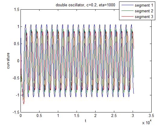
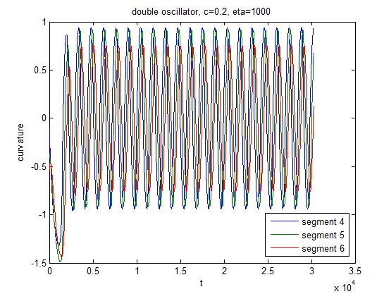
21 when c=0.5, which is too large for the wave to propagate when there is only one oscillator. The phase difference between segments, seems to be insensitive to c. This coincide with the case of one single oscillator. Other parameters: η = 1000, k=0.5. As an example, we simulate the detailed dynamics when c=0. and η = 1000.

22

23 We also simulate the case that the head is repressed by blocking the stimulation from y(4) to y(5), and from y(6) to y(7). This means the muscle of segment and segment 3 cannot provide any torque at all. In this case we find that the rear part of the worm oscillate in an independent and fast frequency. Since all the head oscillator can dominate over the middle oscillator, we do not need to develop a new analytical explanation especially for worms containing two oscillators. The basic mechanism behind all these phenomenon can be attributed to forced oscillation, which is only a simple physical concept. Attempt to introduce gap junction to oscillators We have not introduced any gap junction to oscillators so far. This is because that excessively strong gap junction could be detrimental to the oscillators. However, this is not very reasonable because it is observed in the experiments that when the middle part of the worm is repressed, the head will also be still, which indicates that the motion in the middle can affect the motion of the head. Since proprioception can only propagate wave form head to the tail, it must be gap junctions that affect the head oscillator. Here we fix c=0. and η = 1000, and we vary the strength of the gap junction linked to the oscillators, which we denote as c 1 below, to see how we should solve this problem in the model. As an attempt, we first allow the gap junction to be not balanced, which means the two segments can influence each other in different extent, but with the same gap junction. This is still not very reasonable, we may modify this later. We find that the maximal strength of the gap junction is about Beyond this value, the whole worm will paralyze. Within the small regime from 0 to 0.04, the minimal

24 amplitude is increasing. We also find that the frequency decreases as c 1 increases. Theoretically, after introducing gap junctions to the oscillators, the mid-oscillator can affect and adjust the frequency of the head oscillator. However, we have not found this phenomenon. On the contrary, the frequency of the mid oscillator is always determined by head. This may be because introduced gap junction is much weaker then proprioception. Then we change the assumption of the gap junction. We stipulate that the mutual influence via gap junction is equal for both adjacent segments. We find that the strength here, denoted as c, has similar effect on the network as c 1. Since the proprioceptive coupling is already sufficiently strong, weak gap junction of

25 oscillators will not lead to severe attenuation. So this can be a good way of incorporate gap junction into the oscillators in our model.

26 There can be another way to understand the dynamics of the oscillators. We can postulate that the intrinsic dynamics of oscillator is very robust, which can be hardly affected by the gap junctions. We can write the dynamic equation in the form: (Mτ) dv dt = M(f(v) + g(u)) + c(v i 1 + v i+1 ). M can be seen as the robustness of the intrinsic dynamics of the oscillator. If M > 1, c can also be larger, and approximate the c of other segments.