Infrared Spectra of Protonated Networks of Water Molecules in the Interior of Bacteriorhodopsin: A QM/MM Molecular Dynamics Study. Volker Kleinschmidt

Transcription

1 Infrared Spectra of Protonated Networks of Water Molecules in the Interior of Bacteriorhodopsin: A QM/MM Molecular Dynamics Study Volker Kleinschmidt Bochum, 2006

2

3 Infrared Spectra of Protonated Networks of Water Molecules in the Interior of Bacteriorhodopsin: A QM/MM Molecular Dynamics Study Dissertation am Lehrstuhl für Theoretische Chemie der Ruhr-Universität-Bochum vorgelegt von Volker Kleinschmidt geb. in Bremerhaven Bochum, Januar 2006

4 Erstgutachter: Prof. Dr. Dominik Marx Zweitgutachter: Prof. Dr. Volker Staemmler Tag der mündlichen Prüfung:

5 Abstract This work tries to computationally provide some evidence for the presence of one (or more) protonated networks of water molecules inside of the protein bacteriorhodopsin (BR), and thereby proving the importance of these single water molecules in the proton-translocation process of this light-driven molecular machine. For that purpose, a BR system on the molecular level comprising the 7 α helix transmembrane BR protein monomer, the embedding cell membrane, and a surrounding aqueous medium was constructed and subsequently equilibrated. As the site for that hypothetical protonated water cluster within the BR protein, a cavity near the extracellular side of the proton-pumping channel has been chosen (bounded to the extracellular side by the glutamate 194/204 pair of amino acids). Before starting with a quantum-mechanical / molecular-mechanical (QM/MM) dynamical simulation in order to calculate the infrared (IR) spectrum of two different topologies of protonated water clusters, embedded in the BR protein environment, the used GROMOS/CPMD interfacing program has first been validated on grounds of test calculations on smaller aqueous molecular systems (protonated and unprotonated). It was shown that the interface slightly overestimates the intermolecular forces between the QM and MM parts in those examples, due to a static bulk-water parametrization of the MM water molecules, which yields an increased molecular dipole moment. For the case of a proton-sharing, solvated Zundel (H 5 O H 2 O) topology embedded in the above-mentioned cavity, an excellent agreement in the range of 1800 to 2100 cm 1 could be identified between the computed Zundel s continuum band and a measured Fourier-transform IR spectrum (being a difference spectrum between the BR ground-state and its M respectively N intermediate structure). For the case of a star-like Eigen (H 3 O + 3 H 2 O) topology, instead, embedded in the same cavity, the general shape of the pronounced Eigen peak could be recovered in an experimental BR groundstate minus K/L-intermediate difference IR spectrum, but shifted with respect to the computed IR spectrum inside of BR by about 600 cm 1. Further conclusions, related to the question of what kind of protonated water clusters are located at which site in the BR channel and during which period of the BR proton-pumping cycle that can de facto be drawn from these findings, are also discussed in molecular detail, highlighting both, theoretical and experimental limitations and uncertainties.

6

7 Contents List of Figures List of Tables v vii 1 Introduction and Biological Background 1 2 Bacteriorhodopsin: Structure and Functionality Discussion of the BR Photocycle Crystallographic Diffraction Methods for BR The BR Ground-State The K-Intermediate The L-Intermediate The M-Intermediate The N-Intermediate The O-Intermediate IR Spectroscopy on BR / Motivation for this Work Infrared Spectroscopy Broad IR Absorption Bands of Protonated Water Clusters Molecular Dynamics Methods Classical Force Fields Potential Forms Force Calculation and Boundary Conditions MD Integration and Extensions Car Parrinello Molecular Dynamics Basic Equations and Thermostatting Density Functional Theory and Pseudopotentials The QM/MM Interface Program Organization and Keyword Specification Interactions between QM and MM Part i

8 Contents 4 System Set-up and Equilibration Single Components of the System The Protein The Membrane The Water Layer Force Field Parametrization The Lysine Retinal Residue The Zundel Cation The POPC Phosphorlipid The Course of Equilibration Relaxation and Equilibration under CHARMM Further Phases of Equilibration under GROMOS Structural Changes During the Equilibration Structure and Stability of the Biomatrix Preparations for the QM/MM Run Infrared Spectroscopy: Some Theoretical Background Information IR Spectra from MD Trajectories Normal Mode Analysis Calculation of the Electronic Dipole Moment Some Practical Computational Issues Rotational Corrections Autocorrelation Functions Discrete Fourier Transformation Dipole Decomposition Techniques Test and Reference Calculations in the Gas Phase IR Spectra of Protonated Water Clusters QM/MM Calculations The Water Dimer The Solvated Hydronium (Eigen Cation) The Zundel Spectrum Investigated by Dipole Decomposition IR Spectra of Protonated Waters Clusters in BR Electrostatics of the Glu194 /Glu204 Pocket The embedded Eigen Cation The embedded Zundel Cation Comparison with Experiments Discussion and Future Perspectives 159 ii

9 Contents A Force Field Parameterization: Some Supplemental Information 167 A.1 The Lysine Retinal Residue A.2 The Zundel Cation A.3 The POPC Phosphorlipid B Amino Acid Abbreviations 173 Bibliography 175 iii

10

11 List of Figures 1.1 The Halobacterium on Different Length Scales The BR Channel in Top-View Perspective Different Steps of Proton Translocation within BR The BR Photocycle Different Conformations of the Chromophore in the Gas Phase Location of Channel-Internal Water Molecules (Standard Orientation) Location of Channel-Internal Water Molecules (Pentagon Structure) Conformation of the Chromophore in the K-State Sketch of the Grotthuss Mechanism Measured Intermediate Minus Groundstate FTIR Spectra QM Box Embedded in a Large Molecular-Mechanical System Total BR System after Equilibration A Monomer of the POPC Phosphorlipid Various Stages of Membrane Preparation Total BR System before Equilibration Energy, Pressure and Volume during Equilibration under CHARMM Energy and Temperature during Equilibration under GROMOS Pressure and Volume during Equilibration under GROMOS Atomic Root-Mean-Square Deviations during Equilibration Structural Changes within BR during Equilibration under CHARMM Structural Changes within BR during Equilibration under GROMOS Structural Changes within BR during Overall Equilibration Time Density Profile of Different Components of the BR System Orientation of the POPC Monomers within the Membrane as Characterized by the Order Parameter Sk CC Dipole Rotational Corrections as Applied to the H 2 O Molecule Illustration of a Discrete Fourier-Transformation The Three Normal Modes of H 2 O The Six Normal Modes of H 3 O IR and Stick Spectra of Various Protonated Water Clusters Selected Normal Modes of H 5 O + 2 (The Zundel Cation) Selected Normal Modes of H 7 O Selected Normal Modes of H 9 O + 4 (The Eigen Cation) v

12 List of Figures 6.7 IR and Stick Spectrum of H 5 O H 2 O Selected Normal Modes of H 5 O H 2 O Ball-and-Stick Model of a QM/MM Water Dimer QM/MM vs. all-qm Water Dimer: O O Distance Distribution QM/MM vs. all-qm Water Dimer: Dipole Distribution of the QM H 2 O QM/MM vs. all-qm Water Dimer: IR Spectrum of the QM H 2 O Ball-and-Stick Model of a QM/MM Eigen Cation QM/MM vs. all-qm Eigen Cation: Distance and Angle Distributions QM/MM vs. all-qm Eigen Cation: Dipole Distribution of the QM H 3 O QM/MM vs. all-qm Eigen Cation: IR Spectrum of the QM H 3 O The Zundel Cation: Experimental vs. Computed Gas-Phase IR Spectrum The Zundel Cation: Decomp. of the IR Spectrum into Core and Ligand Part The Core-Zundel Part: Decomp. of the IR Spectrum in Parts and to the O O Axis The Core-Zundel Part: Further Decompositions of the Spectral Part The Zundel Cation: Characterization of the Geometry The Zundel Cation: MD Trajectory Flipping Events The Zundel Cation: Sketch of a Flipping Event The Zundel Cation: Sketch of Two Lowest Energy Conformations The Zundel Cation: Torsional Angle Dynamics around the O O Axis Electrostatics of the Glu194/Glu204 Pocket The Eigen Cation as Embedded in the Glu194/Glu204 Pocket IR Spectrum of the Eigen Cation: Gas Phase vs. Embedded in BR Hydrogen Bond Dynamics in the Glu194/Glu204 Pocket (1) Hydrogen Bond Dynamics in the Glu194/Glu204 Pocket (2) The Solvated Zundel Complex as Embedded in the Glu194/Glu204 Pocket Solvated Zundel IR Spectrum: Gas Phase vs. Embedded in BR Eigen- vs. Solvated-Zundel IR Spectrum in BR Eigen- vs. Solvated-Zundel IR Spectrum in BR: Continuous Superposition Measured vs. Computed IR Spectra in BR Sketch of the Pentagon Structure below the Schiff Base A.1 Chemical Structure of the Retinal Lysine Complex A.2 Chemical Structure of the Zundel Cation vi

13 List of Tables 2.1 A Selection of BR Molecular Structures from the Protein Data Bank Size of the BR System in Terms of Number of Residues and Atoms A.1 The Lyr Residue: CHARMM and GROMOS Atomic Partial Charges A.2 The Lyr Residue: Force-Field Constants of, and Energy Barriers around Selected Bonds A.3 The Lyr Residue: Comparison between Experimental, DFT and Force- Field Predictions for Selected Bond Lengths A.4 The Zundel Residue: GROMOS and CHARMM Force Field Parameters vii

14

15 1 Introduction and Biological Background This work is about computational studies on bacteriorhodopsin (BR). BR, as a protein in the cell membrane of the archaebacterium 1 halobacterium salinarum, 2 has been first discovered by Oesterhelt and Stoeckenius [1], in Halobacterium salinarum, in turn, is a prokaryotes of rod-like form with a length-size of about 5 µm, being also equipped with a flagellum that enables it to change position in an aqueous medium (see Fig. 1.1 (b)). Halobacterium salinarum furthermore is strongly halophilic, meaning that it finds ideal living conditions in extreme NaCl-rich aqueous environments, like salt ponds or salines, for instance, which then often show up a characteristic deep purple coloring (an example is shown in Fig. 1.1 (a)). Concerning power supply, halobacterium salinarum is facultative anaerobic, implying that in oxygen-poor environments it can resort to energy sources other than the physiological degradation of organic food substances. The very unique property of the bacteriorhodopsin protein being strongly enriched in the cell membrane of halobacterium salinarum in case that not sufficient O 2 is available then constitutes the energy alternative for this archaebacterium. In fact, BR has the ability of directly converting sun-light energy into an electrochemical H + gradient across the cell membrane, which then further is exploited by the archaebacterium for ATP production (more details are given below). The way of how the BR protein accomplishes for this task, can be directly guessed from its molecular structure. From X-ray crystallographic measurements it is known that the 248 amino acids, the BR polypeptide is composed of, fold themselves basically into 7 α helices that span the cell membrane in vertical direction, and thereby form the surroundings of a channel-like structure (see Fig. 2.2 for a BR monomer, and Fig. 1.1 (d) for the trimer case), in the interior of which the protons are transported from the cytoplasmatic side of the cell to the extracellular medium. Some of the inward reaching side chains of the protein, of course, play an active role in this H + conduction process by functioning as interstitial proton storage sites. 1 Cell biologists subdivide living cells into two principle categories: the prokaryotes which are more primitive in structure, neither having a separated DNA-containing nucleus, nor other selfcontained cell organelles; and the more developed eukaryotes which feature these kind of compartmentation. The prokaryotes are further classified into real bacteria (sometimes also termed eubacteria) and archaebacteria (or simply archae). 2 The terminology for that archaebacterium somewhat varies in literature; alternative names, frequently encountered, are e.g.: halobacterium salinarium, halobacterium halobium or halobacter halobium. 1

16 1 Introduction and Biological Background (a) (b) ~5 µm (c) (d) 10 nm 2 nm Figure 1.1: (a) Salt crystallization basins with blooming populations of halobacteria, which color the water deeply purple. (b) Single archaebacteria of type halobacterium salinarum, recorded by electron microscopy. (c) Atomic force microscopic photo of the cell membrane of halobacterium salinarum from the cytoplasmatic side [2], showing the single BR trimers approximately arranged in a 2-dimensional hexagonal lattice. (d) Picture of a BR trimer in ribbon representation ; protein structure taken from the 1BRR entry [3] out of the Protein Data Bank [4]. But the most important part in this respect is attributed to the central retinal chromophore (also shown in Fig. 2.2, as well as in Fig. 2.4), since it is that part of the BR protein which provides the amount of energy necessary to make possible the transport against an existing H + gradient across the cell membrane. The photoinduced all-trans to 13-cis isomerization of the retinal s unsaturated hydrocarbon chain (see Fig. 2.4) promotes the directional H + transfer in a twofold manner: on the one hand, this isomerization provides a loosely bond proton at the retinal s Schiff base (N H group) in direct neighborhood to the isomerization center; and on the other hand, due to the hindered nature of the conformational changes after isomerization, the photoexcited retinal exerts some significant tension on its molecular environment especially on the helix to which the chromophore is covalently bond to by a lysine bridge; these structural disturbances than further propagate into the protein where they initiate the global structural changes on a molecular level that makes possible the net transport of one H + per single photoexcitation event. 2

17 This so-called BR photocycle discussed in some detail in the next chapter altogether involves a couple of five different H + translocation steps along the 7 α helix channel, which, in combination with some steps of structural relaxation towards the end of the cycle, lead back the BR protein inclusively its retinal chromophore into its initial state (from where it is, of course, again photo-excitable). In this manner a single BR trimer is capable of pumping a few hundred protons per second across the cell membrane of halobacterium salinarum. Having arrived at the extracellular side, the protons are directly conducted along the surface of the cell membrane to the ATP synthesis center of the archaebacterium the so-called ATP synthase. This enzyme is a likewise transmembrane (but not a 7 α helix) protein that is driven in the phosphorylation of ADP to ATP by the electromotive force of the back-flowing H + ions into the cytoplasm. [Only as a side remark it is mentioned here that higher eukaryotic organism, like the cells of the human body for instance, also accumulate their ATP energy reservoir by means of the ATP synthase enzyme; in opposite to BR however, the necessary H + gradient (across the inner membrane of the mitochondrion, in that case) is not build up by direct energy conversion from sun light, but in the framework of the so-called respiration chain, which is the final step in the metabolism of energy-rich food substances, like e.g. glucose or triglycerides, to CO 2 and H 2 O under the consumption of O 2 ; see any textbook about biochemistry.] Bacteriorhodopsin is not the only retinal protein with a special physiological task in halobacterium salinarum. There is also the anion pump halorhodopsin (HR) [5] [3], which pumps, initiated through the photoexcitation of the retinal subunit, Cl anions in opposite the direction as BR pumps H + cations that is, from outside of the cell to the inside. HR is very similar in structure to BR, but occurs in the cell membrane of halobacterium salinarum only with 5 10 % of the abundance of BR. Its physiological purpose is not to gain energy, but to regulate the cell s ion household. Moreover the cell membrane of halobacterium salinarum also hosts the two different sensory rhodopsin complexes, SRI and SRII [6] [7], which enable the bacterium to react by phototaxis on changes in intensity and spectral composition of the incoming radiation. Of course, terms like retinal and rhodopsin are first of all associated with the viewing process of higher organism. In fact, the light-sensitive rhodopsin protein, that can be found in high quantities in the viewing cells (so-called rods and cones) of the retina of our eyes, also is a transmembrane 7 α helix protein with a central retinal chromophore. Despite of the structural similarity between visual rhodopsin (VR) and bacteriorhodopsin, their respective photocycles differ in many respects. One point is, that the photoisomerization of the retinal in VR happens from 11-cis, as the ground-state form, to all-trans, as the excited-state form (in BR its from all-trans to 13-cis). Another striking difference as compared to the BR cycle is that in course of the conformational changes of visual rhodopsin after photoexcitation, 3

18 1 Introduction and Biological Background the retinal chromophore is spatially separated from the protein residue (called opsin then) by hydrolytic bond splitting; making both, a reisomerization of the retinal and a reunification of it to the opsin necessary for ground-state recovery. In the photocycle of visual rhodopsin a directional H + translocation occurs as well; but this kind of charge separation does not represent the neural signal that is arisen by a hitting photon onto the retina. It is known that a single rhodopsin protein in the excited-state conformation, instead, puts into operation a cascade of self-enhancing signal processes in the cytoplasm that finally result in the closing of some hundred cation-specific membrane channels which otherwise would stay opened in the dark-state of the viewing cells. By this light-induced ion-channel closing, as strong hyperpolarization along the cell membrane of the rods (or cones) is generated, constituting the neural signal that further is conducted to the brain. [A fairly good description of the viewing process is given in [8], for instance.] The functionality of rhodopsin in the framework of the viewing process is just one example from the large class of so-called G-protein-coupled signal receptors. Characteristic for this receptor family is their transmembrane 7 α helix structure, embedding a central active molecular unit. The active unit of these proteins can either be receptive to light signals (as in the case of VR), or else, can work as docking site for external message molecules; like, for instance, a molecule of scent in the process of smelling, or body-own substances like hormones that are transported with the bloodstream to the receptor. In its signal-excited form, a 7 α helix protein then usually couples to a transmitter G-protein on the cytoplasmatic side of the cell membrane, which in turn puts into operation the suitable enzymatic reaction inside the cell, as response to the external stimulus (see e.g. [8] for more detailed informations). The just mentioned examples from biochemistry should have made clear that the class of 7 α helix proteins plays a key role in the process of signal transduction in the human body. Thus, there exists a strong interest in the functionality of these receptor proteins from the side of medical drug design, for instance. But in the past, it has been difficult to accumulate, purify or even crystallize such proteins, necessary for structural investigations. For BR instead, which naturally occurs in a regular 2-dimensional arrangement in the cell membrane of halobacterium salinarum (as shown in Fig. 1.1 (c)), crystallization was easier to accomplish; consequently, BR was serving for some time as the only prototype for a 7 α helix receptor protein making understandable the large scientific interest in this specific molecular system from that perspective. The BR system is of course also of interest in its own right, since one could imagine to employ the sun-light converting capability of that protein for biotechnological energy production purposes, or, on a less large scale, for applications in optoelectronic devices. 4

19 Today BR constitutes one of the best understood biomolecular machines, whose functionality has been discovered to a very large extent; except for some details on the atomistic level that still are left open for explanation. The precise conformational changes of the retinal chromophore after the photoexcitation, for instance, are not yet fully resolved (respectively, there exists controversial measurement results on this issue; as discussed in Chap. 2). Likewise, not all of the channel-internal H + translocation pathways, respectively, the H + storage sites along the BR channel have fully been identified so far. Although two important key aspartate amino acids (Asp85 and Asp96, see Chap. 2) could be identified, whose COO carboxyl acid residue takes up a H + at different stages of the BR cycle, respectively, it is, for instance, still unclear from which molecular group of the BR protein the proton is finally released into the extracellular medium (this group is usually termed as proton release group). In recent years, the idea came up that a network of channel-internal H 2 O molecules also could participate in the H + conduction and storage processes; particularly since the existence of such networks within BR now is proven experimentally due to the improved resolution in X-ray spectroscopy. Additionally, there are hints from IR spectroscopy on broad absorptional bands (extending over a few 100 wavenumbers) during some stages of the BR cycle, as these are characteristic for the IR spectrum of the different species of protonated H 2 O clusters (see Chap. 6). The scientific aim of this work now is to probe the hypothesis of protonated water clusters inside of BR by simulation methods. For that purpose, we have placed two suitable, simply protonated clusters composed out of 4, respectively, 6 water molecules in a larger cavity near the extracellular exit of the BR channel (where a similar number of water molecules also is seen by X-ray spectroscopy), in order to compute their respective IR spectra by employing a combined quantum-mechanical / molecular-mechanical (QM/MM) dynamical approach. Especially with respect to the broad absorptional bands (those which are indicative for the protonation of the water clusters), the compute spectra are then compared to the experimental ones that have been recorded by (time-dependent) Fast Fouriertransform Infrared Spectroscopy (FTIR) on BR. Although this task might, at first, not sound very complicate, many preparatory steps have however been necessary in order to make these calculations possible. First of all, it essential to understand the single steps in the BR cycle, as well as the way of how the experimental FTIR spectra are recorded during that cycle. This understanding is required in order to be able to select the right intermediate BR structure for the calculation (there are different such structures according to the conformational stage of the BR protein during the photocycle, see Chap. 2), and therewith in connection, to develop a judgment of how far the comparison between computed and measured spectra can be drawn. 5

20 1 Introduction and Biological Background These issues are dealt with in Chapter 2. In Chapter 3, a review is given about the QM/MM molecular dynamical methods used for our simulations. Chapter 4 describes the way of how the overall simulated BR system comprising the BR protein itself, a cell membrane build-up from double-layered phosphorlipid monomers, as well as two (top and bottom) covering water layers has been set up and, that followed, stepwise equilibrated. Chapter 5 again is a methodic chapter, providing some theoretical and also practical background information on the methods we have used for computing the IR spectra. Chapter 6 then shows the results of some QM/MM test and reference calculations of various (mainly protonated) water clusters, among them also those two species whose IR spectra later on were calculated inside of BR; while in Chapter 7 these two IR spectra inside of BR are finally presented, and discussed with respect to their experimental counterpart spectra. The Chapters 4 and 6 describe in detail the content of our publication [9], while the same is true for Chapter 7 with respect to our second publication [10]. 6

21 2 Bacteriorhodopsin: Structure and Functionality 2.1 Discussion of the BR Photocycle In this section we want to take a closer look to the interconnection between structural changes in BR on the molecular level and the single steps involved in its physiological task as a proton pump. On grounds of light absorption measurements, the overall proton pumping cycle has historically [11] been subdivided into the unexcited ground state (BR) and a sequence of, at least, 5 excited intermediate states denoted in Fig. 2.3 by capital letters from K to M. During the course of one pumping act these intermediates sequentially convert into each other with different lifetimes in between them. Each of these substates is experimentally identified by a different wavelength (in nm) where maximal light absorption of the retinal chromophore within BR takes place (seen in Fig 2.3 as subscripts at the symbol for the intermediates). Another way of characterizing the pumping cycle is in terms of key proton translocation steps. After a period of more than 30 years of intense research on BR, it seems to be established now, that the pumping act (also) involves five principle H + translocation steps (which not directly correspond to the five spectroscopically characterized intermediate states). Figure 2.2 sketches these 5 steps as they are embedded in the 7 α helix protein structure; also shown are the retinal/lys216 complex and the key amino acids Asp96, Asp85, Arg82, Glu194 and Glu Together with the photoisomerization of the chromophore and its re-isomerization at a later stage, the BR cycle thus can be summarized as follows (compare with Fig. 2.2): Retinal isomerization: The BR cycle starts with the photoisomerization of the retinal from the all-trans to the 13-cis conformation (BR K transition in Fig.2.3). Step 1: Roughly 1 µs after the photoexcitation a proton dissociates from the positively charged Schiff base (N H + group) of the excited retinal, being taken-up by the negatively charged carbonyl group of Asp85. 1 For the nomenclature of amino acid abbreviations see Appendix B. 7

22 2 Bacteriorhodopsin: Structure and Functionality Step 2: The protonation of Asp85 in the previous step establishes the conditions for the release of one proton from the so-called proton release group (PRG) into the extracellular medium during the late M-intermediate. Step 3: The next principle step in the photocycle, which also marks the M N transition in the spectroscopic classification, is the reprotonation of the deprotonated Schiff base from the cytoplasmatic side with Asp96 acting as a proton donor. Step 4: In the late N-intermediate (sometimes also termed as N ), the reprotonation of Asp96 from the intracellular side takes place. Retinal re-isomerization: A thermally driven back-isomerization of the retinal into the all-trans conformation happens during the O-stage of the photocycle. Step 5: Finally, the initial state of the photocycle is reestablished when the Asp85 carboxyl group is deprotonated back again. Further details and certainly still open questions in the functional process of the photocycle will be discussed in more detail when we take a closer look to the various atomic structures being available for BR in the ground state and for its intermediates. But before doing so, we should give a small account on those methods, which are nowadays actually used to clarify the atomic structure of proteins, in general, and that of BR in particular. Asp85 B C Glu194 D A Schiff base + Retinal G Asp96 Glu204 F E Figure 2.1: The same BR structure as in Fig. 2.2, but shown here in a top-view perspective, that is, when looking from the cytoplasmatic side onto the BR monomer. The capital letters from A to G denote the 7 α helices as in Fig

23 2.1 Discussion of the BR Photocycle Cytoplasmatic Side Step 4 A G B Step 3 F Asp96 C E D Lys216 Step 1 Schiff base Retinal Step 5 Asp85 Glu204 Step 2 Glu194 Extracellular Side Figure 2.2: BR monomer in the ribbon representation (the 7 α helices are labeled from A to G). Shown are the five principle H + -translocation steps of the BR photocycle together with the Lys216+Retinal chromophore-complex (hosting the Schiff base in between them) and some of the key amino acid residues. [Step 1 to step 5 are briefly summarized on pp. 7.] 9

24 2 Bacteriorhodopsin: Structure and Functionality Figure 2.3: The photocycle of bacteriorhodopsin. Intermediate states are denoted by capital letters from K to O; br here stands for the BR ground state. The subscript numbers at these letters relate to the absorption maxima (in nm) for the different BR states. Also specified are approximate lifetimes of the different intermediates. all trans, 15 anti CH 3 CH 3 CH CH 3 Η 15 lysine bridge ε γ + δ N Schiff base Η β back Η α bone CH 3 β ionine ring 13 cis, 15 sys CH 3 CH 3 CH CH 3 CH 3 Η 15 + N ε δ γ β α Η Η 13 cis, 15 anti CH 3 CH 3 CH CH 3 CH 3 Η 15 + N ε δ H γ β α Η Figure 2.4: Chemical structure formulae showing the BR retinal+lysine complex in three possible conformations (whereby the final two are excited-state ones). 10

25 2.1.1 Crystallographic Diffraction Methods for BR One way to gain structural information about proteins is by diffraction techniques. This requires first to crystallize the protein sample as perfect as possible, and then to radiate it either by X-rays, electrons or neutrons. 2 In this way, a 2-dimensional diffraction pattern is generated, whose Fourier transform gives a direct picture about the electronic density in the protein. For the purpose of protein structure determination, illumination by X-rays usually gives the highest resolution; using a novel crystallization technique, where the crystals are grown in a so-called lipidic cubic phase (LQP) [13, 14], for BR, a resolution higher than 1.5 Å has been reached; whereas when employing electron diffraction on a crystal of the same quality one usually cannot do better than about 3.5 Å of resolution (see Tab. 2.1). 3 Next to the growing of most perfect protein crystals, another problem, which arises when one wants to apply X-ray crystallography to the intermediates of BR, lies in trapping and conserving these intermediates. For the intermediates at the beginning of the photocycle (K, L, early M) the trapping usually is done by illuminating the (crystalline) BR sample by red or green laser light for a specific period of time at lower than ambient temperatures; subsequently, after a certain period of rest, the protein is than shock-frozen for conservation. The choice of the specific wavelength of light by which the chromophore inside the BR is excited, the temperature under which this is performed and the duration of the resting-time before freezing, are all parts of a specific trapping protocol [16] and depend on which of the intermediates one wishes to accumulate in the protein sample. For the intermediates in the second half of the photocycle (late M to O) the sole trapping-by-illumination method in general no more is practicable, and one usually resorts to the strategy to use specific mutants, slowing down the decay of the desired intermediate. As an example, the D96N mutant, which strongly prevents the Schiff base from being reprotonated from the cytoplasmatic side, is used to highly populate the late M-intermediate. However, it should be kept in mind that a mutated species, of course, is at least locally no more identical to the wild-type intermediate. Table 2.1 shows a selection of BR ground-state and intermediate structures, recently recorded by either X-ray or electron crystallography. 2 Neutron diffraction experiments gave the first hints upon the presence of H 2 O molecules inside of the BR proton-pumping channel [12]. 3 Many useful background informations on X-ray crystallography for proteins are given in the book [15], which might be helpful, among other things, in judging the quality of a reported X-ray protein structures. 11

26 Table 2.1: Selected BR ground-state and intermediate structures from the Protein Data Bank (PDB) [4]. Species a Trapping Cond. b Occupancy [%] Resolution, [Å] PDB File Ref. BR (wild-type) no illumination C3W [17] BR (wild-type) no illumination QHJ [18] K (wild-type) green light, 110 K QKP [19] K (wild-type) green light, 100 K M0K [20] L (wild-type) green light, 170 K E0P [21] L (wild-type) red light, 170 K O0A [22] L (wild-type) green light, 170 K followed by red light, 100 K UCQ [23] M1(wild-type) red light, 210 K M0M [24] M1(wild-type) yellow light, 230 K KG8 [25] M1(wild-type) red light, 295 K P8H [26] M2(E204Q) red light, 295 K > F4Z [27] M2 (D96N) red light, 295 K C8S [17] M2(wild-type) green light, 295 K CWQ [28] late M and N no illumination, (D96G/F171C/F219L) e in plane 1FBK [29] crystallography 3.60 vertical N (V49A) red light, 295 K P8U [26] O (D85S) no illumination JV7 [30] a For the nomenclature of amino acid abbreviations see App. B. b If not otherwise stated X-ray crystallography was used. 12

27 Asp Lys Schiff base Asp212 Asp Retinal Arg82 Glu Glu194 Figure 2.5: Locations of channel-internal water molecules (whose oxygen atoms are marked by red balls) inside of the Luecke ground-state structure 1C3W (compare with Tab. 2.1). Asp Lys Asp85 Schiff base 402 Asp Arg Retinal Glu204 Glu194 Figure 2.6: Same as in Fig. 2.5, but orientated in such a way that the pentagonal arrangement between Wat402, Asp85, Wat401, Wat406 and Asp212 clearly is recognizable. 13

28 2 Bacteriorhodopsin: Structure and Functionality The BR Ground-State Mainly due to the long temporal stability, BR is best know in its ground-state structure, as compared to the various intermediate states whose structural identification most often is hampered by serious trapping, respectively, mixing problems. Next to the two explicit ground-state structures listed in Tab. 2.1, ground-state structures usually are specified as well as a by-product in the structural investigation of any of the intermediate states. Provided that their spatial resolution is sufficiently high, the reported groundstate structures usually show the retinal in the planar all-trans conformation. The retinal/lys216 composite residue separates the channel region in a cytoplasmatic (upper) part and an extracellular (lower) part (see Fig. 2.2). There is general agreement in all recent (highly resolved) ground-state structures that the cytoplasmatic half only contains a few channel-internal water molecules (2 3 ones), while the extracellular part of the channel has 7 8 of them (as shown in Figs. 2.5 and 2.6). From the later ones, 3 are arranged together with the Schiff base and the two negatively charged carbonyl groups of Asp96 and Asp212 into a stable hydrogen-bonded pentagon topology; the forth water molecule resides near the positively charged guanidinium (C 2(NH 2 )) group of Arg82; and finally the 3 4 remaining ones are clustered in a second hydrophilic pocket on the extracellular side of the channel, which is upper-bounded by Arg82, respectively lower-bounded by the two glutamates 194 and 204. [Fluctuations in the number of channel-internal water molecules on the nanosecond scale have been investigated in [31, 32] on the level of classical (force-field) molecular dynamics.] The K-Intermediate The K-intermediate reflects the changes in the BR structure directly after the photoexcitation; 4 these changes, of course, are primary restricted to the retinal and to the Lys216 residue, which covalently bridges the retinal to the protein backbone. It is generally accepted now that the C 13 =C 14 double bond is photoisomerized from the trans to the cis form. For a retinal lysine complex in free solution for example, this kind of isomerization would imply a large-scale bending motion of both ends of the molecule around the C 13 =C 14 bond (this bending effect is most pronounced in the 13-cis, 15-anti conformation, see Fig. 2.4). But not so for the case of BR, where both ends of the retinal lysine complex are rigidly embedded in the protein environment (by hydrogen bonds around the ring-terminated side and by a covalent bond on the opposite side). 4 The excitation process as such, respectively, the dynamics in the excited state, is not discussed at this point; but see footnote 9 on p. 21 or the discussion in the summary starting on p

29 2.1 Discussion of the BR Photocycle Lyr216 Schiff base Nitrogen N C 14 C 13 C ε C A Retinal Wat402 Figure 2.7: Conformational changes of the retinal+lysine chromophore inside of BR after photoexcitation (to be compared with Fig. 2.4). Gray structure: all-trans, 15-anti conformation of the chromophore in the BR ground-state (from the PDB entry 1M0L [20]). Colored structure: distorted 13-cis, 15-anti conformation, as X-ray measured in the K-state (from the PDB entry 1M0K [20]). The only way out of this conflict then is a local twisting motion around bonds in the vicinity of the C 13 =C 14 isomerization center; namely around the C 14 C 15, C 15 =N and N C ɛ bonds in direction to the lysine (see Fig. 2.4). The crucial point now is: will the Schiff base N H group still point to the extracellular (downward pointing) side after the photoisomerization, or will it have swapped towards the opposite direction, breaking the hydrogen bond to Wat402 present in the ground state? According to the (planar) structure formulae of the retinal/lysine complex in Fig. 2.4, the former case would be true in the 13-cis, 15-anti conformation, while the latter case is realized in 13-cis, 15-syn. Unfortunately, the local conformation of the atomic chain, say, between C 13 and C ɛ is only hard to resolve by X-ray diffraction; thus already early infrared and Raman investigations [33, 34, 35] have been performed on exactly this issue, with the result that in the K-state the retinal is supposed to be in the twisted 13-cis, 15-anti conformation. More recently, an effort has been undertaken to determine this retinal conformation of interest by a highly resolved (1.43 Å) X-ray study [20]. The resulting structure (see Fig. 2.7) shows, as suggested by the infrared and Raman studies, a (rather distorted) 13-cis, 15-anti conformation of the retinal, whose strong local twisting enables the Schiff base to still approximately direct to the extracellular side (in contrast to the non-twisted 13-cis, 15-anti structure in Fig. 2.4). In that case, the hydrogen bonding to water 402 is rather distorted, as well, exhibiting an unfavorable N H O angle of 116 ±

30 2 Bacteriorhodopsin: Structure and Functionality On the other hand, a second, earlier X-ray structure for the K-intermediate exists [19] as well. But in this work, during the process of crystallographic refinement, the retinal conformation was a priori constrained to the relaxed 13-cis, 15-anti case, with the Schiff base directing to the (upper) cytoplasmatic side (in contrast to the afore mentioned K-structure) The L-Intermediate The L-intermediate is the stage in the photocycle where the system prepares for the H + -transfer from the Schiff base to the Asp85 during a time interval of 1 µs. At the time of writing this thesis, three rather different structures for the L-intermediate were available (see Tab. 2.1). The furthermost back-dating L-structure [21] (which has been reconfirmed in a more recent work [36]) shows a large-scale motion of the helix C in direction to the interior of the channel, and, as a result, an approaching of Asp85 (which is a part of helix C) towards the Schiff base. This large-scale motion of helix C is driven by a continuing dissolvation of the hydrogen bonded water side-chain network on the extracellular half of the channel; which, in turn, already started in the preceding K-state structure [19], and should thus have been initiated directly by the photoisomerization of the retinal. In contrast to these findings, the second paper on the L-intermediate [22] does not report any large-scale motions on the extracellular side at all; but alternatively some minor rearrangements of groups on the cytoplasmatic side. More importantly, this group has dedicated some considerable effort like in their study of the K-state [20] to X-ray resolve the local conformation of the retinal during L; their finding was that the retinal switches from a distorted 13-cis, 15-anti (in K) to 13-cis, 15-syn conformation (in L), simultaneously re-straightening the hydrogen bond between the Schiff base and the (still) nearby Wat402. The most recent structure on the L-intermediate [23] finally, sees the retinal in a non-twisted 13-cis, 15-anti conformation with the Schiff base pointing to the cytoplasmatic side. Moreover, the water molecule directly below the Schiff base in the ground state has been disappeared in this L structure; on the other hand, a new water, not present in the ground state, now shows up on the cytoplasmatic side directly on top of the flipped Schiff base. This observation strongly suggest that, in the K-to-L transition, a water molecule takes part in the 180 rotation of the Schiff base and thus being dragged by hydrogen bonding forces from the downward side of the retinal to its upward side. Further structural differences in this reported L-intermediate [23], as compared to the ground state, are mainly confined to the cytoplasmatic side of the channel in the region directly above the retinal; there, a bucking motion of the retinal s hydrocarbon chain cause a upward movement of the C 13 -methyl group, whereby, in turn, some close-by groups (Leu93, Trp182 and Wat601) are pushed aside. 16

31 2.1 Discussion of the BR Photocycle Recapitulating, one is led to the suspicion that, due to the really grave differences in the three L-structures introduced here, there must exist serious hidden problems in either trapping, or conserving, the BR protein in its L-intermediate state. Either, the, admittedly, rather different trapping protocols are not reliable in all producing at least a substantial fraction of the L-state (although this usually is cross-checked by absorption measurements in the visible spectrum), or especially the L-intermediate might possibly react sensitive to the shock-freezing procedure. [Issues like these have recently been discussed in [37].] The M-Intermediate As already mentioned, the L-to-M transition is defined by the H + uptake by Asp85 from the Schiff base of the retinal (the conditions making this possible have been established during L-stage, as discussed above). Due to the fact that there is currently so much uncertainty about the actual structure of the preceding L-intermediate, the precise course of action of this proton transfer is not yet really settled. For the L-structures, which suggest the Schiff base to point to the extracellular side [22], a H + transport on the direct way (or possible via Wat402) seems to be most probable. On the other hand, for those L-structures which claim the Schiff base to direct to the opposite, cytoplasmatic side, but still having a water molecule present between the nitrogen atom of the Schiff-base and the carbonyl group of Asp85, the so-called hydroxide pump model [38] would be the mechanism of choice. Within this model, the water molecule hydrogen-bonded between Asp85 and the Schiff-base-nitrogen dissociates into H + and OH, the former of which protonates Asp85 and the later attaches to the free electron pair of the nitrogen atom to reunify with the proton of the Schiff-base into a new water molecule that, finally, is released to the upper side of the retinal. Thus, the net effect of this mechanism would be a H + translocation towards the extracellular side accompanied by a H 2 O molecule having crossed the retinal in opposite direction. Two more features somehow support the hydroxide pump thesis; the first is that in nature there is, of course, the halorhodopsin (as mentioned in Chap. 1), which has the physiological ability to pump Cl anions in opposite the direction as H + cations are pumped by BR; and secondly the OH picture provides a realization of what is generally termed as switching mechanism. This means that some kind of fast kinetic molecular rearrangement must be present during the early M-stage of the BR cycle in order to prevent the re-protonation of the Schiff base from Asp85 back again. But other plausible switching mechanism have been proposed as well. In Ref. [21] for instance, where a large-scale motion of helix C is detected during L, the switching mechanism could simply be provided by a back-drawing of this helix due to missing electrostatic attraction between the Schiff base and Asp85 after the H + transfer. Or, yet another plausible mechanism would be that the just mentioned missing 17

32 2 Bacteriorhodopsin: Structure and Functionality electrostatic attraction after the H + transfer would allow the highly strain-twisted retinal lysine complex to relax into a new conformation where the (deprotonated) Schiff base is more remote to Asp85 than before. Exactly this kind of behavior of the chromophore has been discovered by a recent highly resolved X-ray measurement of an early M-state [24]. At least with respect to the speed of switching, the second mechanism, (motion of the chromophore) should be superior to the first one (motion of the helix C). A more general consensus in most of the reported M-structures (see Tab. 2.1) is met about the further large-scale protein conformations during the course of the M- stage (duration 40 µs). In the early M, direct after the protonation of Asp85, the ground-state stable pentagon complex (see Figs. 2.5 and 2.6) is disturbed and begins to dissolve continuously. Simultaneously, the likewise positively charged side chain of Arg82 is driven to move downward in direction of the two glutamates 194 and 204. These changes 5 finally result in a proton release into the extracellular medium from the so-called proton release group (PRG). The precise location of the PRG has not been fully identified, so far, but it should either be sited somewhere in the vicinity of the Glu194/Glu204 complex or even constitute of one of these glutamates [39]. Coming now to the changes on the cytoplasmatic half of the channel during M, processes preparing the reprotonation of the Schiff base by Asp96 (defining the M- to-n transition) should occur here. The large spatial distance of 7 Å between these two groups is supposed to be (at least partly) bridged by a file of mobile water molecules; especially, when regarding that there are clear indications from X-ray structures for an increase of water molecules in this part of the channel in the late M-stage (4 ones [28, 26, 40]) as compared to the ground state (2 ones [17, 18]). These additional water molecules may either have arrived there by crossing the chromophore from the extracellular part of the channel, where a clear reduction of waters from 7(or 8) to only 4 in the late M-state has been detected [40]; or, they already entered from the cytoplasmatic side, made possible by a large-scale outward tilt of the upper end of helix F, which starts to develop in the late M and is still present during N [29, 41, 42]. 6 5 which in Ref. [21] are already attributed to the late L-intermediate! 6 The outward tilt of helix F (accompanied by a slight inward motion of helix G) is best seen in 2-dimensional electron spectroscopy [41]. Three dimensional packed crystals, as being used in X-ray spectroscopy, seem to affect large-scale helical motion near the protein surface [38]. 18

33 2.1 Discussion of the BR Photocycle The N-Intermediate The early N-state is characterized by a still protonated Asp85, a reprotonated Schiff base of the retinal and an unprotonated Asp96. During N, the reprotonation of the Asp96 certainly is facilitated by the still outward pointing cytoplasmatic end of helix F, establishing a direct contact of this residue to the aqueous cytoplasmatic medium. But it seems rather unlikely that the Asp96 directly greps a proton out of the aqueous phase, without an intermediate proton collecting and storage site. Indeed, at the cytoplasmatic surface of the protein near the Asp96, there is a group of 4 close-by aspartate residues, which could serve such a purpose (see [43] and references therein). The reprotonation of Asp96 has been shown to be a necessary condition for the back-isomerization of the retinal into the all-trans conformation [43], marking the transition to the O-intermediate. Obviously, this conformation of retinal cannot yet be fully identical to that of the BR ground state (otherwise the O-to-BR transition would be left out); and in fact, the retinal in the O-intermediate seems to lack the full planarity as in the ground state, due to detected hydrogen out-of-plane (HOOP) bands in Raman resonance spectroscopy during O [44] The O-Intermediate During the period of the O-intermediate two things happen; first, the deprotonation of the Asp85, and that followed, the final relaxation of the retinal lysine complex into the ground state conformation. It is reasonable to assume that the second step is initiated by the first, but what drives the first one is not yet clear it might be just the result of a final thermal relaxation process of the photoexcited BR protein. Also unknown is the exact pathway, on which the H + is conducted from the Asp85 towards the proton release group. 19

34 2 Bacteriorhodopsin: Structure and Functionality 2.2 IR Spectroscopy on BR / Motivation for this Work In the last section we have briefly described X-ray and electron diffraction techniques, which have been employed in order to discover the atomic structure of the bacteriorhodopsin protein as a whole. But there are lots of other structural resolution methods available, each of which can either provide local or global informations on the build-up of proteins in general. In this section we mainly want to focus on infrared (IR) spectroscopy, because results from this spectroscopic method (in form of broad absorption bands) gave strong hints on the presence of protonated water molecules within the 7 α helix surrounded H + -pumping channel during certain stages of the BR photocycle a conjecture on grounds of experimental observations whose computational verification was the main motivation for our atomistic simulations. But before dwelling on infrared spectroscopy, just a brief overview should be given as to how some of the most important, not yet discussed experimental techniques have been applied to furnish information about the atomic structure of BR: 7 NMR Spectroscopy: Due to the good crystallizability, but usually poor solvability of the 26.5 kd BR protein, nuclear magnetic resonance spectroscopy in solution is, in general, inferior to X-ray diffraction, for the purpose of global structure determination 8 nonetheless there also exist NMR-determined BR structures in the Protein Data Bank, as for instance that of Ref. [46]. Related to BR, NMR spectroscopic methods are rather applied in the solid-state for investigating conformation and protonation state of local groups, like for instance the Schiff base region or other key amino acids (often in connection with an appropriate 13 C or 15 N atomic labeling); see e.g. [47] and references therein. [A general, but somewhat date, review about the application of NMR spectroscopic methods to retinal molecules is given in [48].] UV/VIS Absorption Spectroscopy: Conventional absorption spectroscopy in the visible is, of course, indispensable in checking the current intermediate state, an ensemble of (possibly mutated) BR proteins resides in, after photoexcitation. Thus, this spectroscopic technique often constitutes the starting point for further structural, respectively, other spectroscopic investigations. Time-Resolved Laser Spectroscopy: With the technical realization of ultra-short laser pulses, having duration times of only a few femtoseconds, it is now pos- 7 For an explanation of the general physical principles behind these techniques, as well as for their application in a biophysical context, refer e.g. to the textbook of Winter and Noll [45]. 8 This statement no more has to be true for other, less well crystallizable, transmembrane 7 α helix proteins of biological interest. 20

35 2.2 IR Spectroscopy on BR / Motivation for this Work sible to follow the dynamics of the actual retinal photoexcitation process by means of so-called pump-and-probe techniques. [Such measurements applied to the photodynamics of BR are reported in [49] [50]; while a general review about this subject is provided in [51].] The interpretation of the pump-andprobe measurement results is, however, strongly model-dependent, regarding the number of excited-state potential-energy surfaces that are assumed to participate in the retinal photoisomerization process. 9 Raman Spectroscopy: This experimental technique is primary applied to BR in form of what is called vibrational Raman resonance spectroscopy. Here, the retinal chromophore (either in the BR ground-state or in some intermediate state) is photoexcited at by monochromatic radiation at its absorptional maximum, in order to generated second order scattering radiation that provides information about vibrational states of the chromophore (an thereby also on its present conformation). [For a comprehensive review about the application of Raman spectroscopy to retinal proteins see [53].] Since Raman spectroscopy also is sensitive to motions that do not necessarily involve oscillation in permanent dipole moments (only changes in the polarizability of the molecule do contribute here), this method represents a valuable alternative / supplement to absorptional IR spectroscopy (as described below) Infrared Spectroscopy The spectral range of absorptional infrared (IR) spectroscopy is approximately subdivided into three parts Wavenumber Wavelength far-ir cm mm mid-ir cm µm near-ir cm µm. Our focus here is throughout on the so-called mid-infrared spectral range, since this is the frequency range where all of the vibrational modes within molecules if singly 9 In our discussion of the BR cycle the dynamics of the actual photoexcitation process have completely been left out (the initial K-intermediate in Fig. 2.3 already represents the electronic ground-state of the retinal in the 13-cis conformation). But there are experimental evidences on additional, spectroscopically identifiable transition states after the Frank-Condon state but before the K-intermediate; namely the states I 460 and J 625, occurring about 200, respectively, 500 fs after the photonic excitation event (see e.g. [52]). In the 2-state model (ground-state (S 0 ) next to one excited-state (S 1 ) potential-energy surface) only the I-state is interpreted as lying on the excited S 1 surface, while the J-state is assumed to already represent a true intermediate on S 0. In the 3-state model on the other hand, both transition-states, I and J, are assigned to (different) excited-state surfaces. [For pictorial representations refer e.g. to Refs. [49] or [50].] 21

36 2 Bacteriorhodopsin: Structure and Functionality excited are located. 10 Vibrational IR spectroscopy, in general, can prove evidence for most organic groups involving polar bonds, like e.g. C=O, O H or N H, by means of groupspecific absorption bands. But it is not primarily the identification of these groups within the protein as such, what is of importance for BR; instead, it is the sensitivity on small changes in the environment of these groups being reflected in slight frequency shifts (in particular in connection with hydrogen bonding), which can be utilized to try to resolve at least some of the structural processes occurring during the photocycle. Thus, in the form of groundstate minus intermediate difference spectra, infrared spectroscopy can yield diverse structural information on, for instance, changes in [54]: the protonation state and hydrogen bonding of the Schiff base (via coupled C=N stretching, N H bending modes), the twisting conformation of the retinal chromophore (via the so-called hydrogenout-of-plane (HOOP) coupled bending motions of two C H bonds separated by a C=C double bond), protonation states of carboxylic amino acid side chains (by the C=O stretching mode being coupled to the O H out-of-plane bending mode), the secondary structure of the protein (by the so-called amid bands: 4 5 different, collective or single mode vibrations formed out of C, N and O-atoms from the protein backbone; see [45] p. 364), or the presence of protonated (or unprotonated) water molecules in the pumping channel. The final point will be discussed in further detail later on. Infrared spectroscopy, in general, has the drawback that it is not specific to the location of an identified group within the protein or macromolecule. In order to remedy this deficiency, one often re-performs these experiments with isotopically labeled atomic sites or even replaces complete amino acids by (artificial) mutations. In case that an specific band under consideration has shifted in an expected way (for isotopic labeling), or has vanished completely (for mutations), one then can be rather sure about the location it arises from. Of course, for this method to work, one either needs a good (initial) guess about the location, or if not, one might possibly have to repeat the procedure a number of times. 10 The far-ir spectral range together with the, to lower wavenumbers adjacent, microwave range are sensitive to rotational excitation of entire molecules. Whereas the near-ir range usually is populated by higher vibrational excitations. 22

37 2.2 IR Spectroscopy on BR / Motivation for this Work Coming now to the technical aspect of IR spectroscopy, it should be mentioned that nowadays most of the IR absorption measurements are recorded by Fourier transformation (FT) techniques, as opposed to the older dispersive methods, where, for each small frequency interval out of the IR, a single independent measurement had to be performed. In FTIR spectroscopy instead, the probe is irradiated by a single IR pulse containing the complete spectral range of interest. In order to nonetheless extract some frequency dependent information from the transmitted (or reflected) pulse, a certain spatial distance dependence is incorporated into the radiation signal. This is accomplished by leading the incoming ray, before it hits the sample, through a so-called Michelson interferometer; a device which first divides the incoming ray into two sub-rays by means of a ray splitter and than reunified them back again with a certain phase difference with respect to each other (due to the presence of a movable mirror at one side of the interferometer). The intensity of the two superimposed rays before hitting the sample is proportional to the factor [1 + cos(2πν x)] (for a specific wavenumber ν and specific difference in optical path length x); and after crossing the sample it is given by (summing over all wavenumbers): I(x) = 0 S(ν) [1 + cos(2πνx)] dν ; (2.1) here the function S(ν) reflects the absorption of radiation by the sample. After some further rewriting of this expression, it becomes obvious that the distance dependent intensity I(x) (except for a constant off-set) and the wavenumber dependent absorption factor S(ν) are indeed interrelated by a Fourier transformation I(x) = 0 S(ν)dν + = 1 2 I(0) S(ν) e+i2πνx + e i2πνx dk 2 S(ν)e +i2πµx dν + Ĩ(x) := 2I(x) I(0) = S(ν)e +i2πνx dν. (2.2) For the above equations the Fourier transformation in its continuous form has been used, which, of course, is not completely correct because experimentally the mirror can only be moved in finite steps x n = n x; n = 0,..., N 1; thus, a discrete Fourier transformation should be used. For the above sampling in x-space, the sampling wide in ν-space is given by ν = 1/(N x) (ν k = k ν) and the 23

38 2 Bacteriorhodopsin: Structure and Functionality discretized version of Eq. (2.2) assumes the shape 11 Ĩ(x n ) = ν = N 1 k=0 1 N x [ S(νk )e +i2π ν kx n ] N 1 [ S(νk )e +i2π kn/n]. (2.3) k=0 The inverse, which is the relation that is really needed for practical purposes in order to calculate the frequency spectrum S(ν k ) of interest from the so-called measured interferogram I(x n ), is given by 12 S(ν k ) = x N 1 n=0 [ I(xn )e i2π kn/n]. (2.4) The function S(ν k ) is not yet fully the final quantity of interest, because it also reflects the frequency distribution of the IR source and the absorbance characteristics of the experimental device. These unwanted influences can be eliminated by dividing the original spectrum S(ν k ) by a reference spectrum R(ν k ) resulting from an (otherwise identical) experiment, but without any absorbing sample T (ν k ) = S(ν k) R(ν k ) ; T (ν k) transmittance spectrum. (2.5) FTIR spectroscopy has various advantages as compared to the older grating methods; two important aspects are for instance: No intensity weakening due to frequency filtering, resulting in a more favorable signal-to-noise ratio. Great enhancement in the measurement speed, because all frequencies are probed by the same radiation pulse. Especially the second point makes it possible, that even time-dependent processes can be analyzed by FTIR spectroscopy now. 11 For further technical details about the formulation of discrete Fourier transformations refer e.g. to [55] pp Here, Ĩ(x n ) could be replaced again by I(x n ) because a constant off-set does not affect the spectrum. 24

39 2.2 IR Spectroscopy on BR / Motivation for this Work In the framework of time-dependent FTIR, for each fixed mirror position x n, the absorbance characteristics of the complete time-dependent process of interest is recorded. This finally results in an interferogram of the form I(x n, t i ), where the time resolution t = t i+1 t i is exclusively limited by the sampling rest-time of the technical IR detecting / amplifying device, typically lying in the order of 1 ns. In reversed order to the sequence of recording, the Fourier transformation I(x n, t i ) FT S(ν k, t i ) (2.6) than provides the absorbance spectrum for a specific moment in time t i. The pictorial interpretation of the quantity S(ν k, t i ), in turn, is in terms of single time-depending frequency bands, at the ν k, that emerge and vanish during the period of measurement. In case of BR, this so-called step-scan FTIR procedure would imply that after the mirror in the interferometer has stepped forward to a new position, the photocycle has to be launched by photo-exciting the retinal chromophore; which typically is done by irradiating the sample with a frequency-specific, comparatively short-time pulse (a few ns) from a dye laser. Simultaneously, a long-time IR scanning pulse has to penetrate the sample, at least for a time as long as the duration of the photocycle ( 10 ms). Even a third ray in the visible spectral range usually crosses the sample, in order to monitor the stage of the photocycle after photoexcitation by means of visible absorption spectroscopy. 13 In the experimental practice, it often is advantageous not to step-wise proceed the mirror after each photoexcitation, but to average over a couple of interferograms I(x n, t i ) for the same x n, in order to improve the signal-to-noise ratio of the resulting frequency spectrum. Moreover, the single frequency bands are often fitted by a sum of an appropriate number of exponentials [56, 57] N τ S(ν k, t i ) a l (ν k )e t i/τ n (ν k fixed). (2.7) n=1 This is done to extract the N τ (most important) time constants τ n, which govern the time evolution of the absorbance band under investigation. In fact, two bands showing one (or more) approximately identical time constants often are causally connected to each other; for instance, it could be shown [56] that the deprotonation of the Schiff base (detectable by mean of absorbance spectroscopy in the visible) occurs with the same time constant as the protonation of Asp85 (detectable in the IR), and an analog identification holds as well between the deprotonation of Asp96 and the reprotonation of the Schiff base. 13 Note that this absorption does not interfere with the IR absorption of principle interest; this is not the case for Resonance Raman spectroscopy, for instance. 25

40 2 Bacteriorhodopsin: Structure and Functionality Further informations about realistic experimental set-up for time-resolved stepscan FTIR measurements on BR can e.g. be found in [58] or [59]; whereas a general comparison between different time-resolved FTIR techniques (stroboscopic, stepscan or laser-based) is given in [60]. In summary, by means of time-resolved FTIR spectroscopy it is possible to follow the real-time evolution of absorptional changes at specific frequencies (or averages over ranges of frequencies) for living molecular systems in situ and at ambient temperature. Alternatively to time-resolved FTIR technique, some dynamical information about the proceeding BR photocycle can also be gained from low-temperature groundstate minus intermediate difference FTIR spectroscopy [61]. However, the disadvantage here is similar to the situation in X-ray crystallography that first, the trapping of intermediate states as well as the recording of the absorbance spectra usually has to take place under unphysiological low-temperature conditions; and secondly, the intermediates extracted in such a manner never are completely pure, meaning that they in general contain varying small fractions of other intermediates. On the other hand, temporal difference spectra can, of course, also be generated by time-dependent FTIR techniques at room temperature, simply by averaging the measured absorbance over two distinct time windows, and than taking the difference. These kind of FTIR difference spectra often are termed as transient while the low-temperature alternatives instead are usually characterized as steady-state Broad IR Absorption Bands of Protonated Water Clusters As already briefly mentioned at the beginning of this section, there are now various experimental evidences (predominantly from IR spectroscopy) on the presence of protonated water clusters emerging during specific stages in the photocycle and at specific locations inside of the BR channel. It is widely believed that these networks of water molecules, in cooperation with neighboring groups of amino acid side chains, might play a crucial role in, at least, some of the proton conduction and intermediate storage steps of the BR cycle. In order to better understand these processes, it is appropriate here to take a side glance on the dynamics of an excess proton in pure liquid water. In this medium the H + transport, in general, does not occur via (slow) diffusion of hydronium (H 3 O + ) cations, but instead it is realized by a process of structural diffusion according to the so-called Grotthuss mechanism [62] (being sketched in Fig. 2.8). Proton translocation via the Grotthuss mechanism is more than 6 times faster than, for instance, the active transport of Na + cations in an aqueous medium (see e.g. [63]). In bulk water, where the H 3 O + cations, in general, are coordinated (H-bonded) to three additional H 2 O s, it is not a priori obvious to which of these 3 surrounding 26

41 2.2 IR Spectroscopy on BR / Motivation for this Work (a) H H (b) H H H + proton offered O H O H H O H O H H H O H O H H O H O H H + proton released Figure 2.8: Proton conduction along water molecules via the Grotthuss mechanism. (a) A proton is offered from the left, inducing a sequence of proton translocation (indicated by blue arrows) that convert O H O groups into O H O ones. (b) After the proton as been released to the right, the water molecules might rotate around the vertical O H bonds (as indicated by red arrows), to return into their initial positions. water molecules the a proton is translocated to, respectively, in which direction the proton conduction will proceed. This question as been clarified on grounds of theoretical considerations [64], as well as by quantum-mechanical simulations of mesoscopic bulk water systems containing one excess proton [65] [66], in that respect, that it is that water molecule from the first solvation shell of the hydronium, having itself the fewest H-bonds to water molecules in the second solvation shell, which tends to attract the excess proton. Obviously, this observation implies that (thermal) fluctuations in the second solvation shell of the hydronium determine directionality and speed of the H + conduction process in a bulk aqueous medium according to the Grotthuss mechanism. The two limiting structures in Grotthuss-like H + transport are the hydronium, where the excess proton together with the two regular ones are symmetrical arranged around the central O-atom, and the so-called Zundel cation, H 2 O H OH 2, where the excess proton is placed right between two water molecules; or, if the first solvation shell is taken into account as well, these two topologies transfer to the solvated hydronium, H 3 O + 3 H 2 O (also called Eigen), and the solvated Zundel: H 5 O H 2 O. Ball-and-stick pictures of different protonated water clusters, in conjunction with their computed gas-phase IR spectra, are shown in Fig. 6.3 on p The striking feature of all these spectra is that they reveal high-intensity, broad absorption bands, usually dominating the O H stretching and H O H bending peaks of a single water molecule. While Zundel-like topologies have a broad absorption continuum in a lower frequency range from approximately 700 to 1500 wave numbers, for the Eigen topology this broad band feature is significantly shifted upward to wave numbers. [See Sec. 6.1 for detailed discussion.] Note also the intermediate case of H 7 O + 3, where the hydronium not completely is saturated by hydrogen bonds. This structure is only of minor importance for a medium of freely floatable water molecules in the liquid phase; however, for constrained geometries, like they are realized e.g. in the interior of the BR channel, 27

42 2 Bacteriorhodopsin: Structure and Functionality this topology might appear. Likewise in BR, it is quite possible that some water molecules, in their role as hydrogen bonding partner, might be substituted by atoms from amino acid side chains which certainly would shift the continuum absorption band in a characteristic way, as well. After these introducing remarks about H + transport in aqueous media, in the following a review on those references is given which claim to have some experimental evidences (via time-resolved FTIR spectroscopy at room temperature) on broad absorption bands in BR: 14 Based upon results of an earlier work [56], Le Coutre et al. [67] have reported a continuum absorption band in the range of wavenumbers by using timedependent FTIR spectroscopic methods. For the BR ground state, this band was shown to emerge during L and to vanish in the M-to-N transition; while for a Asp96 Asn mutant (D96N), the disappearance of this continuum band greatly slows down (as is the case for the complete BR photocycle, of course). This mutational study clearly suggests that the cm 1 band is causally connected to the reprotonation process of the Schiff base and could thus originate from a protonated chain of water molecules between Asp96 and the Schiff base. Most astonishingly, the inhibiting effect of the D96N mutation on the Schiff base reprotonation (and on the disappearance of the continuum band) is completely reversed by adding weak acid anions to the sample; e.g. in form of so-called azide (N 3 ) anions. In the study [67] it is deduced from IR spectroscopic results that a (single) azide anions in BR must be located near the Asp85 residue, and atomic models are suggested of how the N 3 anion at this site can catalyze the D96N photocycle via an induced Grotthuss-like H + -transport along the (postulated) water wire between Asn96 and the Schiff base. As opposed to the previous item, the FTIR investigations by Rammelsberg et al. in Ref. [68] focus on the role of channel-internal water molecules in the proton release to the external medium during the L-to-M transition (respectively in the early M state). First of all, in the framework of this study, it could not be confirmed that the Glu204 residue (or more exactly its carboxyl group) constitutes the so-called proton release group (in contradiction to the statement in Ref. [39]). On the other hand, it is an experimental matter of fact that the E204Q mutation greatly hampers the proton release process, which results in a slow-down of the whole photocycle by about one order of magnitude and finally in a very deferred H + -release happening in an abnormal way after the H + -uptake from the intracellular medium. Whereas the exchange of Glu204 by an Asp amino acid, whose side chain also comprises a carboxyl group, nearly does not effect the BR photocycle at all. On the suspicion that instead of a (single) carboxyl group, a hydrogen-bonded network of water molecules, being possibly stabilized by Glu204, might be involved in the H + -release process 14 For those readers who are less interested in the detailed experimental (and historical) facts that follow in the next few items, or who prefer to resort to the original publications, it is recommended to directly skip to the summary starting on page

43 2.2 IR Spectroscopy on BR / Motivation for this Work alternatively, the authors in [68] analyzed the kinetics of a 1800 to 1850 cm 1 window from an observable continuum absorption band of lower intensity. By a global fitting procedure according to Eq.(2.7), it was shown that this 1800 to 1850 cm 1 absorption section is present in the BR ground state, than strongly decreases with the same (two) rate constants characterizing also the the L-to-M transition, further slightly decreases in the M-to-N step, and finally fully has re-established in the transition to the ground state. Interestingly, a decrease in the ph value from 7 to 5, where the H + -release in the extracellular medium is strongly suppressed (and delayed until BR ground-state recovery) [69], does not show any substantial alteration in the time course of the selected continuum band. This observation could only be explained by either assuming that the IR absorption band (from 1800 to 1850 cm 1 ) under investigation has no contribution from a protonated water cluster near Glu204, or that this water network does not yet constitutes the final proton release group (PRG). The first assumption almost seems to be excluded by a further experiment performed in [68], where a the H + -sensitive fluorescein dye has been mounted near the extracellular exit of the BR channel, 15 and which reveals nearly parallel time dependencies between the absorbance of the fluorescein marker at 495 nm and the IR continuum absorbance in a range of wavenumbers. Wang and El-Sayed in Ref. [70] also investigated the IR absorption changes in the range of wavenumbers. They confirmed the existence of a bleached (negative) continuum band in this frequency window. 16 In further agreement with [68], the time course of the (negative) continuum band was shown to parallel that of the (positive) IR absorption band arising from the protonation / deprotonation process of Asp85. For a measurement in a D 2 O solvent medium, the bleached signal in the wavenumber range almost disappeared completely. A result, which was to be expected, because the replacement of hydrogen by deuterium within the protonated (deuterated) water network should shift its IR absorbance into the lower frequency spectrum; possibly into the range below 1800 cm 1, which strongly is populated by IR absorption bands from the protein. In a second study Wang and El-Sayed [71] largely extended their room temperature, time-dependent FTIR spectroscopic measurements on a frequency range between 1000-to-3000 cm 1. Displaying their results in form of a intermediate minus groundstate difference spectra, they found a kind of a wave-like absorption line in the range between 1800 and 3000 wavenumbers (where there is no superposition by absorption bands from the protein); very similar to the K- and L-lines shown for an analog measurement in Fig By relating this curved absorption line to a straight, horizontal base-line, Wang and El-Sayed interpreted the first wave-crest 15 More precisely, the fluorescein was covalently bond to the amino acid Lys The discussion in this item, as well as in the two following ones, refers to the results from intermediate minus groundstate time-resolved FTIR measurements (at room temperature). A negative so-called bleached band is thus indicative for an absorbance that is present in the ground-state, but having disappeared in the intermediate, with respect to which the difference is taken in the spectrum. 29

44 2 Bacteriorhodopsin: Structure and Functionality near cm 1 as positive absorption continuum, the frequency range from cm 1 as negative (bleached) absorption signal, and finally the range from cm 1 as bleached absorbance as well. The time dependences of these continuum bands is such, that all of them are already detectable right after the risetime of the IR detector ( 80 ns) used in the experiment, and likewise all decrease with a time-constant of 300 µs, implying that they no more are present in the N- and O-intermediate. Moreover, the positive (absorptive) continuum was found to have an additional slower rising time constant of 60 µs (which would correspondent to the L-to-M transition), as well as an faster decreasing time constant of 150 µs. In a cooperative work Garczarek et al. [72] have shown the the curved IR absorption line as measured by Wang and El-Sayed (Ref. [71]) is largely due to an artifact, which arises from an heating effect of the aqueous medium by the UV pulse that is used to photoexcite the retinal (and thereby starting the BR cycle). In Ref. [72] it is postulated (supported by some convincing experimental crosschecks) that the photoexcited chromophores in a BR sample, as a net result, transfer about 40 % of their photo-absorbed energy gain via non-radiative channels to the aqueous medium on the ns time scale. By means of this energy transfer, the aqueous medium is then slightly heated-up, such that the temperature difference with respect to the ground-state already is sufficient to alter the IR absorption characteristics of the bulk water, which then artificially superimposes the actual signals of interests in intermediate minus groundstate IR difference spectra. In fact, the curved black line in Fig. 2.9 (a) has been produced as a (transient) difference FTIR spectrum from a water plus dye (indigo cramine) mixture, where the first (short-time averaged) IR absorption measurement has been performed before the photoexcitation of the dye, and the second one with a time delay integrated between 100 ns and 3 µs after that excitation [71]. Since that black-colored baseline nicely fits to the violet and green curves resulting from the ground-state difference spectra with respect to intermediates K and L, it is deduced that the same water heating effect also is effective in BR at these stages of the photocycle, and that real changes in the IR absorbance those which arise from actual changes in the BR structure are to be detected from difference with respect to the black curved line as reference line. On the other hand, the ground-state difference spectra with respect to the later intermediates from M to O (in part (b) of Fig. 2.9), do no more show show the underlying curved baseline behavior, as it was the case in part (a). This observation also fits into the previous hypothesis, since the water + dye experiment showed that the heated water effect decays with a rate constant of 300 µs, lying somewhere in the M stage. However, as could be resolved from comparison difference spectra from the E204Q mutant (which has a strongly deferred proton release to the extracellular medium), in Fig. 2.9 (b) only the bleached signal in the range of cm 1 can safely be attributed to actual changes in the BR structure, the remaining continuum part 2000 cm 1 still traces back to a continuously dissipating heated bulk water effect. 30

45 2.2 IR Spectroscopy on BR / Motivation for this Work In summery, after having identified the right reference line with respect to which the measured transient intermediate minus groundstate difference spectra are to be interpreted, only two broad negative continuum band in the spectral region > 1800 cm 1 could be found (the frequency range below 1800 cm 1 is strongly superimposed by absorption bands stemming from molecular group within the protein). A first, for the early intermediates K and L of the photocycle, lying in a range of cm 1 ; and a second, for the intermediates of the second half of the cycle (M to O) in the range of cm 1. This second band has been identified within various publications [67, 68, 70, 71, 72], and shown to appear in a course described by two different rate constants: the band clearly starts to emerge with the rate constant that also describes the L- to-m transition in the photocycle, and than follows to increase a bit further by a second rate constant that is specific for the reprotonation of the retinal in the M-to-N transition; finally the band disappears with the transition to the ground state. Since the difference band furthermore is negative (bleached) meaning that the source for the broad IR absorbance is present in the ground state and then disappears during the stages of the photocycle when the actual negative signal is detectable in the difference spectrum the interpretation of this band could be that before the actual H + -jump in both cases, for the L M and the M N transition, the excess proton is stored in a kind of hydrogen-bonded molecular network giving rise to the continuum IR absorbance. As is evident from various structural investigations, these molecular networks not only should be composed of groups from amino acid side chains, but also should contain channel-internal H 2 O molecules as an integral part. Since it is bleached (negative) as well, the same kind of interpretation also applies to the continuum band from cm 1 ; except for the two differences that this band occurs earlier in the BR cycle (right after the photoexcitation of the chromophore), and therewith in relationship that it is locally connected to the region near the Schiff-base (as can be deduced from mutation experiments). Up to this point, we entirely have focused and time-dependent (transient) FTIR as a method to detect continuum absorbances. But already in 1992 Zundel and co-workers have performed time-independent (steady-state) FTIR difference spectroscopy on BR [73]. In their measurement on the K intermediate, for instance, they could prove the presence of a broad continuum band in the region of cm 1 (and similar broad bands in L- and M difference spectra [73]); these continuum bands were rationalized by them through the formation of a large hydrogen-bonded chain showing large proton polarizability. On the other hand, Kandori et al. [74] could not confirm in their low-temperature K minus BR difference spectrum the reported cm 1 band from [73], but found instead a negative continuum absorbance extending from 2700 to

46 2 Bacteriorhodopsin: Structure and Functionality wavenumbers (which nicely corresponds to the cm 1 signal found from time-dependent FTIR in Ref. [72]). Kandori and co-workers did not stick so much to the idea of delocalized protons in hydrogen-bonded networks, but interpreted the broad band as originating from much redshifted O H or N H stretching modes, that are involved in strong hydrogen bonding. Last but not least, it should be stressed that altogether the view that protonated water networks are actively involved in proton translocation in BR is rather recent and can be considered to be an emerging paradigm for many such processes; refer e.g. to the comments given in [75], as well as to the references cited there. 32

47 2.2 IR Spectroscopy on BR / Motivation for this Work (a) heated water (baseline) baseline of Ref. [ ] 71 Absorbance baseline Wavenumber cm Figure 2.9: Time-resolved FTIR intermediate minus groundstate difference spectra at room temperature. In part (a), for the intermediates K and L; the black curved line describes the IR absorption of pure water that was temporary heated by an UV excitation pulse. This line should be taken as a reference (base-) line in order to subtract the heated-water artifact from the computed spectra (and not the dotted horizontal which has been used in Ref. [71]). In part (b), for the intermediates M respectively N/O (no differences for the later two intermediates). In this stage of the BR cycle the artificial heating effect of the aqueous medium (almost) is dissipated away, and the correct reference line for calculating the difference spectra is the solid horizontal line, as indicated. The data of this figure have been kindly made available to us before publication by Florian Garczarek and Klaus Gerwert. Similar data sets now are published in Refs. [72, 76, 77]; refer also to these publications for more details on the experimental set-up. 33

48

49 3 Molecular Dynamics Methods In this Chapter we are going to describe the molecular dynamics methods, which have been employed to simulate our overall BR system. This molecular system comprises the BR protein, being embedded into a double-layered cell membrane composed out of phosphorlipid monomers, together with two covering layers of bulk water which mimic the cytoplasmatic (top layer) and the extra-cellular (bottom layer) aqueous medium, respectively (see e.g. Figs. 4.1 or 4.4 in the next Chapter). Everything, except for the protonated water cluster inside the BR channel, has been modeled by classical force field methods. For this purpose two different combinations out of molecular dynamics (MD) driver program and classical force field have been employed: the NAMD MD program [78] in conjunction with the CHARMM22 [79] force field, and the GROMOS96 program [80] [81] together with its (intrinsic) 43A1 force field (for details see Chap. 4). The remaining quantum part was then simulated time-parallel to the the evolution of the classical part, of course using the so-called Car Parrinello molecular dynamics (CPMD) approach, where not only the atomic nuclei but also their electrons take part in the molecular dynamics propagation. These two methods, for the molecular mechanical (MM) part and the quantum mechanical (QM) part, have to be interfaced, of course, at their mutual surface of intersection. How this is done within the frame work of a CPMD/GROMOS QM/MM interface program which has been kindly provided to us by the of group of Ursula Röthlisberger from Lausanne is described in the final part of this Chapter. 35

50 3 Molecular Dynamics Methods 3.1 Classical Force Fields In the classical force field approach to molecular dynamics, the electronic degrees of freedom are completely excluded from the dynamics; their presence is taken into account only in so far as they together with the contribution from the nuclei enter effectively into classical, parameterized potentials which aim to describe the forces between atoms within a molecular system Potential Forms These classical potentials have different functional forms depending on whether they should describe short-distance bonding forces or long-distance non-bonded interactions. The bonded forces usually are subdivided into those which quantify (1) the stretching motion between two atoms along a common bond, (2) the bending motion of an angle in-between two adjacent bonds, (3) the out-of-plane motion of a group of four star-like bonded atoms, and finally (4) the torsional motion around the central bond of four atoms bonded in a row. 1 The first three interactions in most force fields are casted into a harmonic form of the potential energy V (harm) (ξ) = 1 2 k ξ(ξ ξ 0 ) 2 ; (3.1) where the coordinate ξ either stands for the bond length in case (1), for the bending angle in case (2), or for the out-of-plane angle (or distance) in the case (3). The equilibrium position, ξ 0, and the force constant, k ξ, constitute the only two adjustable parameters for each specific motion within the harmonic potential model. The torsional motion, of course, has to be modeled by a periodic potential curve, like e.g. V (tors) (ϕ) = m k m [ 1 ± cos(mϕ) ] ; (3.2) where ϕ denotes the torsion angle and the integer numbers m the different multiplicities (in some cases it may be only one) inherent in the periodic motion around a bond. The non-bonded interactions on the other hand usually are modeled by two functional forms. The first one is just the Coulomb potential energy between two (effective) atomic point charge q i and q j, representing either ionic- (integer charges) or 1 For the case that the out-of-plane motion of 4 atoms is quantified via an appropriately defined angle (instead of a distance), this angle then also is referred to as improper dihedral angle; whereas the the above torsion angle around a central bond also is known as (proper) dihedral angle. 36

51 3.1 Classical Force Fields polarized (partial charges) atoms V (coul) ( r i r j ) = 1 q i q j 4πɛ 0 r i r j. (3.3) And the second functional form is the so-called Lennard Jones (LJ) potential energy [ ( ) 12 ( ) ] 6 V (LJ) ( r i r j ) = C(A) C(B) σ σ 4 ɛ, r i r j 12 r i r j 6 r i r j r i r j (3.4) aiming to model (A), the strong repulsive (so-called Pauli-repulsion) forces in-between two approaching, atomic-centered electron clouds by the short-range r 12 part; and (B), the mutually-induced atomic dipole moments which interact via a r 6 force law (so-called van der Waals or dispersive forces). Actually, Eq.(3.4) is only applicable for LJ interactions among atoms of the same kind; for different atomic species i and j new combinations of LJ parameters usually are build by applying so-called (empirical) mixing rules, like e.g.: C (A/B) i,j = 1 [ C (A/B) i 2 ] + C (A/B) j respectively { ɛi,j = ɛ i ɛ j σ i,j = 1 2 [σ i + σ j ]. (3.5) In most force field implementations, the non-bonded electrostatic and LJ interactions are not taken into account for atoms which are separated by either one or two covalent bonds (so-called first and second neighbor atoms), because of the presence of bonded forces in these cases. Whereas for third neighbor atoms, usually only the LJ interaction is scaled down for not interfering to strongly with the torsional potential. In a similar sense, the attractive LJ parameter, C (B), sometimes is increased between opposite charged atoms of polar groups in order to better model the influence of hydrogen bonds on the molecular structure. The effective charge parameter q i in Eq.(3.3) and the two Lennard Jones parameters C (A) and C (B) (or equally well ɛ and σ), if once chosen, are fixed and force-field specific quantities which cannot (or better should not) be changed during a simulation. Consequently, time-dependent effects in the electrostatic interaction, naturally arising due to changes in atomic environments, cannot be accounted for in the classical force field approach. The question of how the parameters q i, C A and C B (and to a minor extent also the various force constants k ξ and equilibrium coordinates ξ 0 form the bonded interactions) can best be to chosen, is a difficult one, whose discussion is out of the scope of our considerations here. 37

52 3 Molecular Dynamics Methods Force Calculation and Boundary Conditions In order to be able to perform a MD simulation the force on each atomic center of the molecular system has to be calculated in the standard manner; that is, by taking the negative gradient of the overall potential energy being effective at the atomic site r i. While for the bonded forces, which are parameterized by a local distance- or angle coordinate ξ, this force computation according to an expression like e.g. F (bond) V (ξ) ξ(r) (r i ) = ξ r i = k ξ (ξ ξ 0 ) ξ(r) r i (3.6) usually is computationally cheap, the analog for the non-bounded contributions from both the potential forms (3.3) and (3.4), in general, involves to sum over all other atomic sites in the system F (non b.) (r i ) = [ N ] V (non b.) ( r r j ) = r i j=1 N j=1 V (non b.) (r i,j ) r i,j r i r j r i,j, (3.7) where in the final manipulation the chain rule has been applied with respect to the newly introduced variable r i,j r i r j. In order to avoid the calculation of non-bonded forces to scale as N 2 per single MD step, one could naively introduce a distance cut-off, up-to which these pairwise forces are calculated only. But the error involved in this simple approximation stays finite and thereby controllable by enlarging the cut-off only for so-called none longrange potentials; those which, in D dimensions decline more rapidly than r D. 2 In the case of long-range interactions, such as the electrostatic interaction, there are basically three different classical methods available to circumvent, or at least to attenuate, this quadratic scaling problem: Lattice Sum Methods / Reaction Field Methods / Fast Multipole Methods Only the two first techniques need to be discussed here briefly; for informations on the fast multipole method refer, e.g. to [82]. The decision of about which method is the most suitable, also depends on the kind of boundary conditions one prefers to use, or has to use due to physical reasons. Reaction Field Methods: The generalized reaction field method is just a simple extension of the afore-mentioned cut-off method, in such a way that all the charge influences coming from outside a radius R RF around a partial charge at r i are described by an effective electrostatic continuum, which in turn is characterized by a dielectric constant ɛ 2 and k = 1,..., N out solvated ionic species with concentration c k and partial charge z k. 2 For instance, when in 3 dimensions the point particles outside a cut-off radius, r c, are uniformly distributed, then their contribution to the overall interaction energy at the center of the cut-off sphere goes like r c 4πr 2 V (r) dr; which converges only in case that V (r) r D with D > 3. 38

53 3.1 Classical Force Fields In order to now calculate the electrostatic force on the charge located at r i, next to the Coulomb contributions from point charges inside of the sphere, also the tendency of the reaction field to screen these interior charges has to be taken into account; the second term in the following expression for the total force at r i exactly accounts for this contribution F (Coul/RF ) (r i ) = N in j=1 j i q i q j 4πɛ 0 ɛ 1 [ rij r 3 ij C ] RF r ij RRF 3 with the so-called reaction field constant given as (r ij r j r i ), (3.8) C RF = (2ɛ 2 2ɛ 1 ) (1 + κr RF ) + ɛ 2 (κr RF ) 2 N out ; 0 < κ c (ɛ 1 + 2ɛ 2 ) (1 + κr RF ) + ɛ 2 (κr RF ) 2 k zk 2 ; (3.9) where the full constant of proportionality in the expression for the so-called inverse Debye screening length, κ, can, e.g., be looked up in Ref. [83]. From the above expression for C RF it follows that when the dielectric constant of the surrounding medium (ɛ 2 ) is larger than that of the medium interior to the sphere (ɛ 1 ), then the reaction-field correction always counteracts the Coulomb forces arising from the inner point charges; and this compensational effect increases linearly with growing distance to the the reference point r i. For the case of zero ionic strength in the outer medium (κ = 0), the expression for C RF reduces to the standard, purely dipole-dependent reaction field correction, as it can, e.g., be found in [84] on p The expressions (3.8) and (3.9) are derived from a general electrostatic-potential boundary-value problem, with point charges in the interior of a sphere and a potential outside which has to fulfill the so-called linearized Poisson Boltzmann equation, 2 φ(r) = κ 2 φ(r), 3 constituting the central relation in the Debye Hückel theory of solvation (treated, e.g., in [85]). Imposing appropriate boundary conditions at the spherical interface, 4 this boundary-value problem can be solved analytically; as reviewed, e.g., in Ref. [83]. The general solution than simplifies to Eq.(3.8), provided that the point charge position, r i, where the potential respectively the force shall be calculated, exactly coincides with the center of the cut-off sphere (see also Ref. [83]). Lattice Sum Methods: In the framework of lattice sum methods one a priori starts with a periodic continuation of the system s unit cell. The total Coulomb sum of j = 1,..., N point charges within a cubic box of side length L, for instance, then assumes the following form φ (Coul) (r) = N m Z 3 j=1 3 Linearizable for a weak ionic concentration in the solvent. 4 The dielectric constants, ɛ 1 and ɛ 2, thereby enter into the description. k=1 q j r j r + ml. (3.10) 39

54 3 Molecular Dynamics Methods For a point-charge balanced (neutral) unit cell this so-called Madelung sum only is conditionally convergent, and its convergence rate is rather slow due to the 1/ m dependence. Thus the basic idea behind all lattice-sum methods is to convert the conditionally convergent series (3.10) into two absolute convergent ones one in real space and the other in reciprocal space. This is achieved by superimposing each Coulomb point charge with a spherical, smooth charge distribution of exactly the opposite sign. The resulting potentials of these overlaid charge densities are than short-ranged and can thus be treated with standard cut-off methods. Of course, the sum of all screening charges has to be subtracted again from the total charge density; but thanks to the smoothness of these functions (no singularity at the positions of the point charges), this part is preferably treated in Fourier space. Due to the linearity of the underlying Poisson equation, φ = 4πρ, this decomposition on the level of charge densities also transfers to the level of potentials; and, considering standard Ewald Summation which employs Gaussian-shaped screening functions q j exp{ α(r j r) 2 }, the following decomposition results φ (Coul) (r i ) = N 1 erf( α r ij ) q j r j=1 ij }{{} short range, real space α q i + π }{{} self energy corr. + N 4πq j k 2 L exp { ik r 3 ij k 2 /4α } k 0 j=1 }{{} long range, F ourier space 2π N 2 q (1 + 2ɛ 2 )L 3 j r j ; j=1 }{{} (r ij r j r i ) (3.11) reaction field corr. In the first term, which just represents the analytical solution of Poisson s equation for the superimposed (δ-function like) point-charge and Gaussian densities, the summation about periodic replica (variable m) has been suppressed, because it is assumed that the cut-off radius in real space can be chosen shorter than L/2 such that the minimal image convention for short-range forces finds applications. Similarly, the second term in (3.11) is just the potential that arises from the compensating sum of all point-charge centered Gaussian charge densities, treated in Fourier space; here a suitable cut-off for the reciprocal lattice vector, k {2πn/L : n Z 3 }, is assumed as well. The presence of the self-energy correction term is to compensate for the fact that the Fourier-space term for complete periodicity also has to include a screening charge density around the point r i, where we actually want to compute the value of the electrostatic potential. Finally, the reaction field correction term is to account for the back-reaction of a dielectricum (characterized by ɛ 2 ) on the periodic system extended to infinity in an (approximately) spherical way. 5 5 This term is similar, in origin, as the second term in Eq. (3.8)). 40

55 3.1 Classical Force Fields When calculating the total force according to F tot = N i=1 q i φ(r i ), the resulting Fourier-sum N i<j q iq j e ik (r j r j ) from the second term in the potential (3.11) in worst case still scales quadratically with the total number of point charges within the unit cell. 6 For improving upon this bottleneck of the Ewald summation method, some recent suggestions have been made, which all aim to map the screening charges onto mesh point sites (in real space), in order to solve the underlying Poisson equation by FFT techniques, having a more advantageous N logn scaling behavior. These techniques, to be found in literature under acronyms like PME (particle-mesh-ewald) [86], SPME (smooth-particle-mesh-ewald) [87], or P 3 M (particle-particle-particle-mesh) [88, 89], differ in the way of how the charge densities are assigned to the lattice sites, or which Greens function in k-space is used for the discretized problem (in the continuous case it s just 1/k 2 ). A comparison study for these three post-ewald-techniques can, e.g., be found in Ref. [90]. Short Range Forces: As already mentioned before, short range forces usually are handled by introducing distance cut-offs, assuming that mutual contributions of particles further apart than the cut-off is negligible. In some force field programs, as e.g. in the NAMD code, there is the possibility to enable a so-called switching function, which is designed to deform the outer slope of the truncated potential such that it smoothly aligns to zero at a given cut-off distance. This kind of potential adjustment is done in order avoid slight discontinuities in the acting (short-range) forces, which, if strong enough, could give rise to an artificial peak in the particles pair correlation function directly behind the applied cut-off distance. The principal problem in computing the short-range forces, however, is how to best organize the testing for the cut-off distance criterion if this testing would be carried out each time step for all possible pairs of a N-particle system, this would result in a N 2 -scaling (and not much would have been gained by introducing a force cut-off). In order to avoid the unfavorable N 2 -scaling, when probing for the distance criterion, basically two different method have been devised: one is the chaining mesh method (sometimes termed linked cell method as well) and the other consists in the application of so-called particle pair lists. The idea of the former method is to subdivide the simulation cell into cubes of side length slightly larger than the cut-off distance; this makes it possible to restrict the testing for pair-distances on particle partners being located in the same cube or at most in neighboring cubes with respect to the particle for which the shortranges forces are going to be calculated. This method of course only makes sense in case that the cut-off distance distinctively is smaller than the dimensions of the 6 Even though, by a careful optimization of the parameters involved (α and cut-offs), a N 3/2 scaling can be achieved; see e.g. [82] Sec. (12.1.5). 41

56 3 Molecular Dynamics Methods simulation cell. For detailed informations on the precise scaling behavior or practical implementation of this method (via linked lists), refer for instance to [89] Sec. 8.4 or [91] Chap. 3. The second method for more economically organizing the calculation of shortrange forces is to attribute to each particle a list of neighboring particles (the socalled pairlist) among which the testing of the distance criterion is done only. The determination of the pairlist for a specific particle is accomplished by surrounding this particle by another (a pairlist) cut-off, being that amount larger than the original cut-off, as an arbitrary particle of the system is supposed to move in average during the period of time steps, the pairlist should remain unaltered. 7 The arrangement in short range interaction partners most often is done in terms of charge groups (so the term particle used before should be understood in this sense rather than in the sense of single atoms), which usually comprise either neutral- or integer charged molecular subgroups, respectively complete small (solvent) molecules. Using charge groups has at least two advantages: first there are evidently fewer charge groups than atomic sites in a molecular system, reducing the necessary number of mutual distance tests considerably; and secondly, when regarding short-range electrostatic interactions (e.g. in connection with the reaction field method), they prevent the danger of splitting (originally) charge-neutral groups due to the application of the cut-off criterion. This splitting would imply the generation of a partial charge where before the pairlist update only the dipole moment of neutral group was present. In the GROMOS96 package, the construction of pairlists, based on the arrangement into charge groups, is combined with the so-called twin range- plus reaction field method for the calculation of forces. Meaning in short that two cut-off distances ); all short range interactions within a (charge group based) distance of R c (S) are computed each time step; those in the medium range between the two cut-offs are only calculated at time steps when the charge group pairlists are updated as well and kept unchanged in the meantime; and finally the interactions between sites which exceed the second cut-off only are accounted for by the reaction field method. are introduced (R (S) c < R (L) c 7 In practice usually 5 to 10 time steps. 42

57 3.1 Classical Force Fields MD Integration and Extensions Having finished the calculation of forces F i F(r i ) on all the i = 1,..., N particles, one can now propagate the complete system by starting from a discretized version of Newton s second law F i (t n ) = m i r i (t n ) m i r i (t n+1 ) 2r i (t n ) + r i (t n 1 ) t 2 r i (t n+1 ) = 2r i (t n ) r i (t n 1 ) + F i(t n ) m i t 2 + O( t 4 ), (3.12) where t n±1 t n ± t and t is the chosen time increment (respectively the integration step length). This so-called Verlet algorithm can be started if two sets of successive positional configurations, r i (t n 1 ) and r i (t n ), are known. 8 Velocities do not explicitly show up in this algorithm, but in case they are needed, they can be incorporated by setting v i (t n ) = (r i (t n+1 ) r i (t n 1 )) /(2 t). (3.13) There are some additional formulations of Verlet-type algorithm, as for instance the leap-frog or the velocity Verlet algorithm, which all can analytically be derived from the two basic relations (3.12) and (3.13), but their special forms may have some advantages e.g., the behavior with respect to round-off errors as compared to the standard Verlet. Integration algorithm of Verlet-type are advantageous in at least three respects: They do require only one force calculation per propagation step (the wellknown Runge-Kutta-method of 4-th order, for instance, needs four force calculations; and thereby is not well suited for MD purposes). Although the time increment t appears only up to quadratic order in the basic equations for the standard Verlet, integration algorithm of Verlet-type in fact are exact up to O( t 4 ) (as already indicated in Eq.(3.12)); this can easily be demonstrated by considering the difference between the Taylor expansions of r(t n + t) and r(t n t). Integration algorithm of Verlet-type conserve the symplectic structure of phase space, meaning that they as their analytic counterpart, the Liouville operator preserve the volume of a set of initial points in 6N dimensional phase space during propagation. This property certainly is of importance when the 8 When taking into account that a MD simulation usually is started from scratch by specifying random initial velocities (next to the given initial positions of course), one has to resort to an integration scheme other than the standard Verlet (3.12) in order to calculate the first set of positions following the initial ones, necessary to continue with (3.12). 43

58 3 Molecular Dynamics Methods calculation of physical observables which in MD context usually is done by taking time averages along sufficient long trajectories in phase space should give an as physical result as possible. Next to the calculation of physical observables, a couple of additional operation can be performed in accompany with each propagation step, extending the basic MD algorithm in one or the other useful direction (we only give here a few comments on some of the extensions that actually have been made use of in our simulations): Temperature Control: A frequently used method to control the system s temperature in a force-field MD framework is by a simple particle velocity scaling. To this end, a kind of instantaneous temperature, T, is defined via the relation 9 E kin (t) = N i=1 1 2 m i v i (t) 2 = 1 2 N DF k B T (t), (3.14) where k B is the Boltzmann constant and N DF denotes the number of degrees of freedom (usually equal to 3N minus the number of constrains, for a N-particle systems). The strength of the temperature adjustment (via a scaling of the v i ) to a given target temperature, T 0, is controlled by the relaxation parameter, τ T, in a relation like dt dt = 1 (T 0 T (t)). (3.15) τ T For complete implementational details refer, e.g., to the original work [92] or to Sec in the GROMOS96 manual [81]. Pressure Control: In a manner similar to the temperature case, the pressure can be controlled during a MD by a simple scaling of distances. In analogy to Eq.(3.14) the instantaneous pressure, P, of an N-particle system is defined via the relation 10 N 2 E kin (t) = 3 V P(t) + r i (t) F (mol) i (t), (3.16) i=1 }{{} =: 2 W mol (t) 9 Note that Eq.(3.14) parallels the definition of the macroscopic (kinetic) temperature (T ), except for the fact that there is no (ensemble or trajectory) averaging... over the particles velocities. 10 Eq. (3.16) represents a decomposition of the total virial function in non-averaged form. According to the virial theorem, W tot = 2 E kin is true; but on the other hand, the total virial function can be decomposed into contributions arising from boundary- respectively from intermolecular forces: W tot = W boundary + W mol. Assuming a constant surface pressure, P, one can easily show that the boundary term is shape-independent and gives: W boundary = P r dσ = 3V P. V Putting everything together one arrives at 2 E kin = 3V P + W mol, what is, as stated above, Eq. (3.16), but in averaged form. 44

59 3.1 Classical Force Fields such that P(t) = 2 3 V [E kin(t) W mol (t)], (3.17) with V as the volume of the simulation cell, and F (mol) i being the forces on the i-th molecule due to all other molecules in the simulation cell (respectively due to nearest neighbor molecules if periodic boundary conditions are applied). Since only the forces between molecules enter into the calculation of W mol, bonded forces are completely excluded here, and the reference position, r i, usually is taken as geometrical center or center of mass of the molecule. Further implementational details about pressure control by distance scaling can again be found in [92] or in Sec of [81]. Bond Length Constraining: During a simulation it occasionally is useful to impose some holonomic constraints on parts of the molecular system. The most famous example for this is the freezing of molecular bond lengths by the constraint equations σ k ({r i }) = (r k1 r k2 ) 2 d k 2 = 0 ; k 1, k 2 {1,..., N}, (3.18) for a number of k = 1,..., N c constraint conditions. Constraining all (rapidly oscillating) hydrogen bonds allows as a rule of thumb an enlargement of the integration step-size by a factor of 2, and a fixing of every bond length would even make possible an increase by a factor of 4. For holonomic constraints, Newton s equations, in general, are supplemented by a set of constraint forces (λ k σ k / r i ) N c σ k m r i = F(r i ) + λ k ; i = 1,..., N, (3.19) r i k=1 which always work perpendicular to the hypersurface of constraints, σ k ({r i }) = 0, (in order to keep the particles on that hypersurface), and their strength is determined by the, as yet unknown, Lagrange multiplier λ k. In the context of MD simulations, we cannot use the continuous Newton equations, but instead, the solution for the λ k s has to be incorporated into a finite difference propagation scheme like, for instance, the Verlet algorithm (3.12). Among the different ways of how this could, in principle, be accomplished (for a thorough discussion refer to [82] Sec. 15.1, or to [93]), an iterative algorithm, termed SHAKE, has turned out to be the most practical one. In SHAKE each constraint, σ k ({r i }) = 0, is treated separately, at first. Thus, casting Eq. (3.19), for a single constraint function σ k only, into a finite differ- 45

60 3 Molecular Dynamics Methods ence (Verlet) form as in Eq. (3.12), we can write r i (t + t) = 2r i (t) r i (t t) + F(r i) t 2 + λ ( ) k σk t 2. }{{} m }{{ i m } i r i r i (t) }{{} =: r k,new i (t + t) =: r old i (t + t) =: δr i (t; λ k ) (3.20) The trick now is to impose the k-th constraint condition also on the new positions, i.e. σ k ({r k,new i }) = 0, and to expand this equation up to first order in the Lagrange multiplier, λ k, with the objective of getting a determining equation for that λ k 0! = σ k ( {r k,new i (t + t)} ) = σ k ( {r old i (t + t)} + δr i (t; λ k ) ) N = σ k ( {r old σ k i (t + t)} ) + r old j=1 j (t + t) δr j(t; λ k ) + O(λ k ( ) (3.20) N = σ k ({r old σ k λ k t 2 i (t + t)}) + (t + t) j=1 r old j m j 2 ) ( ) σk + O(λ 2 k ) r j (t) λ k t 2 N m j=1 j σ k ({r old i (t + t)}) ( 1 σ k (t + t) r old j ) ( σk r j (t) ). (3.21) The iterative procedure of the SHAKE algorithm now consists in the following: starting with the r old i (t + t) as defined in Eq. (3.20); than calculate for each constraint separately the corresponding λ k, according to Eq. (3.21) (using also the constraint relations (3.18)); going with these results for all the λ k into Eq. (3.20) in order to compute the new positions r new i (t + t); but at this point involving the complete sum over the constraint forces, as in Eq. (3.19); and finally check whether the new positions fulfill the constrained relations up to a satisfying level, that is σ k ( {r new i (t + t)} )! ɛ SHAKE ; k = 1,..., N c. If this should not be the case, set r old i (t + t) = r new i (t + t), and run through the cycle anew. 46

61 3.2 Car Parrinello Molecular Dynamics 3.2 Car Parrinello Molecular Dynamics Basic Equations and Thermostatting In practice, there are essentially only two methods where the electronic degree of freedom are explicitly taken into account within a molecular dynamic simulation (and thereby extending the classical force-field methods discussed in the previous section). 11 Both methods rely on the Born-Oppenheimer (BO) approximation, which decouples the quantum motion of nuclei and electrons, being reflected in a factorized form of their common wave function. Both method even extend the BO approximation, in that they furthermore approximate the nuclei wave packets motion by classical point particles (in much of the same way as this is done in standard force field MD). One of these two methods is the so-called Born Oppenheimer molecular dynamics, which we shall outline here only in principle. The BO scheme starts with a set of initial positions for the nuclei {R 1,..., R N }; for this fixed nuclear configuration the electronic structure problem is solved, either by energy-minimization (optimization) methods, or by an iterative, self-consistency way of solving of the stationary electronic Schrödinger equation based on its Hartree Fock respectively its Kohn Sham formulation (see below). Provided that from this electronic structure calculation the forces on the nuclei at {R 1,..., R N } can be extracted as well (the contribution from the mutual nuclear Coulomb repulsion is, of course, easily calculated), the nuclei than are classically propagated based on a time-discretized version of Newton s second law, leading to updated nuclear positions with respect to which an electronic structure calculation can be performed anew, et cetera. Thus, for each propagation step in the BO scheme a complete solution of the electronic structure problem is necessary although a good initial guess should be available in form of the solution from the previous step. In order to avoid these expensive calculations, the idea of Car and Parrinello [95] was it to let the electrons participate in the classical MD motion of the nuclei on a likewise classical level; in a sense that the necessary electronic structure adjustments would be accomplished, metaphorically speaking, on the fly during the interacting, molecular dynamical motion of nuclei and electrons at finite temperature. To this end, an additional (nonphysical) term, representing the classical kinetic energy of the electrons, is included into the equation of motion, such that the total Car Parrinello Lagrangian takes the 11 We not consider here the Ehrenfest MD method, because it allows only a rather short time step of say sec (depending on the highest frequency component used in the expansion of the wave function). Consequently, Ehrenfest MD is rarely used for many-electron, large-scale applications (some informations on the Ehrenfest method can, e.g., be found in [94]). 47

62 3 Molecular Dynamics Methods form L CP = I 1 2 M I ṘI(t) µ i φ i (r, t) 2 dr E [ {R I (t)}, {φ i (r, t)} ] i + ( ) Λ i,j (t) δ i,j φ i (r, t)φ j (r, t)dr, (3.22) i<j with the 1-st term being the classical kinetic energy of the nuclei. 2-nd term being the classical kinetic energy of the electronic orbitals (in our case, the Kohn-Sham orbitals φ i ) The choice for the value of the fictitious (classical) electronic mass parameter, µ, will be discussed below. 3-rd term representing the common potential energy as experienced by the classical nuclear and electronic degree of freedom. In the DFT formalism, this term just equals the total Kohn Sham energy discussed below; i.e. E [ {R I }, {φ i }] E (KS) [ {R I }, {φ i }]. 4-th term enforcing the orthonormality of the orbitals, which gets lost due to the inclusion of the 2-nd term in (3.22). The Lagrange multipliers, Λ i,j, have to be determined in a separate calculation (see below). From the Car Parrinello Lagrangian the equations of motion can now be derived according to the standard procedure ( ) d LCP L CP dt ṘI(t) R I (t) = 0 M I RI (t) = E (3.23) R I (t) ( ) d δlcp dt δ φ i (r, t) δl CP δφ i (r, t) = 0 µ φ i (r, t) = δe δφ i (r, t) + j Λ i,j (t)φ j (r, t). (3.24) In the CPMD package these equation of motion are time-integrated using the velocity Verlet algorithm (easily deduced from the standard Verlet Eqs. (3.12) and (3.13)) ξ i (t n+1 ) = ξ i (t n ) + ξ i (t n ) t m F ξ(t n ) t 2 (3.25) ξ(t n+1 ) = ξ(t n ) + F ξ(t n ) + F ξ (t n+1 ) t, (3.26) 2 m 48

63 3.2 Car Parrinello Molecular Dynamics where ξ denotes a place holder, standing either for a coordinate variable, R I (t), together with the r.h.s. of Eq. (3.23) for F ξ and m M I ; or for a plane-wave expansion coefficient, c i (G), of the i-th orbital (φ i (r, t) = G c i(g) exp{ig r}) together with the likewise Fourier-transformed r.h.s. of Eq. (3.24) for F ξ and m µ i. The specification of the Lagrange multipliers, which are needed for the constrained forces onto the orbitals, j Λ i,jφ j, in Eq. (3.24), needs an extra treatment. One possibility is to resort to the so-called Gaussian treatment of (holonomic) constrains. 12 Within this method, the determining equations for the Λ i,j are incorporated into the electronic equations of motion as follows [97]: taking the second time derivative of orthonormalization conditions, φ i φ j = δ i,j,provides the set of equations φ i φ j + 2 φ i φ j + φ i φ j = 0, replacing in these equations φ i and φ j by their expressions from (3.24), allows to express the Lagrange multipliers as Λ i,j = Λ i,j (φ i, φ j, φ i, φ j ), and finally inserting these expression for the Λ i,j back into (3.24) gives a Lagrange-multiplier-free but velocity ( φ i ) dependent total force term acting on the orbitals. The drawback of the Gaussian handling of constraints is that velocity-dependent constraint forces poses special requirements onto the integration algorithm (for a discussion see [97]). Thus, an alternative method often is employed, which consists in satisfying the constraint conditions by much the same iterative procedure, as this is done in the SHAKE algorithm (having been discussed on p. 45), but this time based on the velocity Verlet instead of the standard Verlet. The SHAKE-equivalent for the velocity Verlet traces back to Andersen [98] and was termed by him as RATTLE in allusion to its precursor algorithm. At this point one might wonder, why to change the integration scheme from the standard Verlet to the velocity Verlet type. The reason is due to thermostatting, which is easier implemented into the later scheme, since there the velocities which are to be manipulated for temperature controlling are directly involved in the algorithm of time propagation. Why, in turn, thermostatting under certain circumstances might become necessary within the Car Parrinello scheme is described in the following. The common ionic electronic potential term, E [ {R I }, {φ i } ], in the CP Lagrangian (3.22) influences the (classical) motion of the electronic orbitals in a twofold way. First it leads the electrons to follow the large-scale (vibronic) movement of the ions, as a result of their mutual Coulomb attraction. Consequently, the spectrum of 12 A general textbook discussion of this method can be found [96]. 49

64 3 Molecular Dynamics Methods the ionic vibrations should also show up in a Fourier-analysis of the electronic degree of freedom. On the other hand the electrons are quantum-mechanically coupled to the energy spectrum of the Kohn Sham Hamiltonian, as well; Pastore et al. [99] have given an explicit expression for the electron kinetic frequencies due to this coupling ω i,j = f j (ɛ i ɛ j) µ, (3.27) where the ɛ i are the Kohn Sham eigenvalues of the unoccupied orbitals, and the ɛ j those of the occupied ones, with the f j denoting their occupation numbers. 13 The crucial point for the stability of a Car Parrinello simulation now is that there must be a sufficiently large gap between these two frequency ranges inherent in the (classical) electron kinetics. Otherwise resonance phenomena certainly would occur, resulting in a steady pumping of energy from the high-temperature ionic- to the low-temperature electronic degrees of freedom. Putting this statement into a quantitative terms, we should require that ω (N) max 4000 cm 1! < ω (e) min E gap µ, (3.28) where E gab denotes the energy difference between the highest occupied and the lowest unoccupied Kohn Sham orbital. Thus, one could think of shifting ω (e) min upward by decreasing the fictitious electron mass µ; but this also would scale-up the maximal electronic frequency, which in turn sets an upper limit on the maximally allowed step-size length t max 1 µ. (3.29) ω max E cut 13 Eq. (3.27) arises from a calculation of the restoring forces onto the orbitals, φ i, which only slightly deviate from the eigenfunctions of the Kohn Sham Hamiltonian for given nuclear configuration {R I }; that is φ i = k (δ i,k + δα i,k ) χ k with H (KS) ({R I }) χ i = ɛ i ({R I }) χ i and δα i,k 1. Inserting these φ i into Eq. (3.24), with the Λ i,j = Λ i,j (φ i, φ j, φ i, φ j ) as resulting from a Gaussian treatment of constraints, and taking only terms up to O(δα) into account, one finally arrives at [99] uocc. F i = k f i (ɛ k ɛ i ) δα i,k χ k }{{} δφ i,k (f l f i )(ɛ l ɛ i ) δα i,l χ l. occ. Restricting oneself furthermore to the case where all the occupation numbers are the same (f i = f l ; i, l), and assuming in addition a linear connection between the (orbital) perturbations out of the equilibrium position and the restoring force according to Hooke s law, F i = k µ ω i,k 2 δφ i,k, then the frequency relation (3.27) is immediately evident. l 50

65 3.2 Car Parrinello Molecular Dynamics Here, E cut (k cut ) 2, refers to the maximal (quantum) kinetic energy of the electrons due to the applied plane-wave cut-off, k cut. These considerations make it transparent that in choosing the value for µ, an acceptable compromise between control of adiabaticity and a sufficient large time step has to be found. A sufficient large difference between ω max (N) and ω (e) min is desirable from another, dynamical point of view as well. Namely it does guarantee that the high-frequency and low-amplitude electronic motion mostly averages out with respect to there impact on the large-scale nuclei movement. But of course, even though this dynamical influence might be mild on larger scales, attributing additional masses of, say, µ = 400 a.u. to each of the (valence) electrons, increases the atom s total inertia in a nonnegligible way. As a result, vibrational spectra calculated with the CPMD method usually show a systematic red-shifting, being the more pronounced, the higher the frequency of a vibrational band. But this undesired effect can be corrected for in a systematic manner after the overall spectrum has been recorded, as it is described in Ref. [100]. Thus, we have seen from the above arguments that keeping a sufficient frequency gap between ω max (N) and ω (e) min is an important, if not the most important, requirement for a working CPMD simulation. While ω max, (N) as already mentioned, is bounded above by about 4000 wavenumbers (H-stretching modes), the HOMO/LUMO energy gab (E gap ) is a material-dependent quantity which dynamically can vary due to changing ionic positions {R I }. Consequently, persistent adiabaticity can hardly be guaranteed in all cases, and, in order to be on the saver side, thermostatting often is applied, to both the nuclear- and electronic degree of freedom during a CPMD simulation. For these purposes, the optional use of so-called Nosé Hoover chain thermostatting is implemented in the CPMD code. Taking the nuclear degrees of freedom, for instance, the coupled equation of motion for such a thermostat with target temperature T and chain length K would look like M I RI = I E KS M I ξ1 Ṙ [ I ] Q 1 ξ1 = M I Ṙ 2 I gk B T Q 1 ξ1 ξ2 I. (3.30) [ ] Q K 1 ξk 1 = Q K 2 ξ2 K 2 k B T Q K 1 ξk 1 ξk [ ] Q K ξk = Q K 1 ξ2 K 1 k B T. For a standard Nosé Hoover thermostat (K = 1) the coupled equation of motion would already end after the squared bracket in the second line of (3.30). The additional chain of successively linked one-dimensional harmonic oscillators restores the 51

66 3 Molecular Dynamics Methods ergodicity properties of the original Nosé Hoover method. 14 The oscillator masses, Q k, in (3.30) should be chosen such that the frequency overlap between coupled degrees of freedom is maximal; this usually is assured by setting Q 1 = gk BT ω 2 N and Q k = k BT ω 2 N ; for k = 2,..., K, (3.31) where g is number of dynamical degree of freedom of the molecular system and ω N stands for a mean frequency of the nuclear motion (3000 cm 1, for instance). The default setting for the Nosé Hoover chain length in the CPMD program is K = 4. Furthermore, in the code there is the option of choosing massive thermostatting, meaning that each degree of freedom is coupled to a separate Nosé Hoover chain, instead of using only on thermostat for the whole system (as this is the case in Eq. (3.30)). Finally, the Nosé Hoover chain thermostatting of the (classical) electronic degree of freedom can be performed in complete analogy to that of the nuclei Density Functional Theory and Pseudopotentials In most of the current implementations of the CPMD method, the electronic structure problem is treated within the density functional theory / pseudopotential approach, in combination with an expansion of the wavefunction (orbitals) in a planewave basis. It should be emphasized in this context, that the Car Parrinello approach to abinitio molecular dynamics requires the electronic structure problem to solved only once, at the beginning of the simulation; in all ongoing time steps, just the forces acting on the nuclei and orbitals have to be calculated according to Eqs. (3.23) and (3.24). Concerning the computation of the nuclei force terms, E (KS) / R I, the usage of a ion-position independent plane-wave basis is especially advantageous here, because extra terms arising from the derivation of the basis functions with respect to the R I do not occur. 15 The calculation of the orbital force terms within a plane-wave representation just translates into ordinary matrix multiplication F (e) i = δe(ks) δφ i =: H (KS) φ i (e) F i,g = G H (KS) G G φ i, (3.32) }{{} G =: c i (G ) 14 See [101], where the Nosé Hoover chain method was first introduced; detailed information about the molecular dynamics integration of the coupled system of non-hamiltonian equations of motion (3.30) are also given in Ref. [97]. 15 Note, that the Hellmann Feynman force theorem would anyway be of limited applicability here, due to the fact that the Kohn Sham orbitals mostly never remain exactly on the Born Oppenheimer surface. 52

67 3.2 Car Parrinello Molecular Dynamics where H (KS) is the so-called Kohn Sham Hamiltonian, defined by the variational derivatives of the total DFT energy (see Eq. (3.36), below); but DFT-related issues shall be described in more detail in the following. In the framework of density functional theory (DFT) one assumes founded on formal considerations of Hohenberg and Kohn [102] the existence of an (except for an additive constant) unique total energy functional, E DF T [n(r)], being minimized by the charge density of the electronic ground state n 0 (r) 0 = δe DF T [n 0 (r)] Lin { E DF T [n 0 (r) + δn(r)] E DF T [n 0 (r)] } 0 = δe DF T δn(r) δn(r) ; δn(r) n0 (r) δe DF T δn(r) = 0, (3.33) n0 (r) where the notation Lin{...} means to take into account only difference terms linear in the displacement variable δn(r); a prescription by which the variational derivative, δe DF T /δn, in the next line is defined (for more details refer to textbooks about variational calculus). Thomas and Fermi, already a few years after the birth of quantum mechanics, tried to formulate the many-body electronic quantum problem for atomic and molecular systems solely in terms of electronic charge density. In their formulation, especially the kinetic energy part of E DF T was approximated by the kinetic energy expression for an homogeneous electron gas, i.e. T [n] n 5/3. But because of the often strongly varying charge density in atoms or molecules, this assumption could of course not be very fruitful. Things improved considerably when Kohn and Sham in 1965 [103] expressed the total electronic charge in terms of single particle (Kohn Sham) orbitals ({φ i }) n(r) = i f i φ i (r) φ i (r), (3.34) where the f i are the so-called occupation numbers of the orbitals. The above ansatz allowed them to use the standard gradient expression for the kinetic energy operator known from independent-particle Hartree-Fock theory. Together with the remaining contributions to the total electronic energy, and already including the nuclei nuclei repulsive energy term, E N,N, we can write down the complete energy functional, as it is used in the Car Parrinello Lagrangian (3.22) E KS [{φ i }] = f i φi (r) φ i (r) + [V H (r) + V ext (r)] n(r) d 3 r i + E N,N + E xc [n(r)] (3.35) 53

68 3 Molecular Dynamics Methods where in the second term, V H, denotes the Hartree electron(-density) potential, and V ext stands for the external potential, comprising (at least) the Coulomb influence of the nuclei V H (r) = n(r ) r r d3 r and V ext (r) = I Z I r R I fourth term, E xc, is the so-called exchange-correlation contribution to the total energy, which also should contain corrections due to the free-particle assumption for the kinetic energy term. Explicit expressions for E xc will be discussed later. Now, in order to derive the equation of motion from (3.35), we can take the variational derivative with respect to the orbitals, instead of varying with respect to n(r) as it is indicated in (3.33), because the charge density is a strictly monotonous functional of the orbitals, and consequently both ways should lead to the same minimum in terms of electronic charge density. Thus, taking the variational derivative with respect to the φ i, and incorporating the orthonormality conditions for the orbitals by the method of Lagrange multipliers, as well, we arrive at the Kohn Sham equations f i { δ δφ i { E KS ({φ i }) + } Λ i,j ( φ i φ j δ i,j ) i<j V H (r) + V ext (r) + δe xc[n] δn(r) } φ i (r) = j = 0 ; i, j = 1,..., N occ Λ i,j φ j (r) f i H KS φ i (r) = ɛ i φ i (r), (3.36) where in going from the 2-nd to the 3-rd line the symmetric matrix of Lagrange multipliers, Λ i,j, was diagonalized by an appropriate similarity transformation among the occupied orbitals. Note, that we have assumed the as yet unspecified exchange correlation functional to depend on the density and not on the orbitals. This was done because in all our quantum calculations we used an exchange correlation functional belonging to the class of so-called generalized gradient-approximated (GGA) functionals, 16 which usually are expressed in terms of energy density per electron and its gradient E GGA xc [nr] = n(r) ɛ GGA xc (n(r), n(r)) d 3 r. (3.37) In particular, the GGA functional of BLYP type has generally been employed in all our simulations, which is a combination of the Becke functional [104] for the exchange 16 Sometimes also referred to as gradient corrected functionals. 54

69 3.2 Car Parrinello Molecular Dynamics part and the Lee Yang Parr parameterization [105] for the correlation part ɛ BLYP xc = ɛ B x + ɛ LYP c. (3.38) The Becke exchange functional is parameterized in terms of a deviation from the exchange energy of the homogeneous electron gas, given as ɛ LDA x n 1/3 (an expression already used by Thomas and Fermi) 17 ɛ B x = ɛ LDA x + ɛ B x with ɛ B x = β n 1/3 x 2 1 6βx sinh 1 x ; x = n n 4/3 (3.39) and β as the only free parameter for fitting to reference data. The parameterization for the Lee Yang Parr correlation functional is omitted here; but explicit formula can be looked up in the original work [105], of course, or in the textbook [106], for instance. Information about general (physical) guidelines for the parameterization of exchange- and correlation functionals can, e.g., be found in [107] Chap. 8. Finally, we want to point to a comparative study [108], where the the BLYP functional was tested against other GGA functionals with respect to their results for bulk water and water dimer properties. After this introductory discussion of density functional theory, we now turn to the second standing leg of the electronic structure treatment in the CPMD implementation [109], namely the use of pseudopotentials. Pseudopotentials were developed in order to incorporate the closed-shell, chemically inactive core electrons of an atom into the electrostatic potential of the bare nuclei. This procedure has at least two advantage; first, of course, the number of electronic degree of freedom is reduced considerably because of the absent innershell electrons; and secondly, the wavefunctions of the explicitly treated outer-shell electrons do no more require to fulfill the orthogonality conditions with respect to the inner-shell orbitals; this allows them to be chosen less oscillatory in the core region, which in turn can save a considerable amount of high-frequency plane-wave components for their Fourier expansion. In the outer core region these pseudized orbitals of the valence electrons, should of course stay identical to the all-electron case, in order to correctly reproduce binding properties and intermolecular forces. Individual atomic pseudopotentials can be generated either by fitting to experimental data, or by fitting to the results of an all-electron ab initio calculation. The later way is the method by which the Troullier Martins type of pseudopotentials [110] which we have used throughout all our quantum calculations are generated. 17 The acronym LDA stands for local density approximation, which is the precursor theory to the GGA functionals, approximating both, the exchange- and the correlation parts by relations which strictly hold true only for the homogeneous electron gas, and thus do not depend on n. 55

70 3 Molecular Dynamics Methods In the following listing the single steps are outlined of how this task is accomplished in principle [110]: Since the closed-shell pseudopotential is assumed to be spherical-symmetric, one also seeks for a spherically symmetric solution of the all-electron Kohn Sham (stationary) Schrödinger equation; i.e., the orbital wavefunctions are taken as φ i (r) R n,l (r) Y l,m (ϑ, ϕ) Φ m (ϕ), where {r, ϕ, ϑ} are polar coordinates and the functions Y l,m and Φ m are known from the analytic treatment of the hydrogen atom. The functions R n,l have to be solutions of the radial Kohn-Sham equation [ 1 d 2 l(l + 1) + 2 dr2 2r 2 + Z r ] + V H[n] + V xc [n, n] r R n,l (r) = ɛ n,l r R n,l (r) (3.40) For each angular momentum quantum number, l, this eigenvalue equation has to be solved self-consistently (the principal quantum number, n, is kept constant to that of the considered valence shell electrons). In the next step, a set of pseudized radial orbitals, R P l S, are created (separately for each quantum number l) from the self-consistent radial orbitals, R l, by imposing a series of conditions which might look like this the function R P S l may not have any nodes, beyond a certain cut-off it must be identical to the self-consistent radial functions R P S l (r) = R l (r) ; r > R c l, it should conserve the norm within R c (for norm-conserving pseudopotentials) R c l 0 R P l S (r) r 2 dr = R c l 0 R l (r) r 2 dr, and finally the pseudized radial orbitals should be continuous and sufficiently smooth at the transition point R c lim R P l S (r) = lim R P l S (r) ; lim R P l S (r) = lim R P l S (r) ;... r +R c r R c r +R c r R c In the Troullier Martins scheme of pseudopotential generation [110], the above conditions are tried to be meet by the following ansatz (for r R c ) R P S l (r) = r l exp{p(r)} ; p(r) = c 0 + c 2 r 2 + c 4 r c 12 r 12. (3.41) The unknown parameters, c 0,..., c 12, are than obtained from a set of algebraic equations, resulting from going with (3.41) into the above conditions on R P S l. When the node-free pseudo-radial-functions, R P l S (r), have successfully been determined, Eq.(3.40) is inverted for the all-electron pseudopotential (PP) Vscr, P P l (r) = ɛ l(l + 1) l 2r rR P l S (r) d 2 dr 2 [rrp S l (r)]. 56

71 3.2 Car Parrinello Molecular Dynamics The above pseudopotential was labeled by the subscript screened because it generates, via the solution of the radial Kohn-Sham equation, the all-electron pseudowavefunction R P l S (r). But, what really is desired, is a pseudopotential that only accounts for the presence of the nuclei and the core electrons. Thus, we have to unscreen Vscr, P P l by subtracting from it the V H and V xc potential terms, which are calculated from the pseudo-wavefunctions of the valence electrons, only V P P l Vion, P P l = V scr, P P l V H valence Vxc valence. (3.42) This is the final form of the (ionic) pseudopotential, as it can be used in valenceelectron-only calculations. 18 Since the pseudopotential was calculated for each angular momentum quantum number independently, where l in principle could go to infinity, the effect of the pseudopotential on an arbitrary orbital, φ(r, ϕ, ϑ ), should be casted in terms of projection operators V P P (r, r ) = +l l=0 m= l Y m l (ϕ, ϑ) V P P l (r) Y m l (ϕ, ϑ ). (3.43) But, as we know form the hydrogen atom and other atomic systems, only angular momentum quantum numbers up-to l max n 1 are physically meaningful (for a principle quantum number n). Thus, what is often done in practice, is the following: One sets V P P loc l l max, and introduces the difference quantity, δvl P P sum (3.43) can be split in two parts V P P = +l l=0 m= l Yl m [ Vloc P P = V P P l V P P loc Vl P P max, for all, such that the above + δvl P P ] Y m l (3.44) Since the first term in the square brackets is independent of the quantum numbers l and m, it can be drawn in front of the double sum and the remaining projection operator is just the identity map because of the completeness of the { Yl m }. On the other hand, the l-sum with respect to the second term is only taken up-to l l max (assuming δvl P P (r) to be small for all higher l), such that we altogether result in l max V P P (r, r ) Vloc P P (r) + +l l=0 m= l Y m l (ϕ, ϑ) δv P P l (r) Y m l (ϕ, ϑ ). (3.45) The term Vloc P P is known as local (in the radial variable r) part of the pseudopotential, and the second term is referred to as semilocal contribution (local in r and non-local / mixing in the angular variables). 18 Actually, the subtraction in (3.42) is only correct when the two electronic-density dependent potential terms in the Kohn Sham Hamiltonian are linear in n(r) (or n(r)); this certainly is true for the Hartree potential, V H, but in most case not so for V xc (depending on the employed exchange correlation functional). In order to correct for this possible error, a so-called non-linear core-correction has to be introduced in a subsequent manner as it also is done in the CPMD code, for instance. For a further textbook discussion on this issue refer, e.g., to [107] chap

72 3 Molecular Dynamics Methods The semilocal, projection-operator part of the pseudopotential (3.45) most often is applied for numerical calculations in its Kleinman Bylander (KB) approximated form where φ P S lm l Vs.loc P P V max KB P P = +l l=0 m= l φ P lm S δv l P P δvl P P φ P S φ P lm S δv l P P lm φ P S lm, (3.46) (r, ϑ, ϕ) = RP S n,l (r) Y l,m(ϑ, ϕ) Φ m (ϕ) stands for the full pseudo wavefunction (for more explanations on this approximation refer to the original paper [111], or see also [107] sec. 11.8). The advantage of the Kleinman Bylander form, as compared to the exact form in (3.45), is that it provides full separable expression (also in the radial variable r) when arbitrary matrix elements,... VKB P P..., are to be computed; reducing thus the numerical effort considerably. In this Chapter, we have omitted to give a formulation in terms of plane waves; the form in which the Car Parrinello equations of motion (Eqs. (3.23) and (3.24)) are actually implemented in the CPMD code. But refer to the review articles [94] [112] [113] or to the lecture notes [114], for details about the plane-wave representation. 58

73 3.3 The QM/MM Interface 3.3 The QM/MM Interface As already mentioned in the introduction to this chapter, we have carried out all our hybrid QM/MM calculations with the CPMD/GROMOS interfacing program developed by Alessandro Laio, Jost VandeVondele and Ursula Röthlisberger [115]. This interface code offers the possibility to perform a common molecular dynamics simulation of a smaller DFT treated quantum subsystem, surrounded by a larger, force-field treated molecular environment (with a common time step that is, of course, dictated by the slower quantum degrees of freedom). The quantum system is hosted in its own simulation box, in which the electronic density is periodically expanded, and which, of course, has to fit into the classical force field simulation box, encompassing the overall combined system (see Fig. 3.1 for an exemplary illustration). The quantum box is not static, but is continuously adjusted (translated) with respect to the center of the moving QM subsystem. It also poses no conceptual problem for the code, in case that parts of the MM system should reach into the QM box. Furthermore, bond cutting between the QM and MM parts is possible, in principle, within the current implementation of the interface. Figure 3.1: QM box embedded in a larger molecular-mechanical system. Before going to discuss more methodical issues, which mainly circle around the topic of how the various interactions between the QM and MM part are treated, let us first give a short account on some of the more technically related information in connection with the interface program here. 59

74 3 Molecular Dynamics Methods Program Organization and Keyword Specification The interface program is integrated in the CPMD code, such that the full functionality of CPMD should (at least in principle) be available for interface calculations, as well. [All required subroutines from the GROMOS package are installed in a separate /Gromos subdirectory, while all interface-specific subroutines (mainly dealing with force calculation between MM and QM part) can be found in the code under /MM Interface]. As a prerequisite for starting a QM/MM interface calculation, the complete molecular-mechanical system, classically equilibrated under GROMOS, is needed. From the GROMOS setup the interface program uses three files: the coordinate file, the topology file of the overall system, and a GROMOS MD-input file. The later has to be modified by adding the necessary input parameters for the particle particle particle mesh (P 3 M) method, 19 which is used by the interface for calculating long-range electrostatic forces in-between atoms of the classical part; the original GROMOS code, instead, uses the reaction field method for this purpose. 20 In the following, a short description of the most important keywords necessary for running a QM/MM calculation are given (for a complete list, with closer information on all the keywords, refer to the HTML manual attached to the source code): In Order to let CPMD know that an interface calculation should be started, the QMMM keyword in the &CPMD input section has to be set. Then, further information, specific for a interface run, have to be given in the &QMMM section of the input file: The names of the above mentioned GROMOS files, have to be given in the lines following the COORDINATES, TOPOLOGY and INPUT keyword, respectively. Values for the two cut-off distances RCUT NN and RCUT ESP have to be specified, thereby subdividing all the MM atoms into three different groups, with respect to their distance from any atom of the QM part. The [LONG RANGE] ELECTROSTATIC COUPLING keyword fixes one of the various options for the electrostatic coupling between QM and MM part (see below), based on the above arrangement into distance classes. The CAPPING keyword tells the program that one or more bonds between the MM and QM part should be capped by an insertion of a hydrogen pseudopotential (which of the different bonds within a molecule come into question for that, does not have to be specified beforehand, because it is figured out by the program itself). 19 Explicit parameters for the LATSUM block are given on p. 88 in the following Chapter. 20 Methods for long-range electrostatic forces calculation have been discussed starting on p

75 3.3 The QM/MM Interface The ADD HYDROGEN keyword gives the program the information of how may additional hydrogen atoms either necessary on grounds of bond capping, or due to conversion of classical atoms of GROMOS-combined-atom-type into quantum atoms are needed. The coordinates of the QM atoms are specified, just by listing their GROMOS atom number in the &ATOMS section of the input file. All further information necessary for controlling the quantum calculations, like e.g. the QM box size specification in the &SYSTEM section, or a suitable integration time step in the &CPMD section, etc, should be given according to the same rules as being valid for a standard CPMD calculation. There is one more additional feature in the interface code as compared to standard CPMD: it has implemented the so-called Canonical Adiabatic Energy Sampling (CAFES) thermostatting method. The optional use of the CAFES keyword allows different atomic species to be kept at different temperatures during a MD simulation; a procedure by which, for instance, rare-event kind of molecular conformations or chemical reactions might be observable on the ab initio molecular dynamics time scale (for a description of the method and some applications, see [116]). [A plenty of special output files result from an interface calculation, as well, whose meaning is best looked up in the already mention HTML manual for the interface.] Interactions between QM and MM Part The main conceptual difficulty in devising a scheme for a hybrid quantum-mechanical (QM) / molecular-mechanical (MM) calculation lies in the treatment of the various interactions between the two compartments, because in each of them, the interatomic forces are naturally treated on a different level of theory. For a discussion of how this problem is addressed in the CPMD/GROMOS interface implementation [115], we start from the usual classification of interactions into bonded, van-der-waals non-bonded, and electrostatic non-bonded forces, as known from classical force field description. In a pure quantum treatment, the first two interactions should automatically be accounted for by the presence of an electronic wavefunction (although the DFT method usually has some problems in correctly reproducing the dispersive, attractive part of the van-der-waals interaction). In the current interface implementation, the bonded and non-bonded van-der- Waals interaction are kept across the QM/MM border; meaning that two atoms, one belonging to the QM part and the other to the MM part, and being, for instance, separated by 3 covalent bonds, still feel a dihedral angle interaction as defined in the classical force field; the same holds true for the van-der-waals interaction, as defined by the Lennard Jones potential, in-between two (non-bonded) atoms across the boundary. 61

76 3 Molecular Dynamics Methods Regarding the electrostatic (non-bonded) interaction across the QM/MM border, two severe problems arise: the first is the so-called electronic spill-out effect, which means that during a hybrid MD simulation, more and more electronic charge density tends to be attracted away from the QM atoms by positively partial-charged MM atoms, due to their missing Pauli-repulsion. In order to preclude this undesired effect, the interface code modifies the short-range behavior of the MM Coulomb potentials in such a way that they go to a constant instead of to minus infinity, for r 0. This is accomplished by a special kind of Padé approximation V I ( r R I ) = q I r R I (ri c q )n r R I n I (ri c)n+1 r R I, -0.8 n V I r I c 0-1/ρ -(1-ρ 4 )/(1-ρ 5 ) ρ = r-r I where q I is the partial charge of the I-th MM atom, and R I its position vector. The integer number, n, and the MM atom specific distance, ri c, are adjustable parameters. Based on various test calculations on liquid aqueous systems [115], the choices n = 4 and ri c close to the covalent radii21 of the respective MM atomic species, were found to yield the best results. With the above definition of the modified MM atomic potentials, the electrostatic interaction term between QM and MM part now reads as = ρ(r i ) V I ( r i R I ) d 3 r i. (3.47) H QM/MM el i QM I MM Here, ρ(r i ) denotes the total (electronic + core-nuclei) charge density of the i-th QM atom. Ideally, this integral should be calculated by discretizing the charge density and taking the product between each discretized charge density element and each MM atom. But due to the large number of atoms nowadays involved in classical MD simulations, this Hamiltonian-conserving approach in conjunction with the necessarily fine grid to discretize ρ(r) is not fully affordable for real-world applications. Thus, by this limitation, an arrangement of all the MM atoms into different distance classes around the QM part is motivated: 21 The covalent radius of an atomic species which can form homonuclear, diatomic bonds, is defined as half the distance of that molecular bond length. 62

77 3.3 The QM/MM Interface For all MM atoms within the 1-st distance class (i.e., those that are closer to any of the QM atoms than RCUT NN) the volume integral in (3.47) is calculated by discretization (α is denoting the spatial discretization index) H QM/MM1 el = α with ρ tot (r) = i QM I MM1 ρ tot (r α ) V I ( r α R I ) v(r α ) ρ i (r) ; ( ρ i (r) ρ(r i ) ) Here, the core-nuclei Coulomb part of the charge density ρ(r i ) is approximated by a Gaussian-shaped function; this is done due to obvious reason of savings in the resolution of the discretization grid. For all MM atoms in the 2-nd distance class (those in-between RCUT NN and RCUT ESP) so-called electrostatic potential derived charges (in short, ESP charges) are introduced. These kind of auxiliary charges are substituted for the continuous charge density at the cores of the QM atoms, and their values are chosen such that they altogether reproduce the continuous-charge-density electrostatic potential around the QM part as authentic as possible. With these ESP charges available, the interaction in (3.47) could simply be approximated as H QM/MM2 el = i QM I MM2 q ESP i V I ( r i R I ) In general, ESP charges are obtained by first calculating the potential due to the continuous charge density, ρ tot (r), at a set of reference points usually regularly distributed around the molecular QM system, for than minimizing with respect to the difference between these potential values and those derived from the (hypothetical) ESP charges at the same set of grid points. This would be the general procedure of how ESP charges, for instance, could be derived for the purpose of classical force field parameterization (as, e.g., done for the AMBER force field). In our QM/MM dynamics context, the first step in deriving ESP charges is already accomplished, since we already know the QM electrostatic potential at the locations of the MM atoms from the first distance class. Thus, taking these values as references, the expression to be minimized would look like [117] min {qi ESP } I MM1 ( i QM qi ESP r i R I ρ tot (r) ) 2 r R I d3 r + W ({q ESP i }). (3.48) The last term in the square brackets constitutes an additional constraint imposed up on the ESP charges, W ({qi ESP ( }) = w q i q ESP i qi H ) 2, by which their value is biased to the partial charge value, as defined according to the Hirshfeld scheme [118] (here the parameter, w q, is freely adjustable and controls the strength of the biasing). This additional condition was implemented because it has been observed that the minimum in (3.48), in most cases, is a very flat one, having as consequence 63

78 3 Molecular Dynamics Methods that a small variation in the reference positions, where the potentials are compared, might lead to a considerable change in the values of the resulting ESP charges (see the examinations in Ref. [117]). Finally, the ESP charges are furthermore computed as usual for a minimization problem, namely by setting the derivatives of (3.48) with respect to the qi ESP to zero, and solving the resulting (inhomogeneous) system of linear equations for the ESP charges. For all MM atoms in the 3-rd distance class (those beyond RCUT ESP) the interaction between the QM part and the MM part is computed via a multipole expansion of the total quantum charge density ρ tot (r) up to quadrupole order H QM/MM3 el = I MM3 I MM3 I MM3 q I ρ tot (r) V I ( r R I ) d 3 r ρ tot (r) r R I d3 r 1 q I {C R I r + α + α,β D α (Rα I rα ) R I r 3 Q αβ (Rα I rα )(R β I rβ ) R I r 5 ; α, β = 1, 2, 3, where r is an appropriately defined vector pointing onto the center of the QM charge density; and total charge, dipole moment and quadrupole moment of the QM system are given by C = ρ tot (r)d 3 r D α = ρ tot (r)(r α r α )d 3 r Q αβ = [ ρ tot (r) 3(r α r α )(r β r β ) δ αβ r r 2]. This hierarchy of methods for calculating the electrostatic interaction between QM and MM part, as summarized under the three previous items, is fully activated by setting the keyword LONG RANGE ELECTROSTATIC COUPLING in the input file for the interface code; omitting the LONG RANGE part from that keyword tells the interface to use the force-field partial charges of the QM atoms for the interaction with the outermost MM atoms belonging to the 3-rd distance class, and omitting also the ELECTROSTATIC COUPLING term cause the program to do the same for the interaction with all the MM atoms (purely mechanical coupling). 64

79 4 System Set-up and Equilibration 4.1 Single Components of the System As already mentioned several times before, our simulated system is composed out of three main parts: a BR protein monomer, a double-layered phosphorlipid membrane and two covering water layers, on top and below the protein membrane system. Altogether that molecular system includes around atoms. In the following subsections we shall describe each of these components in more atomistic detail. At this point it should also be reminded that the the BR protein, within the cell membrane of halobacterium salinarum, actually appears as a trimeric complex (refer back to Fig. 1.1 (d) for a picture thereof). In restricting ourselves only to a BR monomer, it is implicitly assumed that a trimer arrangement has no substantial effect on the proton transfer properties within the channel. Figure 4.1: The total simulated BR system after equilibration; the single components are: the BR protein (yellow), the cell membrane (mainly green with blue hatgroup atoms) and the two covering water layers 65

80 4 System Set-up and Equilibration The Protein As has been stressed in the first chapter, we are specifically interested in that point of the BR photocycle where the proton is just short before being released to the external aqueous medium. It seems to be well established now [52] [38] [43] [16] [40] that this proton release is induced by the the H + transition from the Schiff base to the Asp85, defining the the L M transition in the photocycle. Thus, we have chosen for our purposes the best resolved L-intermediate structure which was available at the time when we constructed our model: namely the Brookhaven Protein Data Bank entry 1E0P [21], which originates from a X-ray measurement of the protein structure with a maximal resolution of 2.1 Å (see Tab. 2.1). In the framework of this crystallographic study, both the BR ground-state (chain A in the PDB file) and the L-intermediate (chain B in the PDB file) have been recorded, in order to be able to detect the changes in-between the two structures for instance, by a comparison of their electronic density maps [21]. Next to these structural changes, the A and B chains also differ by the fact that the ground-state structure includes 23 water molecules while the L-state has only 4 H 2 O s resolved. Because of our essential interest in the channel-internal water molecules, we decided to take all the waters only from the BR ground-state for inserting them into the protein frame of the L-intermediate. With this procedure no severe problems arose, because of the relatively small positional differences between the atoms in the A and B chain. In fact, as shown in Fig. 5 of Ref. [21], the atomic deviation between these two structures is in average below 0.5 Å. Two of the 23 water molecule, which were (1) in the the Glu194/Glu204 pocket and (2) closest the each other, have than been converted into a Zundel species (H 5 O + 2 ) by placing an extra proton in between them. This Zundel cation, plus an additional water molecule also located in the above mentioned pocket, have been positionally restrained during all the following structural equilibration process. Finally, two more flaws of the 1E0P L-state structure had be taken into account for. Firstly, the partially resolved residues Met163, Arg227 and Glu232 could be fully reconstructed by finding approximate initial positions for the missing atoms therein, based upon known bond lengths and angles for those amino acids. And secondly, the missing residues (# 1 4 and # ), not present in both the structures of 1E0P (due to the strong disorder in the N and C termini), were neglected, except for the residues # 2 4, which were substituted from the other PDB entry 1QM8 [119], representing the structure of wild-type BR in the ground state at 100 K. The inclusion of these 2 residues had a twofold benefit. First, the missing residues at the N-terminus (# 1 4) are rather close to our future quantum box ( 10 Å apart), such that the authenticity of our model is improved when we extend the lose-end N-terminus as far to the direction of the extra-cellular medium as possible. On the other hand, our choice in including all the residues from # 2 to #232 just insures 66

81 4.1 Single Components of the System a net zero charge for our overall system at ph 7. This is the case, since at ph 7, all the basic amino acids in the protein sequence (6 Glu + 8 Asp) should have a single positive charge, while all the acidic ones (6 Lys + 7 Arg) should be negatively charged, which, including the single H 5 O 2 + Zundel, sums up altogether to a net charge of zero. It should also be mentioned here that all the X-rays structures taken from the Protein Data Bank are of course without hydrogens (since they cannot be detected by X-ray crystallography). The missing hydrogen positions within or BR model were generated by the hbuild function from the X-PLOR program. 1 Figure 4.2: A Palmitate Oleate Phosphatidylcholine (POPC) monomer with hydrogen atoms omitted. The molecule roughly divides into two parts: a polar head group and two unpolar hydrocarbon chains. The top of the polar group consist of a positively charged nitrogen atom surrounded by three methyl groups followed by a negatively charged phosphate group, which in the opposite direction is linked to the glycerol backbone by a O (ether) bridge. Both the hydrocarbon chains are connected to the glycerol backbone via ester groups. Note that one chain, the oleate residue, has a cis-double bond between the 9-th and 10-th carbon atom, affecting the alignment properties of the POPC molecules. 1 X-PLOR is a molecular dynamics program for the refinement of atomistic structures from X-ray or NMR measurements [120]. 67

82 4 System Set-up and Equilibration The Membrane The primary purpose of including an biomembrane into our model was to keep the two capping water layers on top and below the protein separated form each other. This could not be accomplished by just choosing simple quadratic (or hexagonal) boundary conditions around the protein water complex because, when regarded from the top view, the BR protein is of a more sickle-shaped form (see e.g. Fig. 1.1 (d) or Fig. 2.1), leaving enough space for single water molecules to slip from the top area to the bottom area of the protein or vice versa. We have chosen to employ a lipid membrane composed out of Palmitate Oleate Phosphatidylcholine (POPC) kind of monomers (see Fig. 4.2), for which an already equilibrated structure has been available from the Internet [121]. Into this membrane structure, a central hole had to be cut for inserting the BR protein therein how this was done in detail is described in the following: First, the top and bottom water layers had to be removed from the equilibrated (non-quadratic) bilipid layer, taken from [121]. Then, since we needed a membrane of quadratic base shape, 2 those POPC monomers from the equilibrated double-layer structure have been removed, which, if taken from the crystalline structure, would have altered that into a strictly quadratic structure (see Fig. 4.3,top left). The resulting equilibrated double layer after this detachment (as shown in the top right of Fig. 4.3) still contained 160 POPC monomers and could be encompassed into a quadratic box of a base shape of Å 2. Before cutting the hole for the protein, we first had to make sure that protein and membrane were orientated in a proper way with respect to each other, which involved the following operations: (1) the lengthwise direction of the protein (the z-axis) had to point perpendicular to the (x,y-) plane of the membrane, then (2) protein and membrane were translated in such a way that both there center of masses coincide with the origin, (0, 0, 0), of the coordinate system, and finally (3) the protein was rotated around the z-axis in such a way that its longer sickle-axis (in the x,y-plane) directed along on of the two diagonals of the quadratic membrane box. 2 Our version of the GROMOS/CPMD interface program only worked with cubic unit cells, for both the classical and the quantum part. 68

83 4.1 Single Components of the System After these preparations, the space for the protein in the membrane was then provided by discarding all those POPC monomers (as a whole), which had at least one atom coming closer than 0.5 Å to any of the atoms from the protein. This operation left over 125 from the originally 160 POPCs; and the resulting membrane together with the protein therein can be looked at in the bottom right of Fig Figure 4.3: Various stages of membrane preparation. Top left: crystalline double layer structure (without H atoms) containing 5 5 unit cells, each of which is assembled by 2 4 POPC monomers. In red, those residues, which when removed from the equilibrated membrane result in the structure shown in the top right. Bottom right: equilibrated, nearly quadratic membrane with the BR protein inserted. 3 An earlier attempt with only 80 POPCs in the membrane failed because of an insufficient stability of that double layer. 69

84 4 System Set-up and Equilibration The Water Layer The, as yet, still empty space above and below the membrane protein complex was filled up with unequilibrated rigid water molecules. For this purpose we used the utility program add water.f (from the EGO MD package [122]), which has the ability to generate a box (or a sphere) of lattice-spaced water coordinates around some molecular object. Of course, because of the irregularities in the membrane-boundary region (due to the above described cutting procedure), some of the water molecules had to be removed by hand afterwards. The final system, as shown in Fig. 4.4, could then be encompassed into a Å 3 unit cell in order to start with the classical MD equilibration. For the applicability of periodic boundary conditions it was of importance to check whether both the water layers, on top and below the protein, were thick enough altogether for preventing an interaction of the protein with its periodic images in the vertical direction. This obviously was the case because the BR protein extended from Å in the positive z-direction to Å in the negative z-direction, leaving a distance of about about 20 Å for the shielding water layer. Although this distance further decreased during the equilibration process by unit-cell adjustments down to 15 Å, no drifting motion of the BR protein neither in the vertical nor in horizontal direction has been observed on the nanosecond scale. Two different solvent water models have been employed for our BR system. The first, for the equilibration under CHARMM force field, was the so-called TIP3P water model [123]; and in the second phase of equilibration under GROMOS we switched to the SPC type [124] of rigid water. These two models have not been the only possible choices available for rigid water molecules, neither for the CHARMM nor for the GROMOS force field. Various MD studies have been performed in order to investigate the thermodynamic properties of those different water models; see e.g. [123]. Finally, it should be remarked that our solvent just contains only pure water molecules without any other ionic species in it like e.g. OH anions or H 3 O + cations for manipulating the ph value of the aqueous medium. We summarize this section by the following Table 4.1, giving an overview about the size of the different system components. Note that the protein and the membrane part of the GROMOS set-up has fewer atoms included than the CHARMM equivalents. This is due to the fact that CHARMM at least in its newer versions is an all-atom force field, while the GROMOS force field uses an united atom approach that combines hydrogen atoms of less polar covalent bonds together with the corresponding heavyatom bonding partner into so-called super atoms. 70

85 4.1 Single Components of the System Table 4.1: Number of residues and atoms for the different components of the BR system. # Residues # Atoms CHARMM GROMOS 230 Amino acids Protein 21 H 2 O s, flexible Zundel Membrane 125 POPC s Water Layer 6504 H 2 O s, rigid Total System Figure 4.4: The BR system before classical equilibration embedded in a Å 3 cubic unit cell. The seven α helix strands of the BR peptide are visualized as orange tubes. 71

86 4 System Set-up and Equilibration 4.2 Force Field Parametrization For three structural units of the overall BR system, namely the Zundel cation, the POPC phosphorlipid and the composed lysine+retinal combined residue, no predefined force-field components have been available; neither in the 43A1 force field of GROMOS96, nor in CHARMM22 (the version of the CHARMM force field which we actually employed in conjunction with the NAMD MD program). Accordingly, force fields for these species had to be constructed for both the MD packages. In order to accomplish this task three different strategies have been employed (also in combination with each other): (1) static ab-initio calculations from which equilibrium values and force constants could be extracted (with care), (2) the reuse of already parametrized molecular fragments as far as possible, and (3) the translation of force field parametrizations form one MD package to another (as e.g. from GROMACS to GROMOS96) The Lysine Retinal Residue [ see also App. A.1 ] A single lysine residue, either in isolated or in backbone-connected form, is of course a standard part of both the force fields, the GROMOS one and the CHARMM one. A retinal-like residue, on the other hand, is only available under GROMOS96 in form of a isolated retinol molecule. 4 A retinol molecule is identical in structure to the retinal, except for the fact that it is terminated (at the C 15 atom of Fig. A.1) by a C 15 H 2 OH alcohol group, while the retinal there has a C 15 OH aldehyde group. But no such kind of retinal-like structure is available in the CHARMM22 force field. In order to accomplish the task of force-field parametrization for the missing fragments in the Lyr residue, we have performed an electronic structure calculation for that residue, using the GAUSSIAN98 program [125]. In this SCF calculation the 6-311G** local basis set in combination with the BLYP density functional has been employed. [The BLYP functional also has been employed for the all subsequent quantum CPMD calculations.] This ab-initio reference calculation directly made available results for the equilibrium values of the various bond lengths, angles and dihedral angles within the molecule (where these were missing for the CHARMM and the GROMOS case). The force constants at the equilibrium positions could be extracted from the diagonal elements of a suitable Hessian matrix that was computed with respect to a variation of bond-length, angle and dihedral angle parameters at the minimum positions. For the dihedral angles extra care had to be taken into account in this regard since, as it is the organization in most of the classical force fields, atoms that are separated by more than two covalent bond no more are completely excluded from 4 Which in the German language also is known as Vitamin A. 72

87 4.2 Force Field Parametrization the non-bonded interaction list, such that torsional motions around bonds certainly are influenced by electrostatic as well as Lennard Jones contributions. Due to this reason, the harmonic frequency results for the force constants of the dihedral angles could only be considered as first guesses, that have be further refined by means of a geometry optimization within the classical MD program itself. Finally, the missing partial charges have been extracted from a natural atomic orbital (NAO) analysis [126] of the above SCF results. This method, which is known to deliver basis-set independent atomic partial charges, already is implemented in the GAUSSIAN98 program (keyword: pop=nbo). In the CHARMM case, all NAO partial charges generally have been scaled down by a factor of 0.7 before assigning them to the classical force field atoms. This factor has been introduced in order to bring the NAO charges in agreement with partial charges of similar molecular fragments present in the CHARMM force field; like e.g. the benzene ring serving as a reference for the β-ionone ring of the retinal, or other polyene-like molecules as such for the conjugated retinal backbone. In the GROMOS case, the atomic partial charges for the retinal part of the Lyr residue could largely be taken over from the already parametrized retinol molecule within that force field. Table A.1 in the Appendix gives a listing of some of the atomic partial charge of the Lyr residue for the CHARMM and the GROMOS force field, respectively. Although most of these charges are not directly comparable, since GROMOS96 uses a force field of combined-atom type, where less polar molecular groups, like a methyl group for instance, are treated as a single superatom with a net charge of zero The Zundel Cation [ see also App. A.2 ] Before going into more technical details here, it should be stressed that the Zundel cation (or more precisely its two O-atoms) have been kept positionally constrained during the whole period of classical equilibration, and thereafter, when starting with the QM/MM hybrid calculation, the Zundel part (as well as some additional H 2 O s) have been treated quantum-mechanically, anyway. Thus, for our needs, the Zundel force field did not have to be a very accurate one, that, for instance, exhibits the capability to reproduce all the internal modes of this charged species, since it only purpose here has been to equilibrate the surrounding peptide structure around the fixed Zundel. Now, for actually deriving the non-bonded force field parameters as well as the accompanying partial charges for the Zundel species, the same kind of electronic structure calculation, in conjunction with a subsequent calculation of the Hessian and a NAO populations analysis, has been performed as for the Lyr residue. The results of these SCF calculation then have been evaluated in adjustment with the SPC (flexible) water model, in the GROMOS case, and with respect to the TIP3P water model, in the CHARMM case; giving rise to the set of parameters as compiled in 73

88 4 System Set-up and Equilibration Tab. A.2 of Appendix A The POPC Phosphorlipid [ see also App. A.3 ] A parametrization for the POPC phosphorlipid is included in the CHARMM27 force field; but not so in the earlier version of CHARMM22, which only contains the two (shortchained and completely H-saturated) phosphorlipid DLEP and DMPC; for more details refer to the topology files at the website [79]. Since we already had constructed the BR peptide under CHARMM22, it was more economical for us to transfer the CHARMM27 parametrization of the POPC to the notation of the CHARMM22 force field instead of altering the force field for the complete sequence of amino acids. Concerning GROMOS96, one must state there is no kind of triglyceride contained in this program package at all. Fortunately, we had public access via the web to a POPC parametrization [127], not for GROMOS96 but for the GROMACS MD program [128]. Because of the fact that GROMACS uses the older GROMOS87 force field version, being quite similar to the current one, it was comparatively easy for us to identify each parameter in that GROMACS force field with its counterpart in the GROMOS96 force field. For this task some features / rules had to be taken into account which are summarized in App. A.3. 74

89 4.3 The Course of Equilibration 4.3 The Course of Equilibration Relaxation and Equilibration under CHARMM For the equilibration of the composed BR system under the CHARMM22 force field [79], we have used the NAMD MD program package [78]. All the NAMD simulations were performed with a conservative time step of 0.15 fs, the application of periodic boundary conditions, a target temperature of 300 K that has been sustained by a Berendsen thermostat, and a general bond-length constraint (of only those covalent bonds which involve hydrogens) enforced by the SHAKE algorithm. Concerning pressure control and volume adjustment of the initially Å 3 cubic unit cell, two main phases of relaxation / equilibration are to be distinguished. (1) The first phase, which all-in-all extended over 500 ps, has included the following initial relaxation steps of the BR system within a NTV ensemble: Relaxation of the solvent waters: Fixing everything but the SPC solvent water molecules; Energy minimization + 10 ps MD. Relaxation of the phosphorlipid membrane: Fixing everything but the solvent SPC s and the POPC residues; Energy minimization ps MD. Relaxation of the protein side chains: Fixing the protein backbone (i.e. the N and C α atoms) and the solute water molecules in the BR channel (including the Zundel); Energy minimization ps MD. Relaxation of the channel-internal waters: Still fixed are the N and C α atoms of the protein backbone plus the two O-atoms of the Zundel; Energy minimization ps MD. After each of these four relaxation steps, the side lengths of the cubic unit cell was reduced by 0.5 Å, which finally resulted in a total box volume of Å 3. This volume adjustment was done by hand, because a complete volume release right at the beginning of the simulation with a target pressure of, say 1 bar ( 1 atm), would presumably have induced a sudden kind of implosion of the total system, causing a strong shock wave that would have disturbed the relaxation process. (2) In a second phase of equilibration governed by the CHARMM force field, the volume of the unit cell was further optimized, by now applying a NpT ensemble using a target pressure of 50 bar for the first 300 ps and of 1 bar for the second 75

90 4 System Set-up and Equilibration half of the run. During these simulations only the protein backbone and the two Zundel O-atoms were positionally restrained (as this was the case for all continuing classical equilibration runs). The as expected rather strong volume reduction at the beginning of this MD run is shown in part (c) of Fig. 4.5; the same Figure also shows total energy and pressure evolution of the overall system (in part (a) and (b), respectively). [The reason for staring with a negative pressure of minus 50 bar has been to buffer the above mentioned tendency of implosion for the unequilibrated BR system.] Total Energy / 1000 kcal mol -1 Pressure / bar Volumn 1/3 / A t / ps Figure 4.5: Evolution of total energy, pressure and volume of the cubic unit cell during equilibration of the BR system under CHARMM (following the step-wise relaxation processes). Blue graph: pressure curve averaged locally over 40 data points. 76

91 4.3 The Course of Equilibration Further Phases of Equilibration under GROMOS After having generated an overall topology file for the BR system in GROMOS96 format, 5 we could start continuing the equilibration process, now governed by the GROMOS96 force field 43A1. For that we started, as usual, with a (steepest descent) energy minimization, using the final NAMD atomic coordinates as initial ones under GROMOS96; during energy minimization, two parts of the BR system have been kept positionally constrained: (1) the N and C α -atoms of the protein backbone (in order to preserve the BR protein in its L-conformation), and (2) the two O-atoms of the Zundel (in order to keep staying the Zundel as a potential quantum candidate in the Glu194/Glu204 pocket). These constraints have been maintained for all the subsequent simulations using the GROMOS96; and similarly to the simulations under CHARMM, the following MD parameter set-up was chosen: a cubic, periodic-boundary box of initially Å side length, a conservative time step of 0.25 ps, a target temperature of 300 K maintained by Berendsen thermostatting and, the SHAKE constraint algorithm for all bonds involving hydrogen atoms. Likewise similar to the equilibration under CHARMM, the simulations were started within a NV T ensemble. As it is revealed by the sudden jump to lower total energies in Fig. 4.6, right at the beginning of this stage of equilibration some kind of high potential barrier must have been overcome by the system. When these perturbations finally leveled out after about 100 ps, we again, like in the CHARMM case, switched to the NpT ensemble with a reference pressure of 1 bar adjusted by isotropic coordinate rescaling. 6 As expected due to the largely negative pressure in the previous N V T ensemble (see Fig. 4.7 (a)), the side lengths of the simulation box immediately decreased from a value of Å to a value of about Å (green curve in Fig. 4.7 (b)). After about 60 ps in the NpT ensemble, the volume still has not reached its final plateau value; but, due to the anisotropy in the pressure control, a further reduction of the volume could have only been accomplished at the expense of an increase in the total energy what, of course, would not have been desired. 5 It should be mentioned here, that the GROMOS sub-program progmt.64, whose task it is to generate those topology files, usually has produced at least with in our specification of control parameters a faulty output concerning the atomic 1 4 interaction list in the SOLUTEATOM block of the generated topology file. In that list, some atomic numbers are often mistakenly double-printed. A utility FORTRAN program has been written in order to correct for this. 6 This means that the x-,y- and z-coordinates of both, all atomic coordinates and the three side lengths of the simulation box are simultaneously scaled by a common factor; for implementational details refer to the GROMOS96 manual [81] section

92 4 System Set-up and Equilibration In a third equilibration phase under GROMOS, we finally returned back to the NV T ensemble (blue graphs in Figs. 4.6 and 4.7). During the following more than 400 ps MD time, the volume has twice been reduced by hand in order to re-adjust the pressure to atmospheric conditions (see Fig. 4.7). Total Energie / 1000 kcal mol -1 Temperature / K th Equil. Phase 2-th Equil. Phase 3-th Equil. Phase t / ps 1-th Equil. Phase 2-th Equil. Phase 3-th Equil. Phase Figure 4.6: Total energy and temperature dependence of the BR system during different phases of equilibration under GROMOS. 78

93 4.3 The Course of Equilibration Pressure / bar not calculated 1-th Equil. Phase 2-th Equil. Phase 3-th Equil. Phase Volumn 1/3 / A t / ps 1-th Equil. Phase 2-th Equil. Phase 3-th Equil. Phase Figure 4.7: Evolution of pressure and volume for the BR system during different phases of equilibration under GROMOS. 79

94 4 System Set-up and Equilibration 4.4 Structural Changes During the Equilibration In order to judge the structural changes during the process of relaxation and equilibration, we have for the equilibration under CHARMM only calculated the root mean square displacement between the initial and final atomic positions per single residue according to the formula d resid = 1 N resid N resid j=1 x (i) j x (f) j where x (i/f) j are the (CHARMM) initial / final atomic position vectors and N resid denotes the number of atoms per residue. As can be seen from Fig. 4.8, the atomic RMS deviation of residues containing restrained atoms (core backbone and solute waters) barely exceeds 2 Å; while those residues which are free to fluctuate (backbone-termini and POPC s) show values up to 10 Å. It is interesting to note that, although both the peptide backbone endsections have been released under the same conditions, only that in the vicinity of the N-terminus reaching into the extracellular solute shows a considerable movement; this feature also is confirmed by a direct structural comparison in Fig Figure 4.9 furthermore illustrates that obviously, the initial position of the Zundel has been chosen in a rather unfavorable manner, since its upper O-atom is located to close to the C-atom from the Arg 82 side chain terminus (distance: 0.7 Å), resulting in an strong and artificial repulsive motion of this side chain away from the positionally restrained Zundel. Another kind of motion also revealed in this Figure is the bending motion around the next to last C-atom of the Asp 96 side chain, which enables one of the two channel-internal water molecules from the region above the retinal to move up the channel and even nearly pass the Asp96 residue (see Figs and 4.11). In Figure 4.10, the GROMOS initial and -final molecular structures are compared on the basis of some selected protein residues and all channel-internal water molecules. During the equilibration phase under GROMOS, all these channel-internal, non-rigid water molecules, except for the Zundel and water 405, were free to move around. While the three H 2 O s located in the upper hydrophilic pocket, directly below the Schiff base and in-between Asp 85 and Thr 57, have only slightly changed their positions during about 600 ps of equilibration time under GROMOS, there are two other striking translocation steps of single water molecules inside the channel: the first is that of water 502 which moved from somewhere above the Lyr 216 residue (that residue which bridges the retinal to the protein backbone) a distance of more than 5 Å to a site slightly above Asp 96; and the second one is the movement of water 407 from somewhere near Thr 57 close to the Zundel cation, over a distance 2, 80

95 4.4 Structural Changes During the Equilibration of 3 4 Å. As it already has been pointed out, this first translocation of a water molecule in the BR channel was enabled possibly among some other reasons as well by a bending motion of the Asp 96 side chain; while the second one obviously became possible due to the artificial gate-opening motion of Arg 82, also already mentioned in connection with the CHARMM equilibration. Finally, a comparison between the initial CHARMM and the final GROMOS structure is made in Fig This Figure reveals that the bending motion of the Asp 96 side chain (as well as that of the of Asp 85 residue) is of oscillatory type, since they are nearly aligned to their initial (CHARMM) positions back again. On the other hand, this certainly is not true for the motion of the side chain of Arg Protein Residues Solute Waters & Zundel POPCs RMSD / A Residue Number Figure 4.8: Atomic root mean square deviation (RMSD) between the initial and final NAMD structure, calculated per single residue. The RMS deviation for the solvent waters, which are omitted in the plot, are of the order of 50 Å. 81

96 4 System Set-up and Equilibration C Terminus Asp96 Lyr216 Tyr57 Asp85 Retinal Thr205 Arg82 Glu204 Glu194 N Terminus Figure 4.9: A comparison of selected elements of the BR peptide between the initial and final NAMD structure. Initial backbone in yellow and final positions of fluctuating backbone termini in brown. Glassy (opaque) colored: initial (final) position of selected residues and the 21 channel-internal H 2 O s plus the Zundel. 82

97 4.4 Structural Changes During the Equilibration W502 Asp96 W501 Lyr216 Retinal Asp85 Thr57 W407 Arg82 W405 Thr205 Glu204 Glu194 Figure 4.10: Structural changes during the GROMOS equilibration phase, shown for selected residues and the channel-internal (protonated) water network. Glassy colored: initial GROMOS structures; opaque colored: final GROMOS structures. The O-atom of water 405 as well as the two O-atoms of the Zundel (located between W405 and the final position of W407) were positionally constrained during classical equilibration under GROMOS. 83

98 4 System Set-up and Equilibration W502 Asp96 W501 Lyr216 Retinal Tyr57 W407 Asp85 Arg 82 W405 Thr205 Glu194 Glu204 Figure 4.11: Same as in Fig. 4.10; but here as a comparison between the initial NAMD and final GROMOS structure (i.e. for the time period of the overall classical equilibration). 84

99 4.5 Structure and Stability of the Biomatrix 4.5 Structure and Stability of the Biomatrix After having finished the classical relaxation / equilibration process of the total BR system, 7 we have proceeded into two different directions. The first was, to take the current atomic structure of the BR system and prepare it for the QM/MM interface run; a procedure which is outlined in the following Sec And the second direction was, to further continue the classical MD run, in order to (1) have the possibility to sample different initial configurations for further QM/MM simulations from a long classical trajectory, and (2) to probe the stability and thereby also the authenticity of the constructed system on the nanosecond scale. Concerning point (2), one main emphasis was to check the long-term separability between the polar phase, composed out of the covering water layers and the POPC head groups on the one hand, and the unpolar double layer of the POPC hydrocarbon chains on the other hand. Less attention has been paid to the protein itself, because it anyway had to be kept backbone-constrained if the trajectory should be used for delivering further atomic initial configurations. Figure 4.12, which shows an averaged mass density plot of the single system components, visualizes that the different (polar and non-polar) phases are arranged rather symmetrically in the vertical direction of the unit cell over a time range of 3 ns classical MD. Of course, the BR protein itself is unsymmetric with respect to the z-axis by definition. Furthermore, as one can see from the profile, the water phase and the phase of the unpolar hydrocarbon chains (green curve) interfuse each other only up to a limited degree; the observation that the green curve in Fig nearly extents to the boundaries, is due to the fact that some of the POPC s, especially in the corners of the cubic simulation cell, turned upside-down at the beginning of the equilibration (and did, of course, not turn back again). For the investigation of the structure of the POPC phosphorlipids within the membrane bilayer, we have chosen to calculate the order parameter Sk CC (plotted in Fig. 4.13), which characterizes the orientation of each k-th C C (respectively C=C) bond in the POPC hydrocarbon chains with respect to the surface normal of the membrane. S CC k := cos 2 θ k 1 ; (4.1) here θ k denotes the above mentioned angle and the average is over both, all the 125 POPC s in the membrane and all the samples from a 3 ns classical trajectory of the BR system under GROMOS. 8 7 For this task, altogether a bit more than one and a half nanosecond of MD simulation time was required; 1100 ps when using the NAMD molecular dynamics program in combination with the CHARMM22 force field, as well as further 600 ps when employing GROMOS96, both as a force field and as a MD driver. 8 Order parameters like that in Eq.(4.1) have been introduced for describing the directional distribution of elongated molecular objects, like for instance liquid crystals (see e.g. [129] Chap. 2) 85

100 4 System Set-up and Equilibration While Sk CC is not directly accessible to experiment, a deuteration of the hydrocarbon chains allows a measurement of the averaged orientation of all the C D bonds with respect to the membrane surface by D-NMR experiments [130]. The outcome of this measurement is then directly comparable to the theoretically defined quantity Sk CD := 3 cos Θ k 1 /2; where Θ k is the angle between the direction of the k-th C D bond and the surface normal. On the other hand, provided that no double bonds are present in the chain (which is, of course, not true for the oleate chain of the POPC), the order parameter,sk CC, can easily be calculated from Sk CD by applying the recursion relation (proven in [130]): 2S CD k = S CC k + S CC k+1. (4.2) Due to this relation, both order parameters essentially contain the same amount of structural information. But it is often more convenient to use S CC k, instead of S CD k, because it clearly detects the location of the double bond(s) (as verified in Fig where a double bond is present in the chain at k = 9). S CC k moreover also gives informations about the mean orientation of the chain as a whole with respect to the membrane surface by means of the so-called odd-even-effect. This name stands for a kind of zigzag course of the graph of S CC k, which should be the more distinctive the stronger the hydrocarbon chain in average directs away from the surface normal. This alternating behavior is slightly observable in the curve of the saturated chain in Fig while this effect is rather superimposed by the presence of the double bond for the chain. or polymers. The explicit form in (4.1) represents only the quadrupole contribution to that distribution; the dipole moment, cos θ, would be zero in such cases that the elongated object are distributed symmetrically with respect to the reference axis. 86

101 4.5 Structure and Stability of the Biomatrix Figure 4.12: Density profile for different components of the total BR system in a direction normal to the membrane surface (z-axis) averaged over 3 ns of classical MD: solvent and solute waters (blue-filled); POPC s inclusive polar head group (read) and without head groups (green); protein (black). Figure 4.13: Hydrocarbon chain order parameter, as defined in Eq.(4.1), averaged over all POPC s and 3 ns of classical MD. The index k enumerates the angles between the connecting line of two successive C-atoms form the hydrocarbon chain and the membrane s surface normal (see also Fig. 4.2). Circles: POPC side chain with a single double bond; squares: the second side chain without any double bond. 87

102 4 System Set-up and Equilibration 4.6 Preparations for the QM/MM Run In order to transfer the overall BR system from the pure GROMOS environment to a CPMD/GROMOS QM/MM interface calculation, three initial step of preparation have been necessary: All solvent water molecules from which the BR system contains altogether 6504 ones had to be converted into solute water molecules, because our version of the interface code could not deal with the GROMOS-solvent atom type. Note, that this conversion implied the regeneration of the common GROMOS topology file. In the GROMOS input file, two important alterations had to be undertaken, which can be ascribed due to the fact the interface uses the particle-particle-particlemesh (P3M) methods for calculating the long-range electrostatic interactions, while GROMOS96 uses the reaction-field method for that purpose. 9 (a) The distance cut-off for the reaction-field method within the GROMOS LON- GRANGE input block essentially has to be set to infinity: RCRF = 0.7E10. (b) A new input block, LATSUM, specifying the parameters for the P3M scheme has to be inserted into the GROMOS input file; for our calculations we have used: LATSUM # NLATSM KXMAX KYMAX KZMAX K2MAX ALPHA PBETA NGHUPD # 32 is the Ewald grid, 64 is a more conservative choice # 0.7 is the size of the head function for Ewald summations END Also due to the change in the method for long-range electrostatic interaction, a new short-time pre-equilibration is advisable before starting the actual QM/MM simulations, using the interface solely as a classical MD driver. This can be achieved by inserting the keyword CLASSICAL MOLECULAR DYNAMICS in the &CPMD section of the CPMD input file for the interface code. At this stage, the remaining parameters in the same input file, like e.g. the specification of the QM atoms or the size of QM box (refer to Subsec for more details), should be set as well. After these preparations, we have computed, for the purpose of classical pre-equilibration of the overall BR system, a trajectory 10 ps in the NV T ensemble, by employing the interface code as a classical MD driver, only. That followed, the ab-initio treatment for the specified QM atoms could easily be activated, by just disabling the CLASSICAL MOLECULAR DYNAMICS keyword in the CPMD input file. 9 Both these long-range interaction methods are reviewed in Sec

103 5 Infrared Spectroscopy: Some Theoretical Background Information 5.1 IR Spectra from MD Trajectories In this Section we want to outline the theoretical derivation which allows one to compute under various kinds of approximations the infrared absorptional spectrum of a molecular system of interest from its (sufficiently long) ab initio molecular dynamics trajectory. For making possible the energy exchange of a molecular system with an electromagnetic field (i.e. with light), one has to introduce some kind of coupling term in-between these two subsystem in a total-hamiltonian description. Heuristically, such a coupling term can be deduced at the level of classical forces via the well-known Lorentz equation (in SI units) F int = i [ q i E(r i, t) + q i v i B(r i, t) ], (5.1) where the q i, r i and v i denote the charges, position vectors and velocity vectors of the classical point particles. In case that we carry over this classical picture to the situation within a molecular system, three different kind of approximations / simplifications are obvious then (1) Since in SI units, E c B, and since the velocities of nuclear and electronic point-particles inside of a molecule usually are much lower than the speed of light c (at least in the non-relativistic case), the B-field term in (5.1) is negligible in magnitude as compared to the E-field term. (2) Over atomic distances ( 1 Å) the electromagnetic wave field can be considered as spatially constant (as wee know from the Table on p. 21, radiation in the mid-ir has a wavelength of µm). (3) For radiation of moderate intensities ( 1 Watt/cm 2 ) the influence of the electromagnetic wave on electrons (and nuclei) is just a small perturbation on top of their mutual Coulomb interaction (see e.g. [131] p. 116 for explicit values). Point (1) and (2) make it possible to write for the interaction part of the Hamil- 89

104 5 Infrared Spectroscopy: Some Theoretical Background Information tonian, in good approximation H int q i E(r i, t) dr i i i q i r i E(t) D E 0 cos(ωt + δ), (5.2) where D stands for the total (as yet still classical) dipole moment of the molecular system, and in the final part we have explicitly written out the temporal dependence of the applied E-Field wave part, with angular frequency ω and phase shift δ. Point (3) on the other hand, suggests that it is a good approximation here as well, to quantify on a quantum-mechanical level the influence of the incoming radiation onto the molecular system in terms of time-dependent perturbation theory (refer to any textbook about standard quantum mechanics). The central result of this theory is Fermi s golden rule, which, for the (small) periodic perturbation of Eq.(5.2), finally takes the following form P i f (t) π 2 2 f D E 0 i 2 t [ δ(ω f,i + ω) + δ(ω f,i ω) ]. (5.3) In this expression, P i f (t) denotes the transition probability from an initial molecular state, i, into a final state, f, under the influence of the perturbation H int. These states, in general, are represented by a combined electronic / nuclear wavefunctions, with the dipole operator D (likewise containing both, electronic and nuclear charge parts) times E 0 sandwiched in between them. The angular frequency ω is that of the incoming radiation (from Eq.5.2), and the additional frequency in the arguments of the two δ-functions, ω f,i := (E f E i )/, is defined via the energy difference between the final and initial stationary state. The second δ-function in Eq.(5.3) is responsible for what is called stimulated absorption of the radiation by the molecular system from the radiation field, since when multiplied by the frequency distribution of the incoming radiation and then integrated over ω it imposes the condition E f = E i + ω. In complete analogy, the first δ-function in Eq.(5.3) then is responsible for the so-called stimulated emission of energy from the molecular system to the radiation field (under the influence of the same), since under an integral sign it insures that E f = E i ω. 1 In Summary, Eq.(5.3) (approximately) represents the probability for an elementary transition act i f in the so-called dipole approximation, H int = D E 0, 2 1 There exists also the phenomenon of spontaneous emission of radiation without the presence of an external electromagnetic field, but this process cannot be described in the semi-classical treatment as it is outlined here; instead, a full quantization of degrees of freedom is required (also those of the electromagnetic field) the theory which exactly does this is Quantum Electrodynamics. 2 Next to the term D E 0, that has been motivated here in a heuristic manner, there exists higher-order interaction terms, like e.g. that between the magnetic moment of the molecule and the magnetic component of the field (µ B) or that between the molecular quadruple moment and E-field component, which can be derived in a systematic manner, when the covariant coupling to the 4-component vector potential A µ (r, t), associated with an arbitrary electromagnetic field, is introduced (closer information in this direction can be found in appropriate textbook literature). 90

105 5.1 IR Spectra from MD Trajectories being formulated in terms of the quantum-mechanical Schrödinger picture. For now arriving at our final result in form of Eq.(5.7), the expression (5.3) has to be modified in a two-fold way: the first point is that it has to be transferred to the macroscopic level, and the second is a change to the Heisenberg picture, incorporating time-dependent operators which allow for a more intuitive transition to the classical description. [The following manipulations largely resemble those of Ref. [85] on pp. 470, complemented however by some missing steps and a few clarifying arguments.] Point (1) is typically accomplished by first defining the so-called transition rate into the final state f via R f := i ρ ip i f (where ρ i is the occupation probability for i-th state); for then summing up the energy contributions, ± ω f,i, arising from transitions into all possible final states, weighted by the corresponding transition rates; that is, we can write symbolically 3 I rad = f (± ω f,i ) R f = ± f,i ω f,i ρ i P i f. Concerning the sign of the exchanged energy quantum, we of course have to distinguish between absorption (subtraction from-) and emission (contribution to) the radiation field I (ab) rad = 2π 2 ω ρ i f D E 0 i 2 δ(ω f,i ω) ( absorption: E f > E i ) f,i I (em) rad = + 2π 2 ω ρ i f D E 0 i 2 δ(ω f,i + ω) ( emission : E f < E i ) f,i Note, that in these equations the frequency difference, ±ω f,i, already has been substituted by a continuous frequency variable ω; the accompanying δ-functions then ensure that ω, in both cases, has the right (positive) sign. Nevertheless, it is more advantageous here to continue working with a single δ-function only. We can achieve this goal due to the fact that the above double sums are invariant under an exchange of the two indices (i f); doing so for the second equation, for instance, yields I (em) rad = + 2π = + 2π ω ρ f i D E 0 f 2 δ(ω i,f + ω) i,f Thus, both contributions can be merged into I rad = I (ab) rad + I (em) rad f,i ω ρ f f D E 0 i 2 δ( ω f,i + ω). }{{} = δ(ω f,i ω) 3 Note that the transition probability as defined in (5.3) already has units 1/t. Hence, the product out of transition rate and exchange energy quantum has to give the temporal change in the intensity of the incoming radiation (and not the time-derivative of an energy quantity, as it is indicated in Ref. [85]). 91

106 5 Infrared Spectroscopy: Some Theoretical Background Information = 2π ω (ρ i ρ f ) f D E 0 i 2 δ(ω f,i ω) f,i = 2πE 0 2 ω ρ i (1 e ω/kbt ) f D ɛ i 2 δ(ω f,i ω), f,i where in the final step we have (i) assumed that initial and final states are populated with respect to each other by a Boltzmann-weighted factor ρ f = ρ i e ω f,i/k B T, and (ii) the unit vector, ɛ, specifying the direction of polarization of the electric field, has been introduced. In order to get rid off all the prefactors, it is customary at this point to define a quantity called the lineshape function, J(ω), by the following normalization J(ω) = 3 ( I rad ) 2π ω E 0 2 (1 e ω/k BT ) = 3 f,i ρ i f D ɛ i 2 δ(ω f,i ω). (5.4) Note, since the lineshape function is defined in terms of the quotient I rad /I (0) rad, where I (0) rad E 0 2 denotes the intensity of the incoming radiation, it follows that J(ω) is proportional to the absorption coefficient, α(ω), which is defined via the phenomenological law of exponentially decaying radiation intensity 4 I rad (t; ω) = I (0) rad (ω) e α(ω) t I rad I (0) rad = α(ω). (5.5) The final task that remains to be done, is the transformation to the Heisenberg picture. For that we start by employing the Fourier-integral representation of the δ-function in (5.4), then we can write J(ω) = 3 f,i = 3 2π = 3 2π = 3 2π ρ i i D ɛ f f D ɛ i 1 2π dτ dτ dτ [ e iωτ f,i [ e iωτ i + e i((e f E i )/ ω)τ dτ ] ρ i i D ɛ f f e +ie f τ/ D ɛ e ieiτ/ i }{{}}{{} f e +ih 0τ/ e ih0τ/ i }{{} f D(τ) ɛ i ρ i i D ɛ ] f }{{ f f D(τ) ɛ i } id ] [e iωτ D(0) ɛ D(τ) ɛ QM, (5.6) 4 It is somewhat inconsistent here, to term the quantity α(ω) as absorption coefficient, although in its above definition both, the absorption and the emission process have entered. But in our application in mind, namely spectroscopy in the mid IR ( cm 1 ) at room temperature, the single vibrational modes are only weakly occupied, such that emission of quanta from the molecule to the radiation field are practically of no interest. 92

107 5.1 IR Spectra from MD Trajectories where the brackets,... QM i ρ i i... i, denote a quantum-mechanical ensemble average over the initial states. The explicit dependence on the polarization vector, ɛ, can be suppressed as well, provided that the external radiation field is of isotropic nature. Since for all isotropically distributed unit vectors, ɛ, and arbitrary vectors, A and B, the identity A ɛ B ɛ Ω = 1 3 A B holds true,5 an implicit averaging of (5.6) over all solid angles, Ω, then gives the final result (for the isotropic case) J(ω) = 1 + e iωτ D(0) D(τ) 2π QM dτ. (5.7) This relation is our central result; it expresses the lineshape function which, as we have argued, is proportional to the absorption coefficient, α(ω), of radiation by the molecular system as the Fourier transform of the temporal dipole autocorrelation function. As such, Eq. (5.7) is typical for a result obtained from linear response theory, where the impact of a perturbation on a larger system, in general, is quantified by the time evolution (in form of some kind of correlation function) of the perturbative operator (here, the dipole moment D), governed by the non-perturbative Hamilton operator H 0. A posteriori Quantum Corrections The question now arises, of how to best compute an expression like that in Eq.(5.7)? The dipole moment operator 6 therein involves electronic, as well as nuclear contributions ˆD = ( e) r i + q I R I, (5.8) i I where the ( e) denotes the electron charge and the q I the ionic (partial) charges. Likewise, the initial state i to be averaged over in (5.7) also includes both, an electronic and a nuclear wavefunction part (within the Born Oppenheimer approximation and an orbital ansatz for the electrons) i χ( {R I }; t = 0 ) { φ(r i ; {R I }; t = 0 ) }. While there is no way around, other than to quantum-mechanically compute the electronic part of the expectation of the dipole autocorrelation function in (5.7), it could be a useful approximation to replace the nuclear quantum part in (5.7) by classical dynamics especially in view of the fact that a fully coupled wave-packet propagation numerically is possible, even today, for no more than about half a dozen 5 This relation is easily proven by going with the unit vector ɛ = (sin θ cos φ, sin θ sin φ, cos θ) into the solid angle average... Ω 1 2π π 4π... sin θ dθ dφ and performing the necessary integrals In the following we will make the distinction between ˆD, when the dipole vector is used in the quantum-operator sense, and D, when it is used in the classical sense. 93

108 5 Infrared Spectroscopy: Some Theoretical Background Information (nuclear) degrees of freedom. One could imagine to draw the necessary classical limit in this case, by simply replacing the nuclear part of the quantum-averaged expectation value in (5.7) with the phase space average of the classical dipole autocorrelation function. But this straightforward recipe poses some conceptual problems, since both these autocorrelation functions have different symmetry properties. In order to recognize this, we write down their respective definitions. Starting with a full quantum formulation of dipole autocorrelation function, we have (omitting the normalization factor) C QM (τ) ˆD(0) ˆD(τ) { } QM Tr e βĥ0 ˆD(nc) (0) e +iĥ0τ/ ˆD(nc) (0) e iĥ0τ/. (5.9) The trace here, has to be taken over a set of basis functions expanding the initial nuclear wavefunction χ({r I }; 0). The dipole moment operator which remains to affect only on the nuclear wave-functional degrees of freedom is given by ˆD (nc) (0) = ( e) i r i ρ (r i ; {R I }; 0) + I q I R I, (5.10) with ρ (r i ; {R I }; 0) = φ(r i ; {R I }; 0) r i φ(r i ; {R I }; 0) as the position probability density of the i-th electron. 7 (We have omitted here to use a different symbol for Ĥ0 as well; it is to be understood that φ Ĥ0 φ Ĥ0). On the other hand, the classical counterpart of (5.9) is given by C cl (τ) D(0) D(τ) cl dqdp { e βh0(τ)) D(0) D(τ) } 1 ( Ergodicity ) lim T T T 0 D(t) D(t + τ) dt, (5.11) where (q, p) = ({R I }, {m I Ṙ I }) denotes the collective set of phase space variables from the nuclear degrees of freedom (the explicit dependence of D and H 0 on those phase space variables has been suppressed in the above expressions). The dipole moment function along a classical trajectory {R I (t)} is given by D(t) = ( e) i r i ρ (r i ; {R I (t)}) + I q I R I. (5.12) In literature a several ad hoc schemes to quantum-correct the classical (auto)- correlation function C cl (τ) have been proposed (associated with terms like Standard-, Harmonic-, Schofield- or Egelstaff Approximation). We cannot discuss these correction schemes in full detail here (a brief, but very informative overview can be found in [132]), it shall only be mentioned that 7 An expression for the electronic-part expectation value of ˆD, in case of a general (non-orbital) electronic wavefunction, is provided in Eq.(5.28). 94

109 5.1 IR Spectra from MD Trajectories (1) all of these correction-schemes trace back to semiclassical expansions of the real and the imaginary parts of C QM (τ) to different orders in (see [132]), and (2) in the frequency domain, they all can be casted into the form J(ω) C QM (ω) F (ω, T ) C cl (ω), where F (ω, T ) represents a placeholder for a frequency and temperature dependent prefactor, being characteristic for a specific correction scheme. The Harmonic Approximation (HA) that correctional scheme which we have employed throughout for all our simulated data, for instance, is of the form J(ω) J HA (ω) = β ω 1 e β ω C cl(ω). (5.13) As one might have already suspected from the terminology, the relation in (5.13) is an exact one, for the case of pure harmonic potentials only (for a proof see e.g. [133]). Having the comparison to experiment in mind, it is more appropriate here to express the harmonic quantum correction in quantities of absorption coefficients (α(ω)) rather than in terms of lineshape functions (J(ω)); the interrelation between the two quantities follows from Eqs. (5.5) and (5.4) explicitly as α(ω) = I rad I (0) rad = 4π2 3 c µ ɛ ω ( 1 e ωβ) J(ω), (5.14) where for the intensity of the incoming wave, I (0) rad = (c/8π) ɛ/µ, has been used (in Gaussian units). Thus the factor (1 e β ω ) cancels out, and the harmonic approximation in terms of absorption coefficients, in essence, amounts to a multiplication by a factor of ω-squared 8 α(ω) α HA (ω) ω ( 1 e ωβ) β ω 1 e β ω C cl(ω) β ω 2 C cl (ω). (5.15) Finally, the question arises which correction scheme is best to apply in which frequency regime, 9 and for which frequency ranges QM corrections are to be expected to be of importance, at all. 8 In literature, the prefactor (4π 2 /3 c) µ(ω)/ɛ(ω) often is expressed in terms of the index of refraction, n(ω) = µ(ω) ɛ(ω); if then µ(ω) 1 is assumed (magnetically inactive substance), the prefactor takes the form 4π 2 /3 cn(ω). Furthermore, for a gas phase calculation, n(ω) 1 has to be set. In case that the integral of an a posteriori quantum-corrected spectrum is normalized, all frequency-independent factors in (5.14) are anyway of no relevance, since they cancel out. 9 Since there obviously is no general route to construct a quantum description from a classical one, it cannot be expected that there should exist one unique and universal-applicable correction scheme, related to the transformation of the above correlation functions. 95

110 5 Infrared Spectroscopy: Some Theoretical Background Information Starting with the latter question, we note, that generally, quantum dynamics is approximated the better by classical dynamics, the more the system of interest is excited to higher quantum numbers (classical limit, as limit of high QM numbers). Thus, relating this general rule to our situation, we conclude that at room temperature for angular frequencies in the range ω k B T 200 cm 1 ( T = 300 K ) the classical description should be a good one, since the thermal energy should be sufficient in order to highly excite the vibrational modes. ω k B T 200 cm 1 ( T = 300 K ) the classical prescription is not appropriate, since the modes are (if any) only weakly exited, and pure quantum effects, like zero-point energy, are of significance. Comparison to either experimental measurements, exactly solvable model systems, or results derived from more sophisticated methods, like for instance Centroid Molecular Dynamics [134], have shown that in the lower frequency range, 600 cm 1, the Egelstaff Approximation gives the most reliable results [135] [133] [132], while for frequencies above that range, i.e. from 600 to 4000 cm 1, the Harmonic Approximation is to be preferred [134]. Since in our atomistic simulations the main interest was laying in the mid-infrared range of cm 1, where basically all known stretching- and bending modes are located, we consequently have applied the Harmonic Approximation for all our computed spectra. 5.2 Normal Mode Analysis Another method to gain information about the IR absorption spectrum of a molecular species, is by means of a so-called Normal Mode Analysis (NMA). This approach is base upon the picture that, if the nuclei degree of freedom either represented by wave packets or approximated by classical point particles are not too highly exited, their motion should be describable as harmonic oscillations around the global minimum of the Born Oppenheimer potential surface (caused due to the presence of the electrons). The correctness of this picture, of course, strongly depends upon the shape of the potential surface around the global minimum, and also upon the strength of the kinetic excitation of the nuclei (i.e. their temperature). Assuming the nuclei to be classical point particles, at first, the oscillatory motions are best described by linearizing Newton s equations of motions, I U({R I }) = M I RI, around the nuclear equilibrium position, {R (0) I }; I = 1,..., N, resulting in the 96

111 5.2 Normal Mode Analysis following system of coupled linear equations: 1 3N 2 U 2 q α q β q β = q β ; β = 1,..., 3N. (5.16) {q=0} α=1 Here, the scalar q α s constitute mass-weighted difference coordinates, defined via {q α } 3N α=1 {q I } N I=1 and q I (t) = M I ( R (0) I R I (t) ). (5.17) Due to the fact that the Hessian, H αβ := (1/2) 2 U/( q α q β ), is a symmetric matrix, there exists a orthogonal matrix, A T = A 1, by which it is diagonalized ) 3N γ,δ=1 A αγ H γδ A δβ = H αβ = λ α δ αβ A T H A = H = ( λ1... λ 3N. (5.18) The matrix A is found by solving the eigenvalue problem associated with the Hessian matrix. Namely, if H a α = λ α a α is true for α = 1,..., 3N, than it is easily proven that the quadratic matrix constructed by A = (a 1,..., a 3N ) does the diagonalization. The application of A in (5.18) can also be considered in terms of a linear coordinate transformation Q = A 1 q with (A 1 ) αβ A βα = Q α q β or A αβ = q α Q β ; α, β = 1,...3N, because H γδ = 2 Ũ Q γ Q δ = αβ q α 2 U q β = Q γ q α q β Q δ αβ A αγ H αβ A βδ A T H A. (5.19) In a similar manner one can show that Eq. (5.16), as a whole, is form-invariant under the coordinate transformation (5.19), such that we can finally write 3N α=1 3N α= U Q α Q β Q β = Q β ; β = 1,..., 3N {Q=0} λ α δ αβ Q β = λ β Q β = Q β. (5.20) This now completely decoupled system has, of course, a harmonic solution in each of the components Q β (t) = Q (0) β cos( λ β t + φ β ) ; β = 1,..., 3N. (5.21) Due to the linear mixing of coordinates in Eq. (5.19), an oscillation in one of the normal coordinates, Q β (t), might be rather delocalized, i.e., it might involve collective, equal-frequency nuclear motions from all parts of the molecule. 97

112 5 Infrared Spectroscopy: Some Theoretical Background Information In general, when solving the eigenvalue problem associated with the Hessian matrix, 6 (or 5) of the 3N eigenvalues (squared frequencies), λ β, will correspond to the 3 translational, respectively, to the 3 (or 2) rotational degree of freedom of the entire molecule. Because of the non-oscillatory character of these modes (T ), their corresponding eigenvalues should (numerically) tend to zero, showing that the rows / columns of the Hessian cannot be completely linear independent with respect to each other. Since one primary is interested in oscillatory motion, those 6 to 5 eigenvectors spanning the zero-space of the Hessian generally are excluded from the matrix which transforms to normal coordinates, i.e. Eq. (5.19) is altered by A = (a 1,..., a 3N 6 ) and Q α = 3N β=1 (A T ) αβ q β ; α = 1,..., 3N 6 (5.22) Having discussed the direction of a normal mode, we now turn to the amplitude associated with it. This cannot be judged by adhering to a classical treatment of the nuclei degree of freedom, since the magnitude of a quantum-mechanical transition dipole moment, f ˆD i, as it is occurring in Eq. (5.4), has to be evaluated. 10 Since we primarily are interested in oscillatory motion, we exclude (respectively neglect) global translational- and rotational degrees of freedom from the nuclear wavefunction, and furthermore assume the electronic wavefunction to be left unchanged during the transition (adiabatic approximation). Then, within in the Born Oppenheimer approximation, we have f ˆD i ψ (f) vib ψ el ˆD ψ el ψ (i) vib = ψ(f) vib ˆD el ψ (i) vib, (5.23) where in the final step the expectation value of the dipole operator with respect to the electronic wavefunction as been taken, resulting in a nuclear position dependent electronic dipole moment, ˆD el. Coming back now to the former normal mode analysis, we note that within a quantum-mechanical treatment, the diagonalization of the Hessian matrix by a transformation to normal coordinates {Q α }, decouples the many-body Schrödinger equation of motion for the nuclear system in much the same manner as this is the case for the classical analog. Therefore we can replace ψ vib by a product of 1-dimensional harmonic oscillator (HO) wavefunctions ψ vib ({Q α }) = 3N 6 α=1 ψ HO n α (Q α ) ; n α = 0, 1,.... (5.24) 10 Directional dependencies between dipole moment, ˆD, and the unit vector of electric field strength, ɛ, are of no importance here. 98

113 5.2 Normal Mode Analysis Here, the integers n α constitute the energy quantum numbers of the corresponding normal modes Q α ; such that the total vibrational energy of the nuclear system reads E vib E HO tot = 3N 6 α=1 ( nα ) ωα ( ω α = 2π λ α, as in Eq. (5.21) ). (5.25) In order to further proceed now with the computation of the dipole transition amplitude in (5.23), the electronic dipole moment ˆD el = ˆD el ({Q α }) usually is Taylorexpanded around the potential minimum, {Q α = 0}, up to first order in the Q α s = 3N 6 α=1 ψ (f) vib ˆD el ψ (i) ψ (f) m α (Q α ) = ˆD el ({0}) + 3N 6 α=1 3N 6 vib = α=1 { ˆDel ({0}) + ( ˆD el Q α ) {0} ψ (f) m α (Q α ) 3N 6 α=1 ( ˆD el Q α ˆD 3N 6 el ) {0} α=1 Q α + O(Q 2 ) ψ n (i) α (Q α ) } 3N 6 α=1 ψ n (i) α (Q α ) ψ (f) n α±1(q α ) Q α ψ (i) n α (Q α ) + O(Q 2 ), (5.26) where in the final step the orthogonality of the HO eigenfunctions, ψm HO (x) ψn HO (x) = δ m,n, as well as their property that ψm HO (x) x ψn HO (x) 0 only for m = n ± 1, have been exploited. The final result in Eq. (5.26) tells us two important things about vibrational transitions, within the harmonic potential- and electric dipole approximation (which were two basic requirements for our present derivations up to this point) Vibrational transitions are only possible for n α n (f) α n (i) α = ±1 (where the + -sign accounts for an absorption process, which is of our main concern here). This selection rule might, of course, become violated increasingly, the less the two above conditions are fulfilled (i.e. in case of anharmonic influences, as well as for magnetic dipole- or electric quadruple contributions). The transition (absorption) strength of the α-th normal mode is governed (to first order) by the factor ( ˆD el Q α ) {0} ; α = 1,..., 3N 6, (5.27) implying that the amplitude of that mode in an IR spectrum, for instance, shows up the stronger, the more the nuclear motion, involved with it, arises a change in the electronic dipole moment ˆD el. 99

114 5 Infrared Spectroscopy: Some Theoretical Background Information In summary, Normal Mode Analysis (NMA) delivers no continuous spectrum, but a sequence of discrete frequencies 11 corresponding to the eigenvalues of the Hessian Matrix computed at the global minimum of an optimized geometry. Therefore NMA constitutes a T = 0 method, which misses band-broadening due to continuous modulation of the potential surface during finite temperature evolution. 12 Also anharmonic effects, which sometimes can be responsible to band-shifts up to 100 wavenumbers, are, of course, completely absent in this approach. 13 In contrast to that, the trajectory method of computing IR spectra (as it has been introduced in the previous section) provides a continuous spectral distribution, reflecting full non-linearity and mode-coupling of the molecular system. The disadvantage of this method, on the other hand, is based on the fact that a full quantum propagation of more than only a few nuclear degree of freedom is computationally not yet feasible, such that (nuclear) quantum effects have to be imposed a posteriori by non-unique scaling factors on the IR spectrum calculated from classical dynamics. Considering this ambiguity, it could be worthwhile to compare the relative intensities of single modes from a normal mode stick-spectrum with those gained from a quantum-corrected spectrum of the same system, in order to be able to judge the quality / correctness of the applied correction scheme. A similar, but reversed, comparison might be helpful in quantifying the systematic infrared shift of spectral modes produced by the Car Parrinello molecular dynamics method (due to the introduction of a fictitious electron mass, µ, increasing the net weight of the nuclei; see the discussion on page 51). 11 Also known under the term stick-spectrum. 12 This insufficient feature can be corrected for to a certain extend, and on the expense of a lot more computational costs, by performing a so-called instantaneous NMA, which means that different stick-spectra are computed for a serious of geometries, sampled from a classical force field trajectory at T 0. Then, among these spectra, the discrete frequencies will be slightly shifted with respect to each other, such that from their superposition a certain band-broadening due to finite temperature effects can be read off. 13 There exists, of course, also the possibility to estimate anharmonic effects by computing higherthan-second-order derivatives at the location of potential minimum. A respective correction formula accounting for third order effects is, e.g., given in [131] on page

115 5.3 Calculation of the Electronic Dipole Moment 5.3 Calculation of the Electronic Dipole Moment In this Section we want to focus on the issue of how to compute the electronic contribution to the total dipole moment. The electronic part of the expectation value of the total dipole moment operation (Eq.5.8) is given by ˆD (el) Φ({r i }) e i r i Φ({r i }) = Φ (r 1,..., r N ) [ e N i=1 r i ] Φ(r 1,..., r N ) d 3 r 1...d 3 r N (5.28) = e r ρ (N) (r) d 3 r ( r being any of the r 1,..., r N ) ; where Φ({r i }) denotes an N-particle electronic wavefunction, and ρ (N) (r) the corresponding probability density for any of the N electrons being located near the space-point r. [Note, that in the above expressions the dependence of the electronic degree of freedom on the nuclear coordinates, {R I }, as well as that on the time variable t, have been suppressed (in opposite to the Eqs.(5.10) and (5.12), for instance)]. Since physically, we are investigating a finite quantum system some protonated water clusters, for instance the N-dimensional configuration integral in (5.28) should converge to the finite value. [Ignoring for a moment the practical circumstance that the electronic wavefunction, in the CPMD program, in fact is expressed in a plane-wave basis set.] Within the framework of an independent particle ansatz, Φ({r i }) φ(r i ), an expectation value like that in Eq.(5.28) is invariant under an unitary orbital mixing N orb φ(r i ) = U i,k φ(r k ) ; (U i,k ) an unitary matrix. (5.29) k=1 This additional degree of freedom can be exploited to maximally localize the orbitals (φ(r i ) φ (loc) (r i )) such that the spatial expectation value taken with respect to one of the localized orbitals (each supposed to be occupied by two electrons of opposite spin) does represent the location of the corresponding electron pair within the molecule. The electronic part of the total dipole moment then reduces, in good approximation, to the sum over these position vectors multiplied by 2 e N ˆD orb N orb (el) = 2 e φ (loc) (r i ) r i φ (loc) (r i ) 2 e i=1 i=1 r (0) i. (5.30) The unitary matrix, (U i,k ), for the orbital localization, typically is obtained by minimizing some kind of localization functional (with respect to a variation of the U i,k 101

116 5 Infrared Spectroscopy: Some Theoretical Background Information therein, in the framework of an iterative process); the most commonly used functional for this purpose, is the so-called spreading functional [136] [137] Ω [ U ] := N orb i=1 [ φ i r 2 φ i φ i r φ i 2 ] ; φi = k U i,k φ k, (5.31) summing-up the mean-square-deviations of the (electronic) position operator with respect to the single orbitals. Decomposing the electronic dipole moment using Eq.(5.30), offers the possibility to analyze an computed IR spectrum (computed via the central formula (5.7)) in terms of contributions from different atomic groups within the molecule remember that the nuclei, in the classical, a posteriori quantum-corrected picture, are treated as point charges as well, allowing likewise for such a dipole decomposition. We will occasionally make use of this dipole decomposition technique in the next Chapter, especially when closer investigating the Zundel gas-phase IR spectrum in Sec The foregoing formalism has been based on the assumption of an isolated (i.e. finite) molecular system. Although in the CPMD program, an isolated system is always expanded in a plane-wave basis set, the above formulae, Eq.(5.28) or Eq.(5.30), can be applied for practical computation purposes, provided that the electron density has sufficiently decreased at the boundaries of the supercell, such that a cut-off there in the numerical discretization only would bring about a negligible error. On the other hand, the CPMD program has been designed for the general purpose of simulating both, isolated and bulk-matter systems. 14 In the later case independently if it is a crystalline or a none-crystalline bulk-matter system the requirement of an approximately vanishing electron density at the supercell s boundary is of course not fulfilled due to physical reasons. Therefore, in CPMD, one resorts to a more universal method for the (numerical) computation the electronic dipole moment, which only requires a periodicity of the electronic wavefunction, and thus is equally well applicable for the bulk-matter as well as for the isolated-system case (since in CPMD the wavefunction in any case is expanded in plane waves). In the remainder of this Section we are going to describe this periodicity-based formalism for the calculation of the electronic dipole moment in more detail. 14 In this context it should be mentioned that for extended systems the quantity of polarization, defined as dipole moment per unit volume, in general constitutes an ill-defined concept. Taken for instance the case of a crystalline system, then the molecular dipole moment, preferably computed within one unit cell of the crystal, would in most cases depend on the selection of boundaries for that unit cell (keeping the volume constant). This problem cannot be solved as such, but it has lead scientists to the conclusion that the polarization of a bulk-matter system cannot be a physical observable only spatial changes in the polarization, becoming manifest as charged currents, can be observed experimentally. A theoretical description of these currents naturally leads to the modern Berry-phase formulation of polarization [138, 139, 140, 141], which however cannot be outlined here (for a textbook discussion of these issues see e.g. [107] or [142]). 102

117 5.3 Calculation of the Electronic Dipole Moment In 1998, Resta [143] has introduced the exponentiated position operator, allowing for a consistent definition of the position operator s expectation value in a periodic quantum state. 15 Consider at first a periodic wavefunction in one dimension φ(x) = φ(x + L), then Resta s definition is as follows x periodic := L 2π Im ln φ(x) e2πi x/l φ(x) }{{} z x, (5.32) where the integration in the scalar product extends over only one period from 0 to L. In the above expression, the exponentiation of the usual position operator (x ˆx) in order to make it compatible with the periodicity of the wavefunction is reversed by considering only the phase of the resulting expectation value. For further arguments of justification for a definition like that in (5.32), refer again to [143]. The definition in (5.32) can readily be generalized to the three dimensional and manyparticle case. The three spatial components (α = 1, 2, 3) of the electronic contribution to the total dipole vector arising form a molecular N-electron system with simple cubic periodicity (L 1, L 2, L 3 ), for instance, computes as follows D (el) α e N = e L α 2π i=1 r α (i) ; periodic {r(i) α } 3 α=1 {x (i), y (i), z (i) } Im ln Φ({r i }) e 2πi P i r(i) α /L α Φ({r i }) ; (5.33) }{{} z (N) α and for a simulation cell of general symmetry, whose corresponding reciprocal cell is spanned by the 3 vectors {G α }, the analog expression takes the shape (Ĝα G α / G α ) 16 Ĝ α D (el) = e Im ln Φ({r i }) e i Ĝα Pi r(i) Φ({r i }), (5.34) where, in both cases, Φ({r i }) is a general (not necessarily factorized) N-electron wavefunction. Within an independent-particle Slater determinant ansatz for the electronic degrees of freedom (setting M = N/2, as the total number of different orbitals, each of which is assumed to be occupied by 2 electrons of opposite spin), the many-electron wavefunction translates to Φ({r i }) 1 M det (φ i (r k )) ; i, k = 1,..., M, 15 Note that from a formal point of view the scalar product in (5.28), for the case of a periodic wavefunction, is an ill-defined one; since the non-periodicity of the position operator destroys the periodicity of the ket-vector when applied to it. From a practical computational point of view that is, in the above sense of numerically calculating of the electronic dipole moment confined the supercell this formal inconsistency does, however, not constitute any kind of problem. 16 In the three dimensional cubic case, just G α = (2π/L α )ê α for α = 1, 2, 3 holds true, where the ê α stand for the three Cartesian unit vectors. 103

118 5 Infrared Spectroscopy: Some Theoretical Background Information such that the many-body operator, e i Ĝα Pi r(i), in Eq. (5.34) factorizes as follows [143] [141] ( ) Ĝ α D (el) = e Im ln 1 M det (φ i (r k )) e i Ĝα PM i r (i) det (φ j (r l )). = e 2 Im ln det ( ) φ i (r) e i Ĝα r φ j (r) (5.35) In the final result an additional factor of 2 has been inserted, subsequently. This prefactor arises due to the presence of the other spin-class electrons (orbitals φ i ), whose contributions have been excluded from the foregoing manipulations, due to reasons algebraic simplicity. Equation (5.35) constitutes the expression according to which the electronic contribution to the total dipole moment is actually computed in the CPMD package within what usually is called the Berry phase approach. In the case of periodic systems, not only the standard way of computing ˆD (el) according to Eq.(5.28) is formally not applicable (in the sense of footnote 15 in this Section), the same is also true for the electronic-orbital localization functional Ω, in the form of Eq.(5.31). Based on their expression for the periodic-system expectation value of the position operator, Resta and Sorella [144] have proposed the following localization functional (see also Refs. [145] [146] [147]) Ξ = i z (i) x 2 + z (i) y 2 + z (i) z 2 with z (i) x = φ i (r) e 2πi x/lx φ i (r) ( analog for y, z ) (5.36) for which, after orbital localization (φ i φ (loc) i z (i) x center of the i-th orbital is calculated according to x (loc) i z (i, loc) x ), the x-component of the = L α loc) Im ln z(i, x ( analog for y, z ). (5.37) 2π The foregoing formulation of the periodic-orbital localization functional, Ξ, has been given here for the case of cubic symmetry in 3 dimensions. This functional is however less straightforward generalizable to arbitrary symmetries (as it has been possible for the previous case in form of the transition from Eq.(5.33) to Eq.(5.34)); for closer information about this point refer e.g. to [146]. It remains to demonstrate that both localization functionals, Ω and Ξ, are indeed asymptotically equivalent; i.e. for large supercell sizes L α (the following proof is left out as an exercise in Ref. [146]): Ξ = φ i (r) e 2πi rα/lα φ i (r) 2 i α = { φ i 1 + 2πi(r α /L α ) 2π 2 (r α /L α ) φ i i α } φ i 1 2πi(r α /L α ) 2π 2 (r α /L α ) φ i 104

119 ( L α = L ) = Ω = 5.3 Calculation of the Electronic Dipole Moment = } {1 + 4π2 L 2 φ i r α φ i 2 4π2 i α α L 2 φ i rα 2 φ i + O(L 3 α ) α = 3 N ( 2π ) 2 Ωα + O(L 3 α ) L α α ( L 2π ) 2 [ 3 N Ξ ] + O(L 3 ) (5.38) By looking to the definition of Ξ in the first line of the above calculation, it is obvious that this functional cannot become larger than 3 N (N is the number of electron orbitals and the φ i are assumed to be normalized) thus we deduce from the final result in (5.38) that minimizing Ω is equivalent to maximize Ξ, in the limit of large L. [At this point it should not be left unmentioned that occasionally, in literature, a monotonous function, like the logarithm or square-root, of Ξ is minimized, instead of Ξ itself (some examples for that are given in Ref. [147]).] 105

120 5 Infrared Spectroscopy: Some Theoretical Background Information 5.4 Some Practical Computational Issues Rotational Corrections For comparatively light molecules, like the H 2 O molecule for instance, it happens that during a Car-Parrinello MD run of say 10 ps the molecule undergoes frequent global rotations. If the molecule has furthermore a permanent dipole moment (which certainly is true for H 2 O), these global rotations will, of course, show up as oscillations in the trajectories for the single spatial components of the dipole vector, D, and consequently also in the in the dipole autocorrelation term, D(0) D(τ), which, in turn, enters into the calculation of the absorption spectrum according to Eq. (5.7). Since in contrast to the possibility of translational correction there was no tool available in our code for suppressing these unwanted global rotations already during the MD, we applied a suitable correction scheme in an a posteriori manner. To this end, we iterated through the coordinate and dipole trajectory file in parallel, in order to first find that 3 3 rotation matrix, R (i), which, when applied to the molecular configuration of i-th time step, aligns that configuration best to the reference configuration belonging to the previous time step (after, of course, the center-of-mass position of both configurations have been put to coincidence before); and than, in a second step, rotate back the dipole vector of the i-th step by the same Matrix R (i). The rotation matrix with best configurational alignment properties is found by minimizing the quadratic form [148] E (i) = 1 2 n w n ( R (i 1) n ) R (i) R (i) 2 n ; i = 1, 2,..., # MD steps, (5.39) where the index n runs over all atoms within the molecule and R (i) n are the atomic coordinates. The additional set of atomic weighting factors, w n > 0, can e.g. be chosen as their respective masses. 17 (Note, that the dipole vector belonging to the initial (i = 0) time step is left unchanged in this scheme, of course.) The tricky way of how the matrix R (i), which minimizes the functional E (i), can be constructed almost entirely in terms of analytical manipulations, can also be looked up in Ref. [148]. 17 Although, expression (5.39) looks similar to the sum of diagonal elements of a inertia tensor when w n = m n is set, the functional E does not constitute the difference in the moment of inertia between the two atomic configurations { R n (i 1) } and { R n (i) } (what could be a common reference axis for this?). Since a rotation does not change squared terms like R n (i) 2, minimizing E just amounts to minimize the angles between the set of vector pairs R n (i 1), R n (i) ; n = 1,..., # atoms. 106

121 5.4 Some Practical Computational Issues < D(0) D(τ) > [ arbit. units ] 8e-10 7e-10 6e-10 5e-10 4e-10 3e-10 2e-10 1e e-10-2e-10 (a) uncorrected corr. Method 1 corr. Method < D(0) D(τ) > ( magnified ) 7.06e e e e e e e e e-10 (b) corr. Method 1 corr. Method τ [ ps ] Absorbance [ arbit. units ] (c) Wavenumber [ cm -1 ] uncorrected corr. Method 1 corr. Method 2 Figure 5.1: The dipole rotational correction scheme according to Eq. (5.39), as applied to a 10 ps CPMD trajectory of a single H 2 O molecule in the gas-phase. (a) Averaged dipole autocorrelation functions of 3 ps length: not rotational corrected (red), rotational corrected with co-moving reference vector (green; Method 1), and rotational corrected with fixed first MD step reference vector (blue; Method 2). [Note that the green and blue lines superimpose in panel (a) and (c).] (b) Closer resolved y-axis segment out of part (a), showing the slight differences between the resulting graphs of Method 1 and Method 2. (c) The absorption spectra, as calculated from the dipole autocorrelation functions in (a). 107

122 5 Infrared Spectroscopy: Some Theoretical Background Information Instead of constantly updating reference configurations from time-step to timestep, there is also the possibility to only use the very first (uncorrected) configuration, R (0) n, as a constant reference for the rotational correction of all subsequent configurations. But the final differences in the averaged autocorrelation function and the resulting absorption spectrum with respect to both methods are only minor as can recognized from the green and blue graphs in Fig Part (c) of the same figure also shows the impact of global rotations on the final spectrum to be rather large for the case a single H 2 O molecule in the gas-phase. As has been demonstrated by similar calculations on heavier (an simultaneously less compact) molecules, these global rotations are however almost completely negligible for species like the (uncharged) water-dimer or clusters of protonated water molecules, of which the Zundel (H 5 O + 2 ) or the Eigen (H 9 O + 4 ) are the two most famous exponents (see Chap. 6; especially Fig. 6.3) Autocorrelation Functions According to Eq. (5.14) (together with Eq. (5.7)) the IR absorption spectrum is computed via the Fourier-transform of the averaged dipole autocorrelation function. In our approach, the dipole autocorrelation function is computed and averaged along a molecular trajectory of classically treated nuclei; discretizing the time integral in (5.11), leads to the following average procedure of shifted correlation windows C cl (τ) D(0) D(τ) cl 1 N av D(n t) D(τ + n t) N av n=1 with (see the accompanying figure) t N corr t } N shift t t N step t N step N corr N shift [ ] Nstep N corr N av = INT N shift as MD step length, as number of overall MD steps, as number of points in a correlation window, (τ = tn corr ) as number of points over which the correlation window is shifted, and finally as total number of correlation windows averaged over. For a given trajectory ( t and N step fixed) there remain only two of the above parameters that can be adjusted by hand: N shift is typically set to one (since a higher integer value could, of course, save some computational time, but would not improve the averaging), and the length of the correlation interval, τ = tn corr, should be 108

123 5.4 Some Practical Computational Issues chosen sufficiently large, such that the averaged correlation function shows the typical decay toward the zero line within that time interval (see Fig. 5.1 (a)); but, on the other hand, N corr cannot be chosen too large ( N step ) since in that case, not sufficient many uncorrelated configurations would be left over anymore for an adequate averaging. The rapidity of this decorrelation is supposed to be system-dependent (the larger the molecule, the slower the decorrelation on all degrees of freedom), but also should show a strong dependence on temperature. For a temperature of 300 K and an overall trajectory length of 10 ps, we usually have chosen for all our computed spectra a correlation window of 3 4 ps, within which the dipole autocorrelation function always was sufficiently decayed, leaving, on the other hand, more than 1/2 of the total trajectory for average purposes. As a final point, it should be emphasized here, that the dipole autocorrelation function, D(0) D(τ), should not in opposite to the standard definition of a correlation function be normalized to unity at τ = 0; this is because D(0) D(τ) is needed unnormalized as a further input for computing the absorption spectrum of interest Discrete Fourier Transformation As a final step in the computation of the absorption spectrum, it remains to Fouriertransform the (classical) dipole autocorrelation function, C cl (τ) = D(0) D(τ) cl, with respect to the time displacement variable τ. Resorting to the Harmonic Approximation as a posteriori quantum correction scheme, we have from Eqs. (5.15) and (5.7) (omitting all non-frequency dependent prefactors) α HA (ω) ω 2 1 2π + e iωτ C cl (τ) dτ (5.40) Note, that due to the symmetry (preserving) properties of the Fourier-transformation, the r.h.s. of Eq. (5.40) has to be a real and symmetric expression of ω, since both properties are also true for the argument function C cl (τ). The classical autocorrelation function is, in our case, only available in discretized form, C cl (τ) C cl (τ n ); where we choose to count the index as n = 0, 1,..., N 1. Hence, we have to use in Eq. (5.40) a likewise discrete version of a Fouriertransformation. With a time resolution of τ (which equals the step-length of the MD simulation) the minimal time period that can be resolved by our sample of data points is given by 2 τ, being equivalent to a maximal wavenumber of ω max = 2π/2 τ. For deriving the maximal sampling width in the time domain (in other words: the minimal frequency) now, we first have to state that it is advantageous for our purposes to mirror the data points representing the (anyway symmetric) classical autocorrelation function at the x-axis. Thus, there are n = (N 1),..., 0,..., (N 1) data 109

124 5 Infrared Spectroscopy: Some Theoretical Background Information points in the time domain to be plugged into the discrete Fourier-transformation, altogether extending over a time interval of a total length of 2(N 1) τ, which in turn is equivalent to a minimal frequency, respectively a frequency increment, of ω min ω = 2π/2(N 1) τ. If we also include the case, ω = 0, in our frequency sampling, we than have the following sets of discrete frequency and data points ω k = k ω = k 2π 2(N 1) τ ; k = 0, 1,..., (N 1) (5.41) τ n = n τ ; n = (N 1),..., 0,..., (N 1), (5.42) (note the consistency in (5.41) regarding ω max, as derived above), on the basis of which the Fourier transformation (5.40) can be formulated in the following discretized manner α HA (ω k ) ω k 2 ω k 2 N 1 n= (N 1) N 1 n= (N 1) e i ω kτ n C cl (τ n ) τ ; k = 0, 1,..., (N 1) e 2πi k n / 2(N 1) C cl (τ n ) τ. (5.43) Amplitude [ arbit. units ] τ { cos(ω k τ n ) C cl (τ n ) τ n [ units of τ ] Figure 5.2: Illustrating the construction of discretized product terms in Eq. (5.43) (first line). The red (envelope) graph, C cl (τ), constitutes a typical dipole autocorrelation function at 300 K after multiplication with the Hann-window function (5.44). The green-graphed cosine function shows the k = 5 symmetric contribution from the set of exponentials in (5.43). The discrete Variables τ n and ω k are defined as in Eqs. (5.42) and (5.41). 110

125 5.4 Some Practical Computational Issues Two kind of cosmetic-like modifications have been added to the general procedure of calculating the absorption spectrum, as outlined up to this point: (a) In order to avoid sharp edges at the boundary point, the discretized (and mirrored) autocorrelation function is multiplied by a likewise symmetric window function, which takes the value 1 at the center (x = 0) and smoothly falls off to zero in the boundary regions. Explicitly, we have used the so-called Hann-window function, which, when x-scaled and x-shifted according to our needs, looks like w n = 1 2 [ cos ( 2π n 2(N 1) ) ] + 1 ; n = (N 1),..., 0,..., (N 1). (5.44) If no window function is used, possible sharp edges at the periodic-boundary end points of the autocorrelation function would give rise to (artificial) highfrequency contributions in the spectrum. (b) Motivated by a possibly limited resolution in recording IR spectra experimentally, the output of Eq. (5.43) has usually been locally averaged over 3 5 wavenumbers, in order to slightly smoothen the computed spectrum. Over how many neighboring frequency points one is allowed to average thereby, of course, depends on the total number of frequencies which fall into the usual region of interest below 4000 cm 1. The issue in item (b) might be illustrated by means of a little numerical example. Suppose a typical averaged dipole autocorrelation function contains N = 3001 sample points, separated by a time increment of τ = 40 a.u. Let us furthermore denote the frequency in terms of wavenumbers by the variable ν, such that we can write ν max = 4000 cm 1. Then the number of discrete frequencies, N ν, that can maximally be contained in the interval [0, ν max ] is given by the largest integer smaller than ν max / ν, where ν is the wavenumber increment as defined in Eq. (5.41) (via ν = ω/2π). Using this definition and expressing ν explicitly in units of [1/cm], we have (c stands for the speed of light): ν [1/cm] = = = = N ν = INT 1 c [cm/a.u.] cm fs ( ω/2π) [1/a.u.] ( the [...] show the units ) fs a.u cm [ νmax ν ] [ ] 4000 cm 1 = INT cm 1 1 2(3001 1) 40 a.u. = cm 1 111

126 5 Infrared Spectroscopy: Some Theoretical Background Information This number should be compared to the total number of calculated frequencies ν k ; k = 0, 1,..., (N 1) = 3000; hence, for our chosen example values (ν max = 4000 cm 1 and τ = 40 a.u.) only about the first third of all accessible frequencies are actually needed to cover the interval from 0 to 4000 wavenumbers (the rest is discarded). And local averaging over 3 to 5 wavenumbers form altogether 695, still leaves enough independent points in the frequency spectrum. As an addendum, it remains to bring forward some arguments for why we have chosen a symmetric set of data points ( (N 1) τ,..., 0,..., (N 1) τ in Eq. (5.42)) when calculating the spectrum, and thereby deviate from the standard definition of a discrete Fourier transformation (where it is sampled over a unsymmetric set of data points reaching from 0 to (N 1) τ). Point (1): The symmetric form is closer related to the definition of the continuous Fourier transformation (as e.g. in Eq. (5.40)), in that it preserves the symmetry mapping properties of its continuous analog (as already mentioned, the FT of a real and symmetric function in the time domain again is real and symmetric in the frequency domain and similar rules; see e.g. [55] p. 497). Point (2): A symmetric function in the time domain is better adapted to the application of a likewise symmetric window function (as e.g. the Hann-window in Eq. (5.44) or similar ones that can be found in [55] pp. 553). If the dipole autocorrelation function with arguments from 0 to (N 1) τ would be superimposed by such a window function, the large-amplitude part of the signal near the origin then artificially is strongly scaled down towards zero. Point (3): Numerical tests have shown that, when taking the discrete FT over the asymmetric domain [ 0, (N 1) τ ], then irrespectively of scaling the data by a window function or not the (real part of the) data output in the frequency domain always shows some constant (positive or negative) off-set in the amplitude for high wavenumbers ( 4000 cm 1 ). After multiplication with ω 2 (to account for quantum corrections in the harmonic approximation), this off-set then cause the final spectrum to diverge quadratically in the high-frequency region Dipole Decomposition Techniques Occasionally, it is desirable to understand a computed IR spectrum in terms of local motions confined to specific groups of atoms within an overall molecule. Normal mode analysis usually cannot meet this task, since each single frequency mode, in general, is be delocalized over all parts of the molecule. If one nonetheless has the suspicion that a given band in the spectrum arises from the local oscillation of a specific bond or angle, for instance, there is the possibility 112

127 5.4 Some Practical Computational Issues to take the Fourier-transform of the autocorrelation function (or equally well the velocity autocorrelation function) of that stretching or bending coordinate, in order to check whether the dominating frequency of this local motion coincides with one of the bands in the overall IR spectrum. Agreement with respect to the amplitude can, of course, not be expected from such an analysis. [The above procedure of identifying single bands in an IR spectrum, has been made use of extensively in the investigation [149], for instance.] Another possibility for locally decomposing an IR spectrum that should also conserve the additivity of the amplitude is provided by the Wannier-center representation of the electronic wavefunction (as described in Sec. 5.3). Suppose that D (1) (t) represents the partial dipole encompassing only those nuclei and electron pairs (respectively Wannier centers) that belong to the local molecular part of interest, and D (2) (t) is the residual contribution to the total dipole moment: D(t) = D (1) (t) + D (2) (t). A Fourier transformation of the composed dipole autocorrelation function time-averaged along the (classical) MD trajectory (which is according to the basic relation (5.7) necessary for computing the IR absorption spectrum) than gives rise to cross-term contributions, as follows F [ D(t) D(t + τ) t ](ω) := 1 2π e iωτ D(t) D(t + τ) t dτ = F [ D (1) (t) D (1) (t + τ) t ] + F [ D (1) (t) D (1) (t + τ) t ] (5.45) + F [ D (1) (t) D (2) (t + τ) t + D (2) (t) D (1) (t + τ) }{{} t ] cross terms It is easily seen that the sum of the two above cross terms is symmetric in the timedisplacement variable τ, which makes this a real (and like-wise a symmetric) function in the frequency variable ω, as well; being however no more strictly positive defined, as this is the case for the non cross-terms in Eq.(5.45). 18 [Dipole decompositions, either based on the use of maximally localized Wannier functions, or also based on geometrical projection criteria, will be frequently used in Sec. 6.3, in connection with an closer investigation of the Zundel IR spectrum.] 18 The fact that expressions like F [ D(t) D(t+τ) dt ] (ω) have to be positive for all arguments ω, is a consequence of the so-called Wiener Kinchin Theorem, which states that the Fourier-transform of the autocorrelation function of an arbitrary function is the absolute squared of the Fouriertransform of the original function; that is, the former expression precisely equals 2π F [ D(t) ] (ω)

128

129 6 Test and Reference Calculations in the Gas Phase The purpose of this chapter is to discuss the results of some simple test calculations in the gas phase on comparatively small-sized systems using the CPMD/GROMOS QM/MM interface code. The molecular systems which are considered here, either include a series of protonated water clusters, starting with the hydronium (H 3 O + ) and endingup with the four-fold water-coordinated Zundel cation (H 2 O H + OH 2 4 H 2 O) (see the ball-and-stick pictures in Fig. 6.3), delivering important gas-phase reference spectra to different such topologies, as they might be realized in the interior of the BR proton pumping channel. Or alternatively, they constitute prime examples on the basis of which the quality of the QM/MM set-up can be assessed, like for instance the water dimer (H 2 O H 2 O) in Subsec or the solvated hydronium (H 3 O + 3 H 2 O) in Subsec If not stated differently, all results in this Chapter, like distribution functions or IR spectra, have been gained from CPMD-computed (using the interface code without any MM part) trajectories of 10 ps length at a temperature of 300 K. Furthermore, the standard parameter set-up, that has been established over the years for such gas-phase calculations, has been used; like: a MD time step of 4 a.u., a fictitious electron mass of 500 a.u., a plane-wave energy cut-off of 70 Ry, the BLYP DFT functional, norm-conserving atomic pseudopotentials of Troullier Martins type, the Tuckerman Poisson-solver for ensuring a charge-isolated system, and Nose-Hoover thermostatting for electrons and ions. [Some background information on these parameters and methods have been provided in Chap. 3.] 115

130 6 Test and Reference Calculations in the Gas Phase 6.1 IR Spectra of Protonated Water Clusters In this Section, the point is to understand computed IR spectra of different protonated H 2 O clusters (as sketched on the r.h.s. of Fig. 6.3) in terms of the underlying ionic and electronic motion. As has been discussed in depth in the previous Chapter, two different (approximative) approaches are applied in the context of the present work in order to compute absorption spectra; namely the classical trajectory method in combination with an a posteriori quantum-correctional scaling, and the normal mode analysis around the potential energy minimum of an optimized structure. Since the approximations inherent in these two schemes are of different nature, a combination of both methods might deliver some definitive insight into the molecular dynamics, the true absorption spectrum is governed by. Thus, we have, on the one hand, performed a series of Car Parrinello molecular dynamics computations on the various protonated H 2 O clusters, using a standard input-parameter and keyword set-up, as described in detail on the previous page. The quantum-corrected (by means of the Harmonic Approximation Eq.(5.13)) and slightly locally averaged spectra are shown in form of the red curves in the Figs. 6.3 and 6.7. On the other hand, for the same molecular species, so-called stick-spectra have been computed via NMA as well (also represented in Figs. 6.3 and 6.7 by the black vertical lines),using the program package Gaussian98 [125]. In order to be consistent with the CPMD calculations, in the single-point calculations we, of course, also had to make use of BLYP DFT functional, in conjunction with a 6-311G** basis set. In the following we try to give a brief interpretation of each of the computed IR absorption spectra: H 2 O: (Only as a reference) [ Figs. 6.3(a) and 6.1) ] The spectrum of a single H 2 O molecule which has been the only species where in the gas phase a global rotational correction was necessary (see the differences in Fig. 5.1) does show the expected two bands; one due the H O H bending motion in the region between 1500 and 1750 cm 1, and the other due to the symmetric as well as the asymmetric O H stretching motion centered around 3500 cm 1. While the systematic redshifting discussed on p. 51 of CPMD-computed spectra is negligible for the bending region, it amounts up to wavenumbers in the stretching region. In addition, a redshift also is expected in the stick-spectrum due to anharmonicities neglected in normal mode analysis. H 3 O + : (The Hydronium Cation) [ Figs. 6.3(b) and 6.2) ] The H 3 O + spectrum shows three regions of interest: the first is around the umbrella-mode M1 (the name is self-explaining when considering the topleft picture of Fig. 6.2), the next is around the two nearly degenerated bending 116

131 6.1 IR Spectra of Protonated Water Clusters modes M2 and M3 (which lie close to the single H 2 O bending mode), and the third region comprises the region of O H stretching modes, where there is, for the H 3 O +, one symmetric mode, M4, and two almost degenerated asymmetric modes M5 and M6. The little hill below 400 cm 1 traces back from global rotations (no normal modes are located here), and thus would be suppressed if rotational correction would have been applied. 1 H 5 O 2 + : (The Zundel Cation) [ Figs. 6.3(c) and 6.4) ] The absorption spectrum of the Zundel is also best subdivided into three regions. Below around cm 1 the so-called librational modes are located, representing mutual waging or twisting motions of the two water molecules with respect to each other. The central (charged) proton only takes part comparative little in this modes, which explains the comparatively weak intensity of these librational modes. The region of 700 to a little less than 2000 cm 1 is dominated by the so-called strong-intensity Zundel absorption band. Except for a low-intensity normal mode at 1656 cm 1, which has been omitted here, the modes from M4 to M7 is all what one can find by an harmonic analysis in this broad spectral region. It is striking to see that all the modes from M4 to M7 also involve a strong oscillation of the central proton, and the amplitudes of these modes seem to be correlated to the magnitudes of parallel component of the proton s motion with respect to the O O connection axis within the Zundel cation. From this observation, one should deduce that the charge dislocation caused by a H + motion perpendicular to the O O axis can better be neutralized by the surrounding molecular constituents (electron cloud and other ions) than that of an equivalent H + oscillation in parallel to the O O axis. The two most intense modes, M4 and M7, both couple the oscillation of the central proton with a H O H bending motion of the two adjacent waters. The high-frequency tail of the spectrum again is build-up from the O H stretching modes (the depicted modes M8 and M9 represent a selection of these), in which the central H + almost does not participate at all, and whose intensity hence is not comparable to that of the broad Zundel band. Finally, we note that the asignment of the Zundel spectrum is still controversial in the current literature; for a recent Ref. see e.g. [150]. 1 It is interesting to note that the relative contributions of global rotations to the spectrum are so much stronger in the case of H 2 O than in the case of H 3 O + (compare with Fig. 5.1). One reason for this certainly lies in the higher symmetry of the hydronium as compared to a single water molecule (such that a global rotation which does not change the dipole moment is more probable in the latter than in the former case). 117

132 6 Test and Reference Calculations in the Gas Phase H 7 O + 3 : [ Figs. 6.3(d) and 6.5) ] For this species, which only rarely is realized in flexible bulk water, but may be play a role in more rigid environments, such as the BR channel, we here only focus on a few most important / most intense modes. Mode M1, as a kind of distorted umbrella mode (compare the first sub-pictures of Fig. (6.2) and the same one of Fig. (6.5)), has only a rather low oscillator strength, as compared to the umbrella mode M1 of the H 3 O +. The strongest contributions to the absorption spectrum derive from the asymmetric (M2) and symmetric (M3) O H stretching modes of the H 3 O + moiety within the H 7 O + 3 ; which both together fuse into a broad absorption band from 1800 to 2700 cm 1, being characteristic for the IR spectrum of the H 7 O + 3 protonated water cluster. 2 H 9 O 4 + : (The Eigen Cation) [ Figs. 6.3(e) and 6.6) ] A similar interpretation, as for the previous species, also applies to the Eigen. The M1 umbrella mode of the H 3 O + moiety again is of comparative low intensity. Furthermore, for the Eigen cation, there also exists a broad absorption band between 2400 and 2900 cm 1, which is build-up from the two asymmetric, nearly degenerated O H starching modes, M2 and M3, of the hydronium. The completely symmetric stretching mode, M4, clearly cannot due to the star-like topology of the Eigen cation generate a strong dipole moment, and thus has only a low oscillator strength. Similarly, the just mentioned, likewise completely symmetric umbrella mode, M1, of the H 3 O + within the Eigen, strongly is alleviated in intensity, as compared to same mode within the bare H 3 O +, because the accompanying motion of the three surrounding water molecules serve to counteract the charge dislocation generated by the central umbrella mode. (The same reasoning also applies to the kind-of umbrella mode, M1, from the H 7 O 3 +.) H 13 O 6 + : (The solvated Zundel-Complex) [ Figs. 6.7 and 6.8) ] The continuous spectrum of a four-fold H 2 O coordinated Zundel cation largely resembles that of a bare Zundel cation. Minor differences exists in a larger contribution from the librational modes below 500 wavenumbers, a somewhat differently structured, even slightly more broader Zundel-like absorption band extending from 600 to 2000 cm 1, and finally the O H stretching modes at around 3500 cm 1 are of even less relative intensity as this is the case for a bare Zundel cation. The broad, central absorption band again is made up by modes which involve a large-amplitude motion of the central proton along the Zundel cations s O O connection axis. One feature, which is not understandable from the current analysis, is that the modes M4, M5 and M6, all 2 Keeping in mind that these wave number intervals as well as all the ones that follow have not been corrected for the systematic redshift at higher frequencies inherent in the CPMD method. 118

133 6.1 IR Spectra of Protonated Water Clusters characterized by either antisymmetric (M4 and M6) or symmetric (M6) O H stretching motions from the central Zundel cations s H 2 O atoms, do not seem to show up in any manner in the CPMD-computed continuous spectrum, although they are of high oscillator strength in the corresponding stick-spectrum (see Fig. 6.7). Figure 6.1: Graphical representation of the three vibrational normal modes of H 2 O. The mode labeling (M1,M2,M3) refers to that used in the corresponding H 2 O stick-spectrum of Fig. 6.3(a). Each green arrow indicates the oscillatory motion of one atom from the molecule, within that mode. (These arrows always originate from the atomic center they correspond to; although, in some of the following Figures, they sometimes are graphically overlapped by bond-line symbols.) Figure 6.2: All six normal modes of the hydronium (H 3 O + ) (referring to the corresponding stick-spectrum in Fig. 6.3(b)). 119

134 6 Test and Reference Calculations in the Gas Phase (a) M1 H2O D M2 M (b) M1 M5/6 H3O D M2/3 M4 Intensity [ arbitrary units ] (c) M2 M3 M1 (d) M4 M5 M6 M7 M2 M8 M9 H5O2 + H7O D D (e) M1 M1 M3 M2/3 M Wavenumber [ cm -1 ] M5 M6 H9O D Figure 6.3: Infrared absorption spectra of H 2 O together with a series of protonated water clusters, calculated from a 10 ps CPMD trajectory at 300 K in the gas phase, respectively. The blue arrows integrated in the accompanying ball-and-stick structures indicate direction and strength of the dipole moment as obtained from a single-point DFT calculation (explicit magnitudes in units of Debye are listed at the top-right of each structure). 120

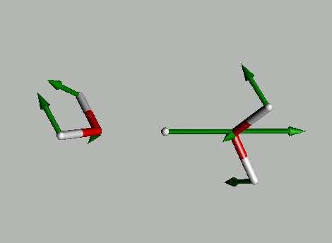
135 6.1 IR Spectra of Protonated Water Clusters Figure 6.4: Selected normal modes of the Zundel cation (H 5 O + 2 ) (referring to the corresponding stick-spectrum in Fig. 6.3(c)). 121

136 6 Test and Reference Calculations in the Gas Phase Figure 6.5: Selected normal modes of the H 7 O + 3 protonated water cluster (referring to the corresponding stick-spectrum in Fig. 6.3(d)). Figure 6.6: Selected normal modes of the Eigen cation (H 9 O 4 + ) (referring to the corresponding stick-spectrum in Fig. 6.3(e)). 122

137 6.1 IR Spectra of Protonated Water Clusters Intensity [ arbit. units ] M2 + H 5 O 2 + H 5 O 2 4H2 O M4/5/6 M3 M Wavenumber [ cm -1 ] Figure 6.7: IR spectrum of the solvated Zundel complex (H 5 O H 2 O), in comparison to that of a bare Zundel (computed under the same conditions as those in Fig. 6.3.) Figure 6.8: Selected normal modes of the solvated Zundel complex (referring to the corresponding stick-spectrum in Fig. 6.7 (blue vertical lines)). 123

138 6 Test and Reference Calculations in the Gas Phase 6.2 QM/MM Calculations The purpose of this section is to probe the quality of the QM/MM set-up by means of simple test calculations on smaller molecular systems in the gas phase. In particular, we have chosen to consider the water dimer as a prototype for an uncharged, only hydrogen-bonded system, as well as the solvated hydronium (the Eigen) as a test example for a simply charged (protonated) species [9]. For the former system, the QM part has been assigned to the hydrogen-bond donor H 2 O within the dimer (see Fig. 6.9); while for the later system the central H 3 O + within the Eigen has been taken over this role. For the QM parts, the general CPMD input parameter and keyword set-up, as listed on page 115, has been applied throughout for all the calculations, with the exception that the trajectories of the water dimer (both, QM/MM and all QM) were calculated at 100 K, since at 300 K the gas-phase water dimer dissociates into two independent water molecules. The remaining MM water molecules, on the other hand, were parametrized in terms of the SPC water model [124]. As it will turn out in the following, most of the discrepancy that are found when treating the system in either a QM/MM or in a full QM manner, can be explained from an overestimated dipole dipole interaction in-between the MM and the QM part in our QM/MM calculations. This overestimation is due to the fact that the SPC water model, used in the MM representation, is parametrized for bulk water simulations, and thus has to have a somewhat larger (static) polarization than a quantum-mechanical water molecule in the gas phase. This higher dipole moment then, of course, also tends to overpolarize the neighboring QM part, resulting, for example, in blue-shifted O H stretching modes in the IR spectrum, maxima at higher arguments in the dipole distribution function, or all-in-all in shorter atomic distances across the QM/MM border (all as compared to a pure quantum-mechanical treatment) The Water Dimer Distance Distribution [ Fig ] Extracting the corresponding distribution function from the two 10 ps trajectories, reveals that the distance between the oxygen of the donor water and that belonging to the acceptor one in average is about 0.3 Å shorter for the QM/MM calculation than for the all-qm calculation ( 2.7 vs. 3.0 Å). For a comparison, the O O distance of the water dimer, measured by molecular beam experiments, amounts to 2.98 Å [151]. 124

139 6.2 QM/MM Calculations Dipole Distribution [ Fig ] Regarding the distribution of the dipole moment of the donor H 2 O, instead, the difference between the QM/MM and the all-qm case is already less distinct: 2.02 vs Debye. The slight overpolarized QM water in the latter case can certainly be attributed to a too high dipole moment of the neighboring SPC water, as already explained above. For the sake of a reference, the dipole distribution of a single H 2 O in the gas phase was added as well (blue curve), which, with a mean value of 1.82 Debye, clearly is lying below that for the H 2 O donor within the dimer (due the absence of any mutual polarization effects). IR Spectrum [ Fig ] Also of interest is the IR spectrum of the H 2 O donor in the QM/MM case just computed (via Eq. 5.15) from the overall dipole trajectory of the QM part, and in the all-qm case by means of Wannier center decomposition techniques (according to methods discussed in Subsec ). While the bending and stretching modes do not change noteworthy in their locations, there is a striking splitting of the O H stretching peak observable for the QM/MM spectrum. This division, being also slightly present in the all-qm case, is due to the lower oscillatory frequency (i.e. weaker bonding strength) of that O H group which directs to the acceptor H 2 O, as compared the second hydroxyl group which only has a small component in the direction of O-O connection axis. This spitting tendency of the O H stretching mode in case of a QM/MM treatment of the water dimer, again is nicely explained by an overpolarization of that hydroxyl group which directs to the SPC water. Figure 6.9: Ball-and-stick model of a QM/MM water dimer. The l.h.s. (QM) H 2 O represents the hydrogen-bond donor, and the r.h.s. (MM) H 2 O the corresponding acceptor. The green balls indicate the centers of maximally localized Wannier orbitals for the QM part. 125

140 6 Test and Reference Calculations in the Gas Phase 6 5 all QM QMMM P / A R O-O / A Figure 6.10: Distance distribution in-between the two O-atoms from the all-qm (red) and the QM/MM (green) water dimer (both at a temperature of 100 K). Probability / D H 2 O donor, all-qm (100 K) H 2 O donor, QM/MM (100 K) H 2 O isolated (300 K) Dipolemoment / D Figure 6.11: Dipole probability distributions of a QM-H 2 O molecule in different environments: as a donor H 2 O within an all-qm (red) or QM/MM (green) water dimer in the gas phase at 100 K; and, for the sake of a reference, as an isolated molecule (blue) in the gas phase at 300 K. 126

141 6.2 QM/MM Calculations Intensity / arbit. units Intensity / arbit. units H 2 O donor; all-qm rot. corrected H 2 O donor; QM/MM rot. corrected Wavenumber / cm -1 Figure 6.12: IR spectrum of a donor H 2 O within an all-qm (red) and a QM/MM (green) water dimer. The rotational correction, according to Sec , is applied to the single donor H 2 O within the water dimer and not with respect to the dimer as a whole (for which this would not be necessary). 127

142 6 Test and Reference Calculations in the Gas Phase The Solvated Hydronium (Eigen Cation) Distance and Angle Distribution [ Fig ] The topology of groups like O (A) H O (B) that is, of hydrogen bonds often are visualized by a two-dimensional density plot of the mutual O O distance, R O (A) O (B), in combination with the so-called δ-coordinate, as defined by δ := R O (A) H R O H. For a molecular system where the proton resides (B) midway between O (A) and O (B) the Zundel topology is a good example for a such, the δ-coordinate should be symmetrically distributed around zero. For the Eigen cation instead, this symmetry is broken and the maximum of the δ-coordinate is expected to be 0 (i.e., more precisely, < 0 when our definition of δ is applied). The top panel of Fig displays the averaged and normalized 2-dimensional (R O O, δ) probability distribution for an all-qm and a QM/MM treated Eigen cation, respectively. 3 The general rule, that the asymmetry of of the O H O group (large δ ) tends to increase for growing O O distances, also is confirmed for the Eigen cation (for both the treatments); but the QM/MM Eigen cation shows analogous to the case of the water dimer a stronger hydrogen bonding between the hydronium QM part and the SPC waters (as deduced from a shorter mean O O distance and a smaller δ value, in comparison to the results for the all-qm Eigen). Dipole Distribution [ Fig ] The dipole distribution function of the H 3 O + subunit in the different environments, displays nearly the same kind of behavior as this was the case for the H 2 O donor within the water dimer (Fig. 6.11). When coordinated by 3 SPC waters, the induced dipole moment onto the central hydronium is the strongest; slightly stronger (i.e. overpolarized) as compared to the all-qm treatment of the Eigen. The dipole moment of a an bare hydronium in average is about 0.5 Debye lower than in the previous two cases, where polarization effects played a role. 3 The Eigen cation has three O H i O i units (i = 1, 2, 3; for the notation see Fig.6.13), which either can be considered in terms of separate (R O O i, δ i ) distributions, or, after a 3-fold averaging of the O O distances and δ coordinates, respectively, by only a single such two-dimensional distribution. By the averaging, some degree of (anti)correlation in the motion of the three subunits will certainly get lost. 128

143 6.2 QM/MM Calculations IR Spectrum [ Fig ] The IR spectrum of the hydronium in all the cases i.e., as part of an all-qm treated Eigen cation, solvated by 3 SPC waters, or in bare form always is dominated by the O H stretching band. As expected, the blue-shifts of these bands, scales with the strength of polarization that is induced from the solvation shell (as compared to the bare case). Concerning the librational modes of the H 3 O + below 600 cm 1, these are clearly observable in the bare case, still present but a little blue-shifted in the QM-solvated case, an finally almost completely suppressed in the MM-solvated case; this observation also clearly confirms that the intermolecular forces are the strongest for the QM/MM treatment. A detailed comparison of the 3 spectra in the region between 600 and 2000 cm 1, where for the gas-phase H 3 O + (see Fig. 6.3(b)) the umbrella mode at about 800 cm 1 and the bending mode(s) at about 1650 cm 1 are located, seems to be rather difficult here without further analysis. Figure 6.13: Ball-and-stick structure of a QM/MM Eigen cation. The central hydronium (H 3 O + ) unit represents the QM part, whose maximally localized Wannier centers are depicted by green balls. 129

144 6 Test and Reference Calculations in the Gas Phase all QM QM/MM < δ i > i=1,2,3 / A < R Oi -O* > i=1,2,3 / A P / Grad all QM QM/MM < α Oi -H i -O* > i=1,2,3 / Grad 130 Figure 6.14: Probability distribution of some distance- and angle parameter characterizing the geometry of an Eigen cation: all-qm Eigen (red) versus QM/MM Eigen (blue). Top: 2-dimensional distribution of the central O-atom (O ) to ligand O-atom (O i ) distance (averaged over i = 1,2,3) and the likewise averaged so-called δ-coordinate (δ i := R O H i R Oi H i ). The maxima of the distributions are indicated by the (blue and red) dashed straight lines. Bottom: 1-dimensional distribution of the averaged angle, α i, enclosed by the 3 atoms O H i O i, representing the hydrogen bonds (i = 1, 2, 3).

145 6.2 QM/MM Calculations Probability / D H 3 O + in Eigen; all QM H 3 O + in; Eigen QM/MM H 3 O + isolated Dipolemoment / D Figure 6.15: Dipole probability distribution of an hydronium (H 3 O + ) in different environments: H 3 O + as part of a all-qm (red) / QM/MM (blue) Eigen cation, and H 3 O + isolated in the gas phase (green). Intensity / arbit. units H 3 O + in Eigen; all QM H 3 O + in Eigen; QM/MM H 3 O + isolated Wavenumber / cm -1 Figure 6.16: IR spectra of a H 3 O + within the same three environments as in Fig (The green spectrum is the same as that in Fig. 6.3(b).) 131

146 6 Test and Reference Calculations in the Gas Phase 6.3 The Zundel Spectrum Investigated by Dipole Decomposition Motivated by recent experimental measurements of the IR spectrum of the protonated water dimer in the gas phase [152], 4 we were trying to understand especially the rationale for the multi-peak substructure of the broad central Zundel band in the region between 800 and 1500 wavenumbers. Figure 6.17 shows a direct comparison of our simulated Zundel spectrum with that experimentally measured by Woeste et al. [152] in a frequency range between 600 and 1900 cm 1. experimental Absorbance / arbit. units simulated Wave Number / cm -1 Figure 6.17: Gas-phase IR spectra of the Zundel cation at room temperature; black curve: measured by multi-photon photodissociation spectroscopy [152]; green curve: simulated by Car Parrinello molecular dynamics. Our normal mode analysis of the optimized Zundel structure suggests that the broad Zundel band is to be associated with the an oscillatory motion of the central H + cation along the O O connection axis of the Zundel (see Figs. 6.3 (c) and 6.4). But this intense mode, mode M4 in Fig. 6.4, is the only normal mode over a frequency range of about 1000 wavenumbers where the Zundel band shows up. This observation could, of course, be explained by the fact that the central H + experiences a very flat (and thus anharmonic) potential when moving along the O O connection axis, giving 4 But see also the (more recent) measurements on the Zundel gas-phase IR spectrum [153] and [154, 155], with results somewhat controversial to that of [152]. 132

147 6.3 The Zundel Spectrum Investigated by Dipole Decomposition rise to a very broad absorption band. But on the other hand this reasoning would not explain the observed substructure of the Zundel continuum band, being indicative for more than one local minimum in that frequency range. In the following we shall try to resolve this open question, by means of dipoledecomposition techniques applied to the Zundel IR spectrum. These decomposition techniques either rely on the concept of Wannier centers, which allow to consider local electronic contributions from different parts of the molecule separately; or else on a projection of both, nuclear and electronic degrees of freedom perpendicular as well as parallel to the Zundel s O O connection axis. For the case of the Zundel cation, the second, projectional way of dipole decomposition in our numerical experiments always has resulted in a very efficient decoupling in terms of computed IR partial spectra (i.e. in small cross terms in Eq.(5.45)); a feature which certainly makes the physical interpretation of such a decomposition more evident. The isolated Zundel IR spectrum has been subject to several theoretical / simulational studies; either employing ab initio (i.e. in general DFT-based) molecular dynamics in order to compute the gas-phase IR spectrum on the fly [156, 157, 158, 159, 160], or alternatively, being based on a not necessarily harmonic vibrational frequency analysis by means of an afore computed potential energy surface (of often reduced dimensionality) [161, 162, 163, 164, 156, 165]. Note, that in recent theoretical investigations the H 5 O 2 + has been simulated as attached to one (or more) Ar (or Ne) atom(s) [166, 150], in order to make possible direct comparison to the results of infrared multiphoton- [152, 153], respectively, infrared pre- [154, 155] dissociation spectroscopy on the Zundel cation. Figure 6.18 starts with two different kinds of decompositions applied to the total Zundel IR spectrum (being represented by the red graph in panel (a) and panel (b), respectively). In the decomposition of panel (a), the Zundel cation is subdivided in a core part (green graph) and a ligand part (blue graph); [refer to the caption of Fig for a precise meaning of these parts in terms of nuclei and Wannier centers.] This decomposition allows one to separate the overall Zundel spectrum into one part which contains the H 2 O s stretching and bending modes, and another part which still includes the librational modes below 500 cm 1, as well as the central broad Zundel continuum. In the spectral range of the O H stretching modes both parts from the decomposition in Fig (a) are distinctly anticorrelated (negative amplitude of the violet graph), allowing for the interpretation that H O stretching motions are somewhat damped by the presence of the core Zundel part. Some negative (cross-)correlation of higher amplitude also is observed in the frequency region between the H 2 O bending peak and the broad Zundel continuum band (from about 1700 to 1200 cm 1 ). 133

148 6 Test and Reference Calculations in the Gas Phase Absorbance / arbit. units (a) Zundel spectrum core part: OHO + 4WC ligand part: 4H + 4WC sum of cross terms test: = 0! Absorbance / arbit. units (b) Zundel spectrum proj. O-O axis proj. O-O axis sum of cross terms test: = 0! Wavenumber / cm -1 Figure 6.18: Two different ways of decomposing the gas-phase Zundel IR spectrum. In (a), by the use of Wannier centers (WC s), decomposition into a core Zundel part (composed out of the two oxygen atoms, the central proton, plus the 4 Wannier centers that represent the free electron pairs of the two O-atoms) and a ligand part of the Zundel (comprising the 4 outer H-atoms plus the 4 remaining Wannier centers involved in the O H bonds). In (b), projectional decomposition of both, the nuclear and the electronic degrees of freedom along and perpendicular to the O O connection axis. The violet graphs show the sum of the two cross terms from the spectral decompositions, as defined in Eq.(5.45). [The light blue zero lines just represent consistency-checks with respect to the applied spectral decomposition.] Part (b) of Fig. 6.18, instead, shows the partial spectra and cross terms from a projectional decomposition along and perpendicular to the Zundel s O O connection axis. Such a decomposition is a very proper (i.e. easy to interpret) one, since the cross terms, in from of the violet graph, are almost negligible for that case. The decomposition clearly shows that most of the spectral absorbance intensity in the overall Zundel spectrum goes back onto nuclear and electronic motion in parallel 134

149 6.3 The Zundel Spectrum Investigated by Dipole Decomposition to the O O axis; only the librational modes below 500 cm 1 (which, as we already know from the results of part (a), are generated by the core Zundel part) and the high-frequency half of the O H stretching peak are to be associated with movements in a perpendicular direction. The rationale for the double-peak structure of the O H stretching band is thus discovered by our projectional techniques so far: the parallel component of the O H motion is slightly lowered in frequency due to the hindering influence of the parallel core Zundel part; whereas this is not true for the perpendicular O H component, since there is no likewise perpendicular component from the core Zundel contributing to the IR spectrum which could induce the damping effect, such that the absorption frequency of the perpendicular component coincides with that of the O H stretching mode(s) of a free water molecule in the gas phase. In Figure 6.19, the projection into parts parallel and perpendicular to the O O connection axis is applied, but this time, to the Zundel-core (OHO+4WC) only. As to be expected from the analysis of the two foregoing decompositions in Fig. 6.18, the perpendicular core Zundel part gives rise to the librational modes in the far IR, while the parallel core Zundel part nicely incorporates just the broad continuum band with its characteristic substructure. The minor differences that are seen between the partial spectra of panel (a) and those of panel (b) in Fig. 6.19, are due to the differences in the reference point (i.e. the origin of the coordinate system) with respect to which the dipole moments were calculated in both cases. If the center of mass (COM) of the total Zundel is applied as a reference point when describing the dynamics of the core Zundel only, some slight contributions from the O H stretching modes are (artificially) re-introduced into the partial spectra (see panel (a) of Fig. 6.19). These artificial contributions are absent when, instead, the COM of the core Zundel part is employed as a reference point (as this is the case in panel (b)). Thus wee have chosen to use the latter reference point for all the following dipole decompositions of the core Zundel part. 135

150 6 Test and Reference Calculations in the Gas Phase Absorbance / arbit. units (a) OHO+4WC total OHO+4WC O-O axis OHO+4WC O-O axis sum of cross terms test: = 0! Absorbance / arbit. units (b) OHO+4WC total OHO+4WC O-O axis OHO+4WC O-O axis sum of cross terms test: = 0! Wavenumber / cm -1 Figure 6.19: Spectral decomposition of the core Zundel part in parallel and perpendicular to the O O connection axis. In (a), calculated with respect to the center of mass (COM) of the total Zundel as a reference point; and in (b), with respect to the COM of only the core Zundel part. In order to further resolve (and thereby also to better understand ) the central Zundel band, we have applied two more decompositions to the O O-parallel part of the core Zundel (OHO+4WC ). The first is shown in panel (a) of Fig. 6.20, where the OHO + 4WC part has been subdivided into nuclei a (OHO ) and an electronic (4WC ) contribution. But this decomposition has not achieved a further separation of the Zundel continuum band, with respect to the observed substructure. Both, the electronic and the nuclear degrees of freedom nearly exhibit the same pattern of peaks and valleys in the their partial spectra, adding up with a positive cross-correlation to the Zundel continuum. 136

151 6.3 The Zundel Spectrum Investigated by Dipole Decomposition Absorbance / arbit. units (a) OHO+4WC O-O axis OHO O-O axis 4WC O-O axis sum of cross terms test: = 0! Absorbance / arbit. units (b) OHO O-O axis 2O O-O axis H O-O axis sum of cross terms test: = 0! Wavenumber / cm -1 Figure 6.20: Panel (a) shows a further decomposition of the parallel part of the core Zundel into nuclei (OHO ) and electronic (4WC ) degrees of freedom. Panel (b) shows a decomposition of only the nuclear parallel part of the core Zundel (OHO ) into the two oxygens and the central proton. Due to the negative outcome of the previous dipole decomposition, we have tried, as further alternative, the subdivision of the nuclei core part only; i.e. a one into the two oxygens and the central hydrogen. But his decomposition (see Fig panel (b)) has not been successful either, in the above respect; showing only that the two ligand O-atoms are highly anticorrelated in their spectral intensity to the contribution of central proton; whose motion has, when taken alone, the strongest impact onto the IR spectrum. 137

152 6 Test and Reference Calculations in the Gas Phase As a quintessence from our dipole-decomposition investigations, we can state that the central Zundel continuum band (extending over a frequency range of approximately 700 to 1500 cm 1 ) could be traced back to the motion of the core Zundel moiety (OHO+4WC) parallel to the O O connection axis. It however turned out, that it is not possible to further ascribe some of the local absorption peaks, within the highly-structured continuum, to motions of peculiar constituents of the core Zundel moiety (neither nuclei nor electronic ones). From this observation, we have been lead to the conjecture that the pronounced substructure of the continuum band should be explainable in terms of a changing environment being experienced by the core Zundel part during a continuing molecular dynamics simulation. These environmental effects, in essence, should be describable by the orientation of the two ligand water molecules with respect to each other, as well as with respect to the O O axis. In order to quantify the later orientations, the angles α 1 (t) and α 2 (t) between the two normal vectors n 1 and n 2 (defined by the two H 2 O-planes, see Fig. 6.21) and the O O axis have been introduced. The orientation of the H 2 O- planes with respect to each other can then be read off from the dihedral angle, ξ ξ(n 1, O 1, O 2, n 2 ), defined via the directions of the two normal vectors and the position of the two O-atoms. n 1 H 2 H 1 O α 1 n 2 H O α H4 H 3 Figure 6.21: A sketch, showing the two surface normals, n 1 and n 1, defined via the two H 2 O-planes within the Zundel cation, as well as the two angle, α 1 and α 2, in-between these unit vectors and the O O connection axis. Figure 6.22 (a) shows the trajectories of the two α-angles, during a time period of half the simulation time. Striking here are the sudden jumping events of both the trajectories from values oscillating around 50 to values around 130, and vice versa. These jumps correspond to flipping events of the respective waters molecules, in the framework of which those two oxygen Wannier centers, not being involved into a covalent bond to the outer hydrogens, just mutual change their respective roles (see the illustration in Fig. 6.23). The evolution of both the angle trajectories, α 1 (t) and α 2 (t), shows that such H 2 O flipping events on both sides of the central H + are clearly correlated with respect to each other. But one cannot fully deduce from these two curves that for periods, where the angles α 1 (t) and α 2 (t) are, for instance, oscillating around the 138

153 6.3 The Zundel Spectrum Investigated by Dipole Decomposition α 1, α 2 / grad (a) t t 1 2 α 1 (t) α 2 (t) t / ps intensity / arbit. units (b) Zundel IR spec. α 1 (t) power spec. α 2 (t) power spec wavenumber / cm -1 Figure 6.22: Panel (a) shows the time evolution of the two angles α 1 (t) and α 2 (t), as sketched in Fig. 6.21, during a time span of 5 ps (half of the total MD time). Also indicated here, are the two points in MD time when the cis and trans snapshots of Fig were taken. Panel (b) shows the (y-scaled) power spectra of α 1 (t) and α 2 (t), in comparison to the complete Zundel IR spectrum. same upper (130 ) or lower (50 ) average value, the Zundel cation has to be in the cis conformation; or likewise, when the oscillation is around different average values, the trans structure has to be present (compare with Fig. 6.23). This is so, since the Zundel cation can, next to the flipping, also change its global conformation by a rotation around the O O axis. This much slower component of motion does, of course, not show up in the trajectories for α 1 (t) and α 2 (t), but should be included in the torsional (dihedral) angle, ξ(n 1, O 1, O 2, n 2 ), around the O O axis. 139

154 6 Test and Reference Calculations in the Gas Phase t = 2090 fs 1 2 t = 2130 fs cis trans Figure 6.23: Flipping event of the Zundel cation from a cis conformation into a trans one (Wannier centers in green). Both the snapshots form the same CPMD trajectory are temporally separated by about 40 f s. Figure 6.25 (a) just shows the trajectory of this dihedral angle and part (b) the corresponding distribution plot. The latter has essentially two pronounced maxima at ξ = ±90 (the inequality in the height of these two maxima is due to insufficient statistics as gained from a 10 ps trajectory). These maxima in the occupation of the torsion angle, ξ, nicely corresponds to the two low-energy conformations of the Zundel cation, as having been found previously from electronic-structure calculations [167, 168, 169] (see Fig. 6.24). Coming back now to our initial question of this Subsection, our suggestion for elucidating the origin of the Zundel s continuum band substructure, now, would be to perform some geometry-constrained molecular dynamics simulations, in which the Zundel globally is confined to one of the low-energy structures C 2 or C s (see Fig. 6.24), or to yet a third low-energy conformation exhibiting a (trivial) C 1 symmetry (being also discussed in [167]); and to check whether these simulations separately might deliver one (or more) of the 3 4 sub-peaks out of the broad Zundel continuum in their respective IR spectra. C : 2 side view top view C : s side view top ξ 90 ξ 90 view Figure 6.24: The two (approximate) C 2 and C s low energy conformations of the Zundel cation (with optimized coordinates taken from Ref. [167]). Normals to the H 2 O planes are indicated by blue arrows. Note that the torsion angle, ξ, between the two intramolecular normal vectors amounts to 90 for both structures, respectively. 140

155 6.3 The Zundel Spectrum Investigated by Dipole Decomposition Dehidral angle / grad Relative frequentness (a) t / ps (b) Dehidral angle / grad Figure 6.25: Time evolution (a) and corresponding distribution plot (b) of the dihedral angle, ξ ξ(n 1, O 1, O 2, n 2 ), defined via the two water normals (of Fig. 6.21) and the two O-atoms within the Zundel cation. 141

156

157 7 IR Spectra of Protonated Waters Clusters in BR 7.1 Electrostatics of the Glu194 /Glu204 Pocket At this point wee shall try to visualize the electrostatic environment around the so-called Glu194/Glu204 pocket, as the host of our quantum-mechanically modeled protonated water clusters. As can be seen from Fig. 2.5 (or Fig. 2.6), the Glu194 /Glu204 pocket constitutes the second (closest to the extra-cellular medium) cavity below the retinal+lysine chromophore which, in the BR ground-state, is filled with 3 channel-internal water molecules; a fourth water molecule (water 407 in Fig. 2.5) is separating that lower pocket from an upper hydrophilic pocket directly below the Schiff base. For the purpose of electrostatic investigations, the CPMD/GROMOS QM/MM interface code, used by us (see Sec. 3.3), offers the possibility of writing out (1) the electrostatic potential arising from all the MM partial charges, confined to the QM box only, and (2) the (normalized) electronic charge density from all the QM atoms, likewise computed only inside of the QM box. [These options can be invoked by specifying the keyword WRITE POTENTIAL, respectively, WRITE DENSITY in the &QMMM section of the interface s input file in the framework of a wavefunction (respectively geometry) optimization; for more details refer to the accompanying user manual]. In Figure 7.1 (a), both these quantities are depicted: the electrostatic potential in form of red and blue isosurfaces, being indicative for the presence of negative, respectively, positive (partial) charges in the vicinity of the Glu194 /Glu204 pocket; and the electronic density by means of an isosurface around the H 9 O 4 + quantum part. Note that in Fig. 7.1 (a), the isovalue determining the negative isosurfaces is much higher in absolute value than that for the positive isosurfaces ( 0.27 versus +0.05). Consequently, the visualization makes apparent that the Glu194 /Glu204 pocket is embedded in a primarily negative environment, and being thus designed, in this respect, to host protonated networks of water molecules. The dominating negative charge is essentially produced by four deprotonated carboxyl acid residues; two of these are located below the pocket, belonging to the 143

158 7 IR Spectra of Protonated Waters Clusters in BR residues Glu194 and Glu204, and the two remaining ones above it, as a part of Asp85 and Asp212. Contributions to the positive charge environment mainly arise from the single (positively) charged guanidinium head group ( C 2(NH 2 ) + ) of the arginine residues Arg82 and Arg134, respectively; or else from other polar covalent bonds close to the cavity (primarily H N bonds). Figure 7.1 (b) constitutes an alternative way in visualizing the electrostatic partial charges around the QM part, as compared to Fig. 7.1 (a), in that the electromagnetic potential here is represented by a color-projection onto an (enlarged) electrostatic density isosurface around the quantum part. Thereby, one can nicely visualize how well the Eigen cation can be embedded in this particular hydrophilic pocket. Figure 7.1: (caption referring to the two pictures on the next side) Top: electrostatic environment of the hydrophilic Glu149 /Glu204 cavity. The blue bubbles correspond to a charge isovalues of +0.05, thus indicating the location of positive partial charges; while the red bubbles have been generated by a negative isovalue of The partial charges of the central H 9 O 4 + quantum part are not visualized; the soft-gray isosurface around that protonated water cluster, instead, corresponds to an electronic density of (normalized). All the MM atoms from the first distance shell to the QM part (see Sec. 3.3) are included, sketched in a stick-like drawing mode. Bottom: same system (with same orientation) as in the top part but here, the electrostatic potential around the Glu194/Glu204 pocket is visualized by color-encoding its values on an enlarged electronic-density isosurface around the QM part (red negative partial charge nearby, blue positive partial charge nearby). 144

159 7.1 Electrostatics of the Glu194 /Glu204 Pocket Asp85 Retinal Asp212 Thr205 Arg82 Glu9 Glu204 Glu194 Arg134 Asn

160 7 IR Spectra of Protonated Waters Clusters in BR 7.2 The embedded Eigen Cation As already described in Chap. 4, during the process of classical equilibration of the overall simulated BR system, a fourth channel-internal water molecule (water 407 in Fig or Fig. 4.11), which originally was located more upward close to the phenol ring of Tyr57, entered into the Glu194/Glu204 cavity. Then, upon switching to a quantum description of the 4 waters plus one excess proton in that pocket, these constituents immediately rearranged into a stable Eigen configuration, with, more or less (see later), stable hydrogen bonding to some of the side chains of the surrounding amino acids. In detail, hydrogen bonds to the (molecular-mechanically described) residues Tyr57, Thr205, Glu204, Glu194, Tyr79 and Arg82 have been established, as can be seen from Fig During the 10 ps of QM/MM molecular dynamics necessary for recording the spectrum as shown in Fig. 7.3, no application of any kind of constrains or restrains were required, in order to preserve the protonated water cluster in a proper Eigen topology within that environment. H (b) H (a) O (2) O * O (3) H (a) Figure 7.2: Eigen-type protonated water cluster as embedded in the hydrophilic Glu194/Glu204 pocket of BR. Broken lines indicate hydrogen bonds within the Eigen cation and towards the side chains of some residues enclosing the pocket (labeled in black). The electronic structure of the protonated water network is visualized in terms of the so called electronic localization function (ELF) being apparent as darkblue transparent bubbles. The additional labeling of some of the O- and H-atoms refers to Figs. 7.4 and

161 7.2 The embedded Eigen Cation As it was to be expected, the resulting IR absorption spectrum of the Eigen cation in the Glu194/Glu204 pocket does not differ much from the gas-phase one (both are shown in Fig. 7.3); with the exceptions that firstly, the librational modes, being present in the gas phase below 500 cm 1, are largely suppressed in BR; and secondly, the dominating Eigen-peak, which in the gas phase is centered around 2700 cm 1, seems to be broaden as well as altogether slightly redshifted. The fact that the librational (hindered rotational) modes are largely absent when the Eigen cation is embedded in that BR pocket comes, of course, as no surprise. Similarly, the second feature of a broadening and red-shifting of the spectrum, certainly traces back to a weakening of the intramolecular forces between the H 3 O + core Eigen part and the 3 ligand H 2 O s, which in turn is due to the hydrogen bonding of these water molecules to the protein environment in BR gas phase Intensity / arbit. units Wave Number / cm -1 Figure 7.3: IR spectra of the Eigen-type protonated water cluster (H 3 O + 3H 2 O) in the gas phase and embedded in BR (see Fig. 7.2). Both spectra are calculated from a trajectory of 10 ps Car Parrinello MD at 300 K. The final point to be mentioned here, is that there is present some dynamics in the hydrogen bonding between the Eigen and the protein, already on the short, 10 ps time scale of our QM/MM run. By considering the time evolution of angles in Fig. 7.4 (a)+(b), it is obvious that the H 2 O molecule H-bonded between Tyr57 and Thr205 (see Fig. 7.2) swaps its H-bonding partners at about 9 ps of QM/MM 147

162 7 IR Spectra of Protonated Waters Clusters in BR MD time by rotating itself by and angle of 180 o around the O (2) O connection axis. This sudden 180 o rotation obviously was induced by a positional fluctuation of the side chain of Thr205, as it can be deduced from the perturbation (reduction) in the O (2) H (b) O (Thr205) angle (blue graph in Fig. 7.4 (b)) half a ps before the afore-mentioned swapping event. In a similar manner, Fig. 7.5 reveals that, at the same instant in MD time (at around 9 ps), the O (3) H (a) hydroxyl group of another H 2 O from the Eigen cation has changed its H-bonding partners in-between the two O-atoms of the carboxyl group of Glu (a) α O-H O / deg α O-H O / deg (b) O (2) -H O (2) -H O (2) -H O (2) -H (Tyr57) (a) O (Tyr57) (b) O (Thr205) (a) O (Thr205) (b) O t / ps Figure 7.4: Time evolution of angles spanned by the two hydroxyl groups of one of the water molecules from the Eigen cation (see the labeling in Fig.7.2) and one of the O-atoms from the carboxyl group of the Tyr57, respectively, Thr205 residue. From the evolution of these 4 graphs it is obvious that this H 2 O has rotated around the O (2) -O axis by an angle of 180 in the last quarter of the MD run, and thereby has exchanged the hydrogen bonds among the two carbonyl groups belonging to different residues. 148

163 7.2 The embedded Eigen Cation α O-H O / deg O (3) -H (a) O (Glu194) a O (3) -H (a) O (Glu194) b t / ps Figure 7.5: Time evolution of the two angles spanned by the O (3) -H (a) hydroxyl group from the Eigen cation (see the labeling in Fig.7.2) and the two O-atoms from the negatively charged carboxyl group of the Glu194 residue; revealing a jump in the hydrogen bonding (α 180 ) within that carboxyl group after around 9 ps of MD time. 149

164 7 IR Spectra of Protonated Waters Clusters in BR 7.3 The embedded Zundel Cation Motivated by the fact that, next to the Eigen cation, the Zundel topology is the second important limiting structure in H + transport via the Grotthuss mechanism (see the discussion at the beginning of Subsec ), it was challenging to verify whether also a H 2 O H + OH 2 component could be embedded in the Glu194/Glu204 pocket in a stable manner. Since the total volume of the cavity under consideration is rather large for a single Zundel cation, we have tried to incorporate a four-fold hydrated (solvated) Zundel (4H 2 O H 5 O + 2 ) into that pocket. [A bare Zundel would inevitably have been dragged to one side of the cavity by H-bonding forces, and thereby causing a disturbance in the symmetry of its O H + O core unit.] The outcome of this effort can be considered in Fig Figure 7.6: Four-fold solvated Zundel complex (H 5 O + 2 4H 2O) embedded in the same Glu194/Glu204 pocket of BR as the Eigen cation in Fig But instead of the presence of an additional (buffering) hydration shell, the core Zundel cation within that cavity turned out to be not fully stable (symmetric) nonetheless; making it necessary to apply additional constrained forces. In particular, during all of the QM/MM simulation time, the 4 oxygens from the hydration shell were distance-constrained to the 4 peripheral hydrogens of the Zundel core by 150

165 7.3 The embedded Zundel Cation a value of 1.68 Å, respectively. Beyond that, distance constraints, directly applied to the O H + O moiety for keeping it symmetric, were only used during the short period of QM/MM equilibration (and were then switched-off when data-recording started). Figure 7.7 shows the final spectrum of the hydrated Zundel within BR from a 10 ps QM/MM simulation, in comparison to that from an analogous calculation in the gas phase. As it already was the case for the Eigen cation, the libration modes below 500 cm 1 are largely suppressed when the solvated Zundel is embedded in a hydrogen bonding protein environment. On the opposite, high-frequency end of the IR spectrum, the O H stretching modes of the water molecule ligands are redshifted by an amount of 500 cm 1 with respect to the gas phase; and the contribution of these modes to the intensity of the overall spectrum is greatly enhanced as well. The central part of the absorption spectrum, on the other hand, is dominated by what usually is called the Zundel-band ; while the range over which this broad continuum absorption does extend nearly stays unaltered (roughly from 500 to 2000 cm 1 ), the distribution of local peaks and valleys within that band has changed considerably, when comparing BR-embedded and gas-phase results. Intensity / arbit. units 0.22 in BR 0.2 gas phase Wave Number / cm -1 Figure 7.7: IR spectra of the solvated Zundel complex (H 5 O + 2 4H 2O) in gas phase and embedded in BR (as seen in Fig. 7.6). Both spectra were calculated from a trajectory of 10 ps Car Parrinello MD at 300 K. The 4 distances, pairwise build between the oxygens of the H 2 O ligands and the outer hydrogens of the Zundel core, were constrained to 1.68 Å (for both the simulations, in BR and in gas phase). 151

166 7 IR Spectra of Protonated Waters Clusters in BR 7.4 Comparison with Experiments It was already mentioned that our computed IR spectra for the Eigen- and the Zundel complexes inside of BR turned out to be rather complementary with respect to each other; the broad Zundel band extends from about 500 to 2000 cm 1 and the broad resonance for the Eigen from 2000 to 3000 cm 1 (see Fig. 7.8). Provided that both these topologies of protonated water clusters simultaneously occur in BR at some stage of the photocycle (without to many disturbances from other IR absorbing sources), this dichotomy then offers the possibility to judge how large the contribution from each of the two species to the overall measured spectrum is, simply by comparing the measured spectrum to a hypothetical spectrum, that is constructed according to the following scaled superposition of intensities c [ Eigen ] + (1 c) [ Zundel ] ; c [0, 1]. (7.1) The outcome of such a superposition of Eigen- and solvated-zundel contributions to the overall IR spectrum can be considered in in Fig. 7.9, for different values of the parameter c. In experimental terms, the hypothetical overlapping of Eigen and Zundel spectra according to (7.1) could just as well be realized by means of a mixture of Eigen and Zundel-dominated BR intermediate structures in the same measuring sample. This possibility cannot be completely ruled out, especially in consideration of the fact that the duration of the UV laser pulse for collectively photo-exciting all BR molecules in a test sample falls into the same order of magnitude as that for the time resolution of the step-scan FTIR absorptional measurement (namely in the order of a few nanoseconds in both the cases, see e.g. [72]). As it already has been outlined in Chap. 2, more recent time-dependent FTIR studies on BR, in fact, provide clear evidences on the presence of broad continuum bands in intermediate-minus-groundstate difference spectra. In the L BR and K BR transient difference spectra missing absorbance (during L and K) in the range of about 2500 to 3000 cm 1 could be detected; and analogously in the range of cm 1 for the ground-state difference spectra taken with respect to the intermediates from M to O (see Fig. 2.9, and Refs. [72] and [76]). 1 Since there are two distinct continuum bands found in these measurements, separated in time and frequency domain, it is obviously more appropriate at this point to compare the two measured (difference) continuum spectra to the computed ones for the Eigen and the Zundel, individually instead of to a superposition of both according to (7.1). 1 The region below 1800 cm 1 cannot really be considered here for proofing the existence of continuum bands, because it is congested with lots of vibrational bands that result from changes within the protein itself. 152

167 7.4 Comparison with Experiments Eigen solv. Zundel Intensity / arbit. units Wavenumber / cm -1 Figure 7.8: Direct comparison between the Eigen-type (from Fig. 7.3) and the solvated Zundel-type (from Fig. 7.7) IR spectrum in BR. Figure 7.9: Superimposed Eigen-type (c = 1) and Zundel-type (c = 0) IR spectra in BR as a function of c, according to Eq. (7.1). 153