Transmission Lines. Plane wave propagating in air Y unguided wave propagation. Transmission lines / waveguides Y. guided wave propagation

Transcription

1 Transmission Lines Transmission lines and waveguides may be defined as devices used to guide energy from one point to another (from a source to a load). Transmission lines can consist of a set of conductors, dielectrics or combination thereof. As we have shown using Maxwell s equations, we can transmit energy in the form of an unguided wave (plane wave) though space. In a similar manner, Maxwell s equations show that we can transmit energy in the form of a guided wave on a transmission line. Plane wave propagating in air Y unguided wave propagation Transmission lines / waveguides Y guided wave propagation Transmission line examples

2

3 Transmission Line Definitions Almost all transmission lines have a cross-sectional geometry which is constant in the direction of wave propagation along the line. This type of transmission line is called a uniform transmission line. Uniform transmission line - conductors and dielectrics maintain the same cross-sectional geometry along the transmission line in the direction of wave propagation. Given a particular conductor geometry for a transmission line, only certain patterns of electric and magnetic fields (modes) can exist for propagating waves. These modes must be solutions to the governing differential equation (wave equation) while satisfying the appropriate boundary conditions for the fields. Transmission line mode - a distinct pattern of electric and magnetic field induced on a transmission line under source excitation. The propagating modes along the transmission line or waveguide may be classified according to which field components are present or not present in the wave. The field components in the direction of wave propagation are defined as longitudinal components while those perpendicular to the direction of propagation are defined as transverse components. Transmission Line Mode Classifications Assuming the transmission line is oriented with its axis along the z- axis (direction of wave propagation), the modes may be classified as 1. Transverse electromagnetic (TEM) modes - the electric and magnetic fields are transverse to the direction of wave propagation with no longitudinal components [E z = H z = 0]. TEM modes cannot exist on single conductor guiding

4 structures. TEM modes are sometimes called transmission line modes since they are the dominant modes on transmission lines. Plane waves can also be classified as TEM modes. 2. Quasi-TEM modes - modes which approximate true TEM modes for sufficiently low frequencies. 3. Waveguide modes - either E z, H z or both are non-zero. Waveguide modes propagate only above certain cutoff frequencies. Waveguide modes are generally undesirable on transmission lines such that we normally operate transmission lines at frequencies below the cutoff frequency of the lowest waveguide mode. In contrast to waveguide modes, TEM modes have a cutoff frequency of zero.

5 Transmission Line Equations Consider the electric and magnetic fields associated with the TEM mode on an arbitrary two-conductor transmission line (assume perfect conductors). According to the definition of the TEM mode, there are no longitudinal fields associated with the guided wave traveling down the transmission line in the z direction (E z = H z = 0). From the integral form of Maxwell s equations, integrating the line integral of the electric and magnetic fields around any transverse contour C 1 gives 0 0 where ds = dsa z. The surface integrals of E and H are zero-valued since there is no E z or H z inside or outside the conductors (PEC s, TEM mode).

6 The line integrals of E and H for the TEM mode on the transmission line reduce to These equations show that the transverse field distributions of the TEM mode on a transmission line are identical to the corresponding static distributions of fields. That is, the electric field of a TEM at any frequency has the same distribution as the electrostatic field of the capacitor formed by the two conductors charged to a DC voltage V and the TEM magnetic field at any frequency has the same distribution as the magnetostatic field of the two conductors carrying a DC current I. If we change the contour C 1 in the electric field line integral to a new path C 2 from the! conductor to the + conductor, then we find These equations show that we may define a unique voltage and current at any point on a transmission line operating in the TEM mode. If a unique voltage and current can be defined at any point on the transmission line, then we may use circuit equations to describe its operation (as opposed to writing field equations). Transmission lines are typically electrically long (several wavelengths) such that we cannot accurately describe the voltages and currents along the transmission line using a simple lumped-element equivalent circuit. We must use a distributed-element equivalent circuit which describes each short segment of the transmission line by a lumpedelement equivalent circuit.

7 Consider a simple uniform two-wire transmission line with its conductors parallel to the z-axis as shown below. Uniform transmission line - conductors and insulating medium maintain the same cross-sectional geometry along the entire transmission line. The equivalent circuit of a short segment )z of the two-wire transmission line may be represented by simple lumped-element equivalent circuit.

8 R = series resistance per unit length (S/m) of the transmission line conductors. L = series inductance per unit length (H/m) of the transmission line conductors (internal plus external inductance). G = shunt conductance per unit length (S/m) of the media between the transmission line conductors (insulator leakage current). C = shunt capacitance per unit length (F/m) of the transmission line conductors. We may relate the values of voltage and current at z and z+)z by writing KVL and KCL equations for the equivalent circuit. KVL KCL Grouping the voltage and current terms and dividing by )z gives Taking the limit as )z 6 0, the terms on the right hand side of the equations above become partial derivatives with respect to z which gives Time-domain transmission line equations (coupled PDE s)

9 For time-harmonic signals, the instantaneous voltage and current may be defined in terms of phasors such that The derivatives of the voltage and current with respect to time yield jt times the respective phasor which gives Frequency-domain (phasor) transmission line equations (coupled DE s) Note the similarity in the functional form of the time-domain and the frequency-domain transmission line equations to the respective source-free Maxwell s equations (curl equations). Even though these equations were derived without any consideration of the electromagnetic fields associated with the transmission line, remember that circuit theory is based on Maxwell s equations. Just as we manipulated the two Maxwell curl equations to derive the wave equations describing E and H associated with an unguided wave (plane wave), we can do the same for a guided (transmission line TEM) wave. Beginning with the phasor transmission line equations, we take derivatives of both sides with respect to z. We then insert the first derivatives of the voltage and current found in the original phasor transmission line equations.

10 The phasor voltage and current wave equations may be written as Voltage and current wave equations where ( is the complex propagation constant of the wave on the transmission line given by Just as with unguided waves, the real part of the propagation constant (") is the attenuation constant while the imaginary part ($) is the phase constant. The general equations for " and $ in terms of the per-unit-length transmission line parameters are The general solutions to the voltage and current wave equations are ~~~~~ ~~~~~ +z-directed waves _ a!z-directed waves

11 The coefficients in the solutions for the transmission line voltage and current are complex constants (phasors) which can be defined as The instantaneous voltage and current as a function of position along the transmission line are Given the transmission line propagation constant, the wavelength and velocity of propagation are found using the same equations as for unbounded waves. The region through which a plane wave (unguided wave) travels is characterized by the intrinsic impedance (0) of the medium defined by the ratio of the electric field to the magnetic field. The guiding structure over which the transmission line wave (guided wave) travels is characterized the characteristic impedance ( Z o ) of the transmission line defined by the ratio of voltage to current.

12 If the voltage and current wave equations defined by are inserted into the phasor transmission line equations given by the following equations are obtained. Equating the coefficients on e! ( z and e ( z gives The ratio of voltage to current for the forward and reverse traveling waves defines the characteristic impedance of the transmission line.

13 The transmission line characteristic impedance is, in general, complex and can be defined by The voltage and current wave equations can be written in terms of the voltage coefficients and the characteristic impedance (rather than the voltage and current coefficients) using the relationships The voltage and current equations become These equations have unknown coefficients for the forward and reverse voltage waves only since the characteristic impedance of the transmission line is typically known.

14 Special Case #1 Lossless Transmission Line A lossless transmission line is defined by perfect conductors and a perfect insulator between the conductors. Thus, the ideal transmission line conductors have zero resistance (F=4, R=0) while the ideal transmission line insulating medium has infinite resistance (F=0, G=0). The equivalent circuit for a segment of lossless transmission line reduces to The propagation constant on the lossless transmission line reduces to Given the purely imaginary propagation constant, the transmission line equations for the lossless line are

15 The characteristic impedance of the lossless transmission line is purely real and given by The velocity of propagation and wavelength on the lossless line are Transmission lines are designed with conductors of high conductivity and insulators of low conductivity in order to minimize losses. The lossless transmission line model is an accurate representation of an actual transmission line under most conditions.

16 Special Case #2 Distortionless Transmission Line On a lossless transmission line, the propagation constant is purely imaginary and given by The phase velocity on the lossless line is Note that the phase velocity is a constant (independent of frequency) so that all frequencies propagate along the lossless transmission line at the same velocity. Many applications involving transmission lines require that a band of frequencies be transmitted (modulation, digital signals, etc.) as opposed to a single frequency. From Fourier theory, we know that any time-domain signal may be represented as a weighted sum of sinusoids. A single rectangular pulse contains energy over a band of frequencies. For the pulse to be transmitted down the transmission line without distortion, all of the frequency components must propagate at the same velocity. This is the case on a lossless transmission line since the velocity of propagation is a constant. The velocity of propagation on the typical non-ideal transmission line is a function of frequency so that signals are distorted as different components of the signal arrive at the load at different times. This effect is called dispersion. Dispersion is also encountered when an unguided wave propagates in a non-ideal medium. A plane wave pulse propagating in a dispersive medium will suffer distortion. A dispersive medium is characterized by a phase velocity which is a function of frequency. For a low-loss transmission line, on which the velocity of propagation is near constant, dispersion may or may not be a problem, depending on the length of the line. The small variations in the velocity of propagation on a low-loss line may produce significant distortion if the line is very long. There is a special case of lossy line with the linear phase constant that produces a distortionless line.

17 A transmission line can be made distortionless (linear phase constant) by designing the line such that the per-unit-length parameters satisfy Inserting the per-unit-length parameter relationship into the general equation for the propagation constant on a lossy line gives Although the shape of the signal is not distorted, the signal will suffer attenuation as the wave propagates along the line since the distortionless line is a lossy transmission line. Note that the attenuation constant for a distortionless transmission line is independent of frequency. If this were not true, the signal would suffer distortion due to different frequencies being attenuated by different amounts. In the previous derivation, we have assumed that the per-unit-length parameters of the transmission line are independent of frequency. This is also an approximation that depends on the spectral content of the propagating signal. For very wideband signals, the attenuation and phase constants will, in general, both be functions of frequency. For most practical transmission lines, we find that RC > GL. In order to satisfy the distortionless line requirement, series loading coils are typically placed periodically along the line to increase L.

18 Transmission Line Circuit (Generator/Transmission line/load) The most commonly encountered transmission line configuration is the simple connection of a source (or generator) to a load (Z L ) through the transmission line. The generator is characterized by a voltage V g and impedance Z g while the transmission line is characterized by a propagation constant ( and characteristic impedance Z o. The general transmission line equations for the voltage and current as a function of position along the line are The voltage and current at the load (z = l ) is We may solve the two equations above for the voltage coefficients in terms of the current and voltage at the load.

19 Just as a plane wave is partially reflected at a media interface when the intrinsic impedances on either side of the interface are dissimilar (0 1 ú0 2 ), the guided wave on a transmission line is partially reflected at the load when the load impedance is different from the characteristic impedance of the transmission line (Z L úz o ). The transmission line reflection coefficient as a function of position along the line [ '(z)] is defined as the ratio of the reflected wave voltage to the transmitted wave voltage. Inserting the expressions for the voltage coefficients in terms of the load voltage and current gives The reflection coefficient at the load (z=l) is and the reflection coefficient as a function of position can be written as

20 Note that the ideal case is to have ' L = 0 (no reflections from the load means that all of the energy associated with the forward traveling wave is delivered to the load). The reflection coefficient at the load is zero when Z L = Z o. If Z L = Z o, the transmission line is said to be matched to the load and no reflected waves are present. If Z L ú Z o, a mismatch exists and reflected waves are present on the transmission line. Just as plane waves reflected from a dielectric interface produce standing waves in the region containing the incident and reflected waves, guided waves on a transmission line reflected from the load produce standing waves on the transmission line (the sum of forward and reverse traveling waves). The transmission line equations can be expressed in terms of the reflection coefficients as The last term on the right hand side of the above equations is the reflection coefficient '(z). The transmission line equations become Thus, the transmission line equations can be written in terms of voltage coefficients (V so +,V so! ) or in terms of one voltage coefficient and the reflection coefficient (V so +, '). The input impedance at any point on the transmission line is given by the ratio of voltage to current at that point. Inserting the expressions for the phasor voltage and current [V s (z) and I s (z)] from the original form of

21 the transmission line equations gives The voltage coefficients have been determined in terms of the load voltage and current as Inserting these equations for the voltage coefficients into the impedance equation gives We may use the following hyperbolic function identities to simplify this equation:

22 Dividing the numerator and denominator by cosh [((l!z)] gives Input impedance at any point along a general transmission line For a lossless line, (=j$ and Z o is purely real. The hyperbolic tangent function reduces to which yields Input impedance at any point along a lossless transmission line Special Case #1 Open-circuited lossless line (*Z L *64, ' L = 1) Special Case #2 Short-circuited lossless line (*Z L *60, ' L =!1)

23

24 The impedance characteristics of a short-circuited or open-circuited transmission line are related to the positions of the voltage and current nulls along the transmission line. On a lossless transmission line, the magnitude of the voltage and current are given by The equations for the voltage and current magnitude follow the crank diagram form that was encountered for the plane wave reflection example and the minimum and maximum values for voltage and current are For a lossless line, the magnitude of the reflection coefficient is constant along the entire line and thus equal to the magnitude of ' at the load. The standing wave ratio (s) on the lossless line is defined as the ratio of maximum to minimum voltage magnitudes (or maximum to minimum current magnitudes). The standing wave ratio on a lossless transmission line ranges between 1 and 4.

25 We may apply the previous equations to the special cases of opencircuited and short-circuited lossless transmission lines to determine the positions of the voltage and current nulls. Open-Circuited Transmission Line ( ' L =1) Current null (Z in = 4) at the load and every 8/2 from that point. Voltage null (Z in =0) at 8/4 from the load and every 8/2 from that point. Short-Circuited Transmission Line ( ' L =!1) Voltage null (Z in = 0) at the load and every 8/2 from that point. Current null (Z in = 4) at 8/4 from the load and every 8/2 from that point.

26 From the equations for the maximum and minimum transmission line voltage and current, we also find It will be shown that the voltage maximum occurs at the same location as the current minimum on a lossless transmission line and vice versa. Using the definition of the standing wave ratio, the maximum and minimum impedance values along the lossless transmission line may be written as Thus, the impedance along the lossless transmission line must lie within the range of Z o /s to sz o.

27 Example A source [V sg =100p0 o V, Z g = R g = 50 S, f = 100 MHz] is connected to a lossless transmission line [L = 0.25:H/m, C=100pF/m, l=10m]. For loads of Z L = R L = 0, 25, 50, 100 and 4 S, determine (a.) the reflection coefficient at the load (b.) the standing wave ratio (c.) the input impedance at the transmission line input terminals (d.) voltage and current plots along the transmission line.

28 R L (S) (a.) Z in (S) (b.) ' L (c.) s 0 0! !

29 R L (S) *V s (z)* max (V) *V s (z)* min (V) *V s (l)* (V)

30 R L (S) *I s (z)* max (A) *I s (z)* min (A) *I s (l)* (A)

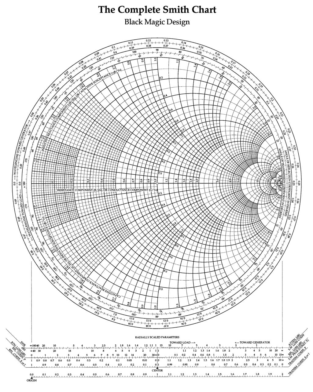
31 Smith Chart The Smith chart is a useful graphical tool used to calculate the reflection coefficient and impedance at various points on a (lossless) transmission line system. The Smith chart is actually a polar plot of the complex reflection coefficient '(z) [ratio of the reflected wave voltage to the forward wave voltage] overlaid with the corresponding impedance Z(z) [ratio of overall voltage to overall current]. The phasor voltage at any point on the lossless transmission line is The reflection coefficient at any point on the transmission line is defined as where ' L is the reflection coefficient at the load (z = l) given by where z L defines is the normalized load impedance. The magnitude of the complex-valued reflection coefficient ranges from 0 to 1 for any value of load impedance. Thus, the reflection coefficient (and corresponding impedance) can always be mapped on the unit circle in the complex plane. (1)

32 The corresponding standing wave ratio s is The magnitude of ' L is constant on any circle in the complex plane so that the standing wave ratio (VSWR) is also constant on the same circle. Smith chart center Y *' L * = 0 Constant VSWR (no reflection - matched, s = 1) circle Outer circle Y *' L * = 1 (total reflection, s = 4) Once the position of ' L is located on the Smith chart, the location of the reflection coefficient as a function of position [ '(z)] is determined using the reflection coefficient formula. This equation shows that to locate '(z), we start at ' L and rotate through an angle of 2 z =2$(z!l) on the constant VSWR circle. With the load located at z=l, moving from the load toward the generator (z < l) defines a negative angle 2 z (counterclockwise rotation on the constant VSWR circle). Note that if 2 z =!2B, we rotate back to the same point. The distance traveled along the transmission line is then Thus, one complete rotation around the Smith chart (360 o ) is equal to one half wavelength.

33 On the Smith chart... CW rotation Y toward the generator CCW rotation Y toward the load 8/2=360 o 8=720 o *'* and s are constant on a lossless transmission line. Moving from point to point on a lossless transmission line is equivalent to rotation along the constant VSWR circle. All impedances on the Smith chart are normalized to the characteristic impedance of the transmission line (when using a normalized Smith chart). The points along the constant VSWR circle represent the complex reflection coefficient at points along the transmission line. The reflection coefficient at any given point on the transmission line corresponds directly to the impedance at that point. To determine this relationship between ' L and Z L, we first solve (1) for z L. (2) where r L and x L are the normalized load resistance and reactance, respectively. Solving (2) for the resistance and reactance gives equations for the resistance and reactance circles.

34 In a similar fashion, the reflection coefficient as a function of position '(z) along the transmission line can be related to the impedance as a function of position Z(z). The general impedance at any point along the length of the transmission line is defined by the ratio of the phasor voltage to the phasor current. The normalized value of the impedance z n (z) is (3)

35 Note that Equation (2) is simply Equation (3) evaluated at z =l. (2) Thus, as we move from point to point along the transmission line plotting the complex reflection coefficient (rotating around the constant VSWR circle), we are also plotting the corresponding impedance. Once a normalized impedance is located on the Smith chart for a particular point on the transmission line, the normalized admittance at that point is found by rotating 180 o from the impedance point on the constant (3) reflection coefficient circle.

36 The locations of maxima and minima for voltages and currents along the transmission line can be located using the Smith chart given that these values correspond to specific impedance characteristics. Voltage maximum, Current minimum Y Voltage minimum, Current maximum Y Impedance maximum Impedance minimum

37

38 Example (Smith chart) A 75 S lossless transmission line of length is terminated by a load impedance of 120S. The line is energized by a source of 100V (rms) with an internal impedance of 50 S. Determine (a.) the transmission line input impedance and (b.) the magnitude of the load voltage. Using the Smith chart software, (1.) Define normalization factor for the Smith chart (Z o =75S). (2.) Define load impedance (Z L =120S). (3.) Insert series t-line (Z o =75S). (4.) Move (2.5 revolutions) on the constant VSWR circle to find Z in. (a.) DP#1 ( j0.0)s DP#2 ( j0.0)s Z in = ( j0)s

39 (b.) Using a pencil and paper Smith chart, (1.) Find the normalized load impedance. (2.) Move (2.5 revolutions) toward generator (CW) to find normalized input impedance. (3.) De-normalize the input impedance.

40 Example (Smith chart) A 60 S lossless line has a maximum impedance Z in = (180 + j0) S at a distance of 8/24 from the load. If the line is 0.38, determine (a.) s (b.) Z L and (c.) the transmission line input impedance. (a.) (b.) [Z in ] max occurs at the rightmost point on the s=3 circle. From this point, move 8/24 toward the load (CCW) to find Z L. (c.) Insert series transmission line section and from Z L, move toward the generator (CW) to find Z in.

41 DP#1 ( j78.1) S DP#2 ( j2.8) S

42 Quarter Wave Transformer When mismatches between the transmission line and load cannot be avoided, there are matching techniques that we may use to eliminate reflections on the feeder transmission line. One such technique is the quarter wave transformer. If Z o ú Z L, *'*> 0 (mismatch) Insert a 8/4 length section of different transmission line (characteristic impedance = Z o N ) between the original transmission line and the load. The input impedance seen looking into the quarter wave transformer is Solving for the required characteristic impedance of the quarter wave transformer yields

43 Example (Quarter wave transformer) Given a 300 S transmission line and a 75 S load, determine the characteristic impedance of the quarter wave transformer necessary to match the transmission line. Verify the input impedance using the Smith chart. DP#1 ( j0.0) S DP#2 ( j0.0) S

44 Stub Tuner A quarter-wave transformer is effective at matching a resistive load R L to a transmission line of characteristic impedance Z o when R L úz o. However, a complex load impedance cannot be matched by a quarter wave transformer. The stub tuner is a transmission line matching technique that can used to match a complex load. If a point can be located on the transmission line where the real part of the input admittance is equal to the characteristic admittance (Y o =Z o!1 ) of the line (Y in =Y o ±jb ), the susceptance B can be eliminated by adding the proper reactive component in parallel at this point. Theoretically, we could add inductors or capacitors (lumped elements) in parallel with the transmission line. However, these lumped elements usually are too lossy at the frequencies of interest. Rather than using lumped elements, we can use a short-circuited or open-circuited segment of transmission line to achieve any required reactance. Because we are using parallel components, the use of admittances (as opposed to impedances) simplifies the mathematics. l! length of the shunt stub d!distance from the load to the stub connection Y s! input admittance of the stub Y tl! input admittance of the terminated transmission line segment of length d Y in! input admittance of the stub in parallel

45 with the transmission line segment

46 Y tl = Y o + jb [Admittance of the terminated t-line section] Y s =!jb [Admittance of the stub (short or open circuit)] Y in = Y tl + Y s = Y o [Overall input admittance] [Transmission line characteristic admittance] In terms of normalized admittances (divide by Y o ), we have y tl = 1 + jb y s =!jb y in = 1 Note that the normalized conductance of the transmission line segment admittance (y tl = g + jb) is unity (g = 1). Single Stub Tuner Design Using the Smith Chart 1. Locate the normalized load impedance z L (rotate 180 o to find y L ). Draw the constant VSWR circle [Note that all points on the Smith chart now represent admittances]. 2. From y L, rotate toward the generator (CW) on the constant VSWR circle until it intersects the g = 1. The rotation distance is the distance d while the admittance at this intersection point is y tl = 1 + jb. 3. Beginning at the stub end (short circuit admittance is the rightmost point on the Smith chart, open circuit admittance is the leftmost point on the Smith chart), rotate toward the generator (CW) until the point at y s =!jb is reached. This rotation distance is the stub length l.

47 Short circuited stub tuners are most commonly used because a shorted segment of transmission line radiates less than an open-circuited section. The stub tuner matching technique also works for tuners in series with the transmission line. However, series tuners are more difficult to connect since the transmission line conductors must be physically separated in order to make the series connection. Example Design a short-circuited shunt stub tuner to match a load of Z L =(60! j40) S to a 50S transmission line. Short circuit admittance - rightmost point on Smith chart (0 o ) Shunt stub reactance

48