Mixed Effects Models

Transcription

1 Mixed Effects Models What is the effect of X on Y What is the effect of an independent variable on the dependent variable Independent variables are fixed factors. We want to measure their effect Random factors are variables who effect we don't want to measure, but we know it may be there. We want to eliminate it. Participants are random factors. Test items are random factors. Example of Participant affecting the outcome Research Question: What influences people to use or not use that in a sentence? Examples: I knew (that) he wouldn't show up. There are a lot of things (that) we don't know. Dependent Variable: that or no-that Independent Variables (fixed factors: Tense: past or present Sex: M, F Age 3-way: old, middle-aged, young Occupation: student, white collar, blue collar Random factor: participant Outcome without random effect of participant Tense (4.49e-32) Occ (5.97e-07) Age.3way (0.0044) Sex (0.132) Outcome with participant as random factor Tense (2.18e-31) Occ ( ) Age.3way (0.216) Sex (0.849)

2 Why does age become insignificant? Some participants were deleting that much more or less than others in their age group, which made it look like age was a factor, in reality, it was caused by a few individuals that were outliers. Repeated Measures Correlation, Chi square, independent t-test, ANOVA assume independence of (lack of correlation between) the measurements. This assumption would be violated if: 1 A single person is measured more than once Correlation of language proficiency and number of year in country. Same person's data added more than once influences outcome too much Measurements of one person's VOT to many different words taken 2 A single person belongs to more than one test group Three groups: highly fluent, intermediate, low One person is put into two different groups Linguistic data often uses repeated measurements 1 What is the effect of X on VOT? There are 10 participants, and measurements of their VOTs to many different words is taken (Participant is a random factor. We aren't interested in differences between participants) 2 What is the effect of pronunciation training on foreign accent Three groups: no pronunciation training, training X, training Y. 20 native speakers rate all members of each group on degree of accent (Rater is a random factor. We don't care about differences between raters) We aren't interested in differences in the random factor, but we must acknowledge they exist and account for them statistically, or the results are not valid!

3 Example: end up VERBing Research question: what is the effect of time on the use of end up VERBing? Dependent variable: # of end up VERBing per mission Independent variable: time Random factor: corpus (which is the subject here. It is measured several times) Time 0 is 1930s and Time 50 is 2000s (quadratic to make data linear) Regression line is best fit, predicted values Good fit if dots are close, bad if they are far away Difference between data points and regression line are residuals (What the model doesn't explain)

4 Let's pretend that there are no repeated measures only decade as a factor MODEL 1 (no compensation for repeated measures) Open end up VERBing. Analyze > Mixed Models > Linear > Continue. Put end up verbing in the dependent variable box and Decade square in the covariate box. Click on fixed and then on DecadeSq. Move it to the Model box by clicking on Add > Continue > OK Total number of parameter is 3 (from Model Dimension box) Type III Tests of Fixed Effects a Source Numerator df Denominator df F Intercept DecadeSq

5 Information Criteria a -2 Restricted Log Likelihood Akaike's Information Criterion (AIC) Hurvich and Tsai's Criterion (AICC) Bozdogan's Criterion (CAIC) Schwarz's Bayesian Criterion (BIC) Restricted log Likelihood Same as deviance in Rbrul Used to compare models Smaller is better Can use to perform log likelihood test BIC Used to compare models Smaller is better Cannot use to perform log likelihood test Formula: Calculate the -2LL of model X minus the -2LL of model Y. Look up the resulting difference in a Chi square chart by the difference in degrees of freedom between each model. -2LL degrees of freedom Model Model difference At df=1 the -2LL must be or greater to be significant at p <.05.

6

7 Notice that there is lots of correlation (lack of independence) between the corpora. Time is always higher than the rest, GoogleUK is always lower. Let's factor in subject (corpus) as a random effect by allowing each to have its own regression line. Now the residuals are measured from the data point to the individual corpus regression line. They are smaller. The individual regression lines differ in two aspects: Intercept: their average distance from the overall mean. Where they intersect with the Y axis at zero (too hard to see here). Slope: how the slant of the individual line varies from the overall regression line. Time has a steeper slope and GoogleUK has a less steep slope. There may be interaction between the intercept and the slope. Here lower intercepts are correlated with flatter slopes and higher intercepts are correlated with steeper slopes.

8 MODEL 2 (adding a random intercept) Results Analyze > Mixed Models > Linear. Move Corpus to Subjects box > Contine. Put end up verbing in the dependent variable box, Corpus in Factors box, and Decade square in the covariate box. Click on fixed and then on DecadeSq. Move it to the Model box by clicking on Add > Continue. Click on Random, then Corpus and Add to move it to the Combinations Box. Check Include Intercept. Change Covariance Type to Scaled Identity > Continue > OK. The model has a random intercept for each corpus. The regression line for each corpus is parallel to the overall regression line. Decade is still significant Information Criteria a -2 Restricted Log Likelihood Akaike's Information Criterion (AIC) Hurvich and Tsai's Criterion (AICC) Bozdogan's Criterion (CAIC) Schwarz's Bayesian Criterion (BIC) Chi square chart -2LL degrees of freedom Model Model difference At df=1 the -2LL must be or greater to be significant at p <.05. Model 2 is more complex, but has a better fit. Adding random intercepts improves fit.

9 In chart, the slope differs by corpus. Random slope may fit better

10 MODEL 3 (random slope) Analyze > Mixed Models > Linear. Move Corpus to Subjects box > Continue. Put end up verbing in the dependent variable box, Corpus in Factors box, and Decade square in the covariate box. Click on fixed and then on DecadeSq. Move it to the Model box by clicking on Add > Continue. Click on Random, then DecadeSq and Add to move it to the Model Box. Check Include Intercept. Click on Corpus and move to Combinations box with the arrow. Change Covariance Type to Scaled Identity > Continue > OK. Degrees of freedom (Parameters) = 4 Chi square chart -2LL degrees of freedom Model Model difference 62 0 At df=1(or 0) the -2LL must be or greater to be significant at p <.05. Model 3 is better fit. Decade is no longer significant! p =.052. It is the differences in corpora that cause the effect. Information Criteria a -2 Restricted Log Likelihood Akaike's Information Criterion (AIC) Hurvich and Tsai's Criterion (AICC) Bozdogan's Criterion (CAIC) Schwarz's Bayesian Criterion (BIC)

11 Practice Winter and Bergen (2012) contend that language comprehension does not uniquely involve language mechanisms but perceptual systems as well. The hypothesize that when processing a sentence that describes an object at a distance, that produces a mental image of the object that can affect the perception of a picture of that object. Their participants read sentences that described objects that were either near (e.g. While you're milking the cow it starts mooing) or far away (e.g. Across the field, the cow starts mooing). Afterwards, they were shown a picture and asked to respond yes if it matched the preceding sentence, or no if it did not. Of course, not all of the trials involved matches between sentences and picture. However, when there was a match there were actually two kinds of matching pictures: one showed the object close up and the other far away. The difference was in the size of the object in the picture. Large objects are perceived to be closer than small objects. When participants heard a sentence about a cow, they should answer yes to a picture of a cow regardless of whether the cow is depicted as being close or far away. However, the authors hypothesized that the participants would respond more quickly when the distance in the sentence matched the distance in the picture, and more slowly when there was a mismatch. This experiment involves repeated measures because each participant belongs to each of the four groups that were contrasted: far sentence, small object; far sentence, large object, close sentence, small object; close sentence, large object. In addition, each subject gave multiple responses in each of the four groups. Dependent variable: reaction time in seconds (RTinSeconds) Independent variable: Condition (far/big, far/small, near/big, near/small) Random factor: Subject Download these data. Model 1-Pretend there are no repeated measures. See if reaction time is influenced by condition. (Note: Condition in this case is a categorical variable. Put it in the factor box. Only numeric variables go in the covariate box) What are the results for condition? How many parameters (degrees of freedom)? What is the -2LL? What is the BIC?

12 What are the results for condition? not significant How many parameters (degrees of freedom)? 5 What is the -2LL? You can't use this model since it doesn't account for repeated measures What is the BIC? Model 2-Repeat the analysis, but this time give each subject a random intercept. See if reaction time is influenced by condition. (Note: Condition in this case is a categorical variable. Put it in the factor box. Only numeric variables go in the covariate box) What are the results for condition? How many parameters (degrees of freedom)? What is the -2LL? What is the BIC? Use a log likelihood test to see if this is a better model.

13 What are the results for condition? not significant How many parameters (degrees of freedom)? 6 What is the -2LL? What is the BIC? Use a log likelihood test to see if this is a better model. Model 3-Repeat the analysis, but this time give each subject a random slope. See if reaction time is influenced by condition. (Note: Condition in this case is a categorical variable. Put it in the factor box. Only numeric variables go in the covariate box) What are the results for condition? How many parameters (degrees of freedom)? What is the -2LL? What is the BIC? Use a log likelihood test to see if this is a better model.

14 What are the results for condition? not significant How many parameters (degrees of freedom)? 6 What is the -2LL? What is the BIC? Use a log likelihood test to see if this is a better model. No, it is worse Model 4-Repeat the analysis, but this time give each test item a random intercept. See if reaction time is influenced by condition. (Note: Condition in this case is a categorical variable. Put it in the factor box. Only numeric variables go in the covariate box) What are the results for condition? How many parameters (degrees of freedom)? What is the -2LL? What is the BIC? Use a log likelihood test to see if this is a better model compared to Model 1.

15 What are the results for condition? not significant How many parameters (degrees of freedom)? 6 What is the -2LL? What is the BIC? Use a log likelihood test to see if this is a better model compared to Model 1. Model Model Significantly smaller. Adding 1 df is justifiable.

16 Model 5-Repeat the analysis, but this time give each test item a random slope. See if reaction time is influenced by condition. (Note: Condition in this case is a categorical variable. Put it in the factor box. Only numeric variables go in the covariate box) What are the results for condition? How many parameters (degrees of freedom)? What is the -2LL? What is the BIC? Use a log likelihood test to see if this is a better model compared to Model 4.

17 What are the results for condition? not significant How many parameters (degrees of freedom)? 6 What is the -2LL? What is the BIC? Use a log likelihood test to see if this is a better model compared to Model 4. Model Model (assume 1) No significant difference, BIC got bigger, so random slope doesn't help get a better fit.

18 Using the Syntax Editor Menus are confusing. You are not sure what you are doing. The syntax editor is easier to modify. Let's start by using the menus, then see what they give us as syntax. Analyze > Mixed Models > Linear. Move Subject to Subjects box > Continue. Put RtinSeconds in the dependent variable box and Condition and Subject in the Factors box. Click on Fixed and then on Condition. Move it to the Model box by clicking on Add > Continue. Click on Random, then Condition and Add to move it to the Model Box. Check Include Intercept. Click on Subject and move to Combinations box with the arrow. Change Covariance Type to Scaled Identity > Continue > Paste (This puts it into the syntax editor). Syntax The variables in our model are in green MIXED RTinSeconds BY Subject CONDITION /CRITERIA=CIN(95) MXITER(100) MXSTEP(10) SCORING(1) SINGULAR( ) HCONVERGE(0, ABSOLUTE) LCONVERGE(0, ABSOLUTE) PCONVERGE( , ABSOLUTE) /FIXED=CONDITION SSTYPE(3) /METHOD=REML /RANDOM=INTERCEPT CONDITION SUBJECT(Subject) COVTYPE(ID). MIXED: run a mixed effects model RtinSeconds: dependent variable BY: specifies the categorical independent variables Subject CONDITION: the categorical independent variables (both fixed and random) WITH: specifies the numeric independent variables (there are none so there is no WITH here) /CRITERIA=CIN(95) MXITER(100) MXSTEP(10) SCORING(1) SINGULAR( ) HCONVERGE(0, ABSOLUTE) LCONVERGE(0, ABSOLUTE) PCONVERGE( , ABSOLUTE): Directions to the computer on how to run the analysis. /FIXED: What the fixed effects are. CONDITION: the independent variable

19 SSTYPE(3): More directions to the computer. /METHOD=REML: More directions to the computer /RANDOM: What the random effects are INTERCEPT: calculate the intercept CONDITION SUBJECT(Subject): Calculate a random slope for each subject across each of the test conditions in CONDITION. COVTYPE(ID): Type of variance covariance matrix (Scaled identity). We'll talk about it. It is very important to put a period at the end of the syntax Random slope /RANDOM=INTERCEPT CONDITION SUBJECT(Subject) COVTYPE(ID). Random intercept /RANDOM=INTERCEPT SUBJECT(Subject) COVTYPE(ID). Running the syntax Highlight all of the syntax and press the green arrow. Look at the results in the Output window. Changing the syntax You can add and delete variables by deleting of typing them in the correct place. Practice 1 Change the syntax so that it runs a random intercept model 2 Change the syntax so that it runs a random intercept model with ITEM as the random factor instead of Subject. 3 We found that a random intercept for test item and a random intercept for subject produced a better model fit. Make a model that contains both random of these factors together. Compare the outcome to Models 2 and 4 above using a log likelihood test.

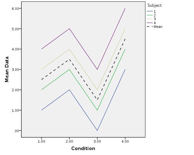
20 If each of these data points came from different people we wouldn't assume that there would be any correlation between any two points. We would measure the residuals to the overall predicted regression line.

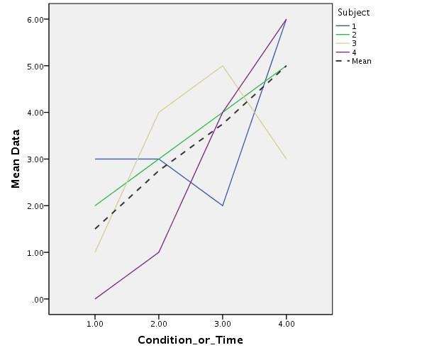
21 When one person provides more than one data point, chances are that his/her responses to one item or at one point in time are correlated. To account for this we include a random factor. When this is done the residuals are measured to the individual's predicted response (the individual's regression line).

22 The repeated statement We can sometimes fit a model even better by providing information about how the residuals are structured. A covariance structure contains two kinds of data. First, it specifies information about any correlations that exist between repeated measurements. Second, it indicates what the variance of those measurements is like across time, or across experimental condition. Two graphs above, the variance goes up over time and the covariance get larger from one decade to the next. (Covariance is unstandardized correlation. It isn't +1 to -1, but given in the units of measurement.) 1930s 1940s 1950s 1960s 1970s 1980s 1990s 2000s 1930s s s s s s s s The covariance of a covariance is the variance and appears in bold along the diagonal. If we did a correlation they would all be 1. ARH1 Heterogenous first-order autoregressive This means the variance changes over time (or conditions), and the covariance does also. It assumes that the covariance between two adjacent decades is more similar that between more distant ones.

23 CS Compound symmetry The variance is about the same across time (or condition) and the covariance is about the same. 1930s 1940s 1950s 1960s 1970s 1980s 1990s 2000s 1930s s s s s s s s 1654

24

25 ID Scaled Identity The variance is the same across time (or conditions) and there is no covariance.

26

27 Common covariance structures. Covariance Structure Variance across repeated measures Covariance across repeated measures Acronym Compound Symmetry Constant Constant CS Heterogenous Compound Symmetry Different Constant CSH Unstructured Different Different UN Autoregressive Constant Closer measurements are more correlated than distant ones. Heterogenous Autoregressive Different Covariance grow smaller with each successive measurement. Toeplitz Constant Adjacent measurements have same covariance, but covariance is smaller for nonadjacent measurements. Identity Constant None ID AR1 ARH1 Diagonal Different None DIAG TP Other covariance structures: TPH, CSR, AD1, FA1, FAH1, HF, UNR Which one do you use? The one that fits best.

28 Practice 1 Open these data. 2 Open the syntax editor and paste in the code below. File > New > Syntax. MIXED Score WITH Decade /CRITERIA=CIN(95) MXITER(100) MXSTEP(10) SCORING(1) SINGULAR( ) HCONVERGE(0, ABSOLUTE) LCONVERGE(0, ABSOLUTE) PCONVERGE( , ABSOLUTE) /FIXED=Decade SSTYPE(3) /METHOD=REML /RANDOM=INTERCEPT Decade SUBJECT(Subject) COVTYPE(ID). This is a random slope model. 3 Run this model and note the number of parameters, the -2LL, and the BIC. 4 Modify the syntax to run a random intercept model. Determine which is a better fit. 5 Add the random statement to the end and be sure to delete unnecessary periods. Run this model. /REPEATED=Decade SUBJECT(Subject) COVTYPE(DIAG). 6 Try the model with different covariance structures to see which give the best fit.