UNIVERSITY OF TORONTO. Faculty of Arts and Science APRIL 2010 EXAMINATIONS STA 303 H1S / STA 1002 HS. Duration - 3 hours. Aids Allowed: Calculator

Transcription

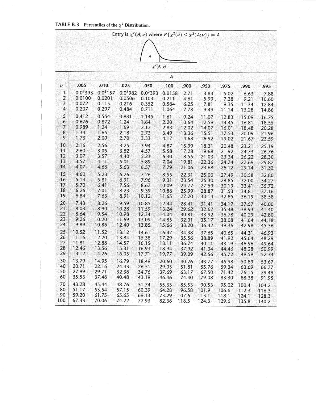
1 UNIVERSITY OF TORONTO Faculty of Arts and Science APRIL 2010 EXAMINATIONS STA 303 H1S / STA 1002 HS Duration - 3 hours Aids Allowed: Calculator LAST NAME: FIRST NAME: STUDENT NUMBER: There are 27 pages including this page. The last page is a table of formulae that may be useful. For all questions you can assume that the results on the formula page are known. A table of the chi-square distribution can be found on page 26. Total marks: 90 1abcd 1efg 1hi 2ab 2cde 2fghi 3a 3bcdef 4abcd 4efg 5 1

2 1. A study was carried out to investigate the effects of heredity and environment on intelligence. From adoption registers, researchers selected samples of adopted children whose biological parents and adoptive parents came from either the very highest or the very lowest socio-economic status (SES) categories. They attempted to obtain samples of size 10 from each combination (1. high adoptive SES and high biological SES, 2. high adoptive SES and low biological SES, 3. low adoptive SES and high biological SES, and 4. low SES for both parents). However, only 8 children belonged to combination 3. The 38 selected children were given intelligence quotient (IQ) tests. Some output from SAS for this analysis is given below and on the next 2 pages. The variables adoptive and biologic each take on the values High and Low, indicating the SES of the respective parents IQ Mean Std N adoptive biologic High High Low Low High Low Dependent Variable: IQ The GLM Procedure Class Level Information Class Levels Values adoptive 2 High Low biologic 2 High Low Number of Observations Read 38 Number of Observations Used 38 Sum of Source DF Squares Mean Square F Value Pr > F Model (A) (C) Error (B) (D) Corrected Total R-Square Coeff Var Root MSE IQ Mean Output continues on the next page 2

3 (Question 1 continued) Source DF Type I SS Mean Square F Value Pr > F adoptive biologic adoptive*biologic Source DF Type III SS Mean Square F Value Pr > F adoptive biologic adoptive*biologic Dependent Variable: IQ The GLM Procedure Class Level Information Class Levels Values adoptive 2 High Low biologic 2 High Low Number of Observations Read 38 Number of Observations Used 38 Sum of Source DF Squares Mean Square F Value Pr > F Model Error Corrected Total R-Square Coeff Var Root MSE IQ Mean Source DF Type I SS Mean Square F Value Pr > F adoptive biologic Source DF Type III SS Mean Square F Value Pr > F adoptive biologic Level of IQ adoptive N Mean Std Dev High Low Least Squares Means adoptive IQ LSMEAN High Low Output continues on the next page 3

4 (Question 1 continued) Questions begin on the next page. 4

5 (Question 1 continued) (a) (4 marks) Some numbers in the SAS output on page 2 have been replaced by letters. What are the missing values? (A) = (B) = (C) = (D) = (b) (1 mark) Two linear models have been fit in the output above. In the first linear model, how many β s (coefficients of terms in the linear model) must be estimated? (c) (2 marks) Why can the first model be considered a saturated model? Explain why, in this case, it is possible to carry out inference. (d) (2 marks) What is being tested by the test with p-value ? What do you conclude? 5

6 (Question 1 continued) (e) (2 marks) For the second linear model, some Least Squares Means are given. Explain clearly how they are calculated. (f) (2 marks) Why does one of the Least Squares Means differ from the means given in the table above the least squares means? (g) (3 marks) From the results of this study, what do you conclude about the relationship between parental socio-economic status and IQ? Quote relevant p-values to support your conclusions. 6

7 (Question 1 continued) (h) (3 marks) The first graph on page 4 is a plot of the mean IQ of the children, classified by the socio-economic status of their adoptive and biological parents. Explain how it illustrates your conclusions from part (g). (i) (4 marks) Do you trust your conclusions from part (g)? Why or why not? 7

8 2. Some of the debate about capital punishment in the U.S. has revolved around the rôle race plays in the decision to use it. The 674 subjects considered in this question were the defendants in murder cases in Florida between 1976 and SAS output for 4 models is given below and on the next 3 pages. The variables are: V - the race of the victim (either black (B) or white (W)) D - the race of the defendant (either black (B) or white (W)) C - verdict for capital punishment (yes (Y) or no (N)) MODEL 1 The GENMOD Procedure Model Information Distribution Poisson Link Function Log Dependent Variable count Number of Observations Read 8 Number of Observations Used 8 Class Level Information Class Levels Values V 2 B W D 2 B W C 2 N Y Criteria For Assessing Goodness Of Fit Criterion DF Value Value/DF Deviance Scaled Deviance Pearson Chi-Square Scaled Pearson X Log Likelihood Full Log Likelihood AIC (smaller is better) AICC (smaller is better) BIC (smaller is better) Algorithm converged. Analysis Of Maximum Likelihood Parameter Estimates Standard Wald 95% Confidence Wald Parameter DF Estimate Error Limits Chi-Square Pr > ChiSq Intercept <.0001 V B <.0001 V W D B <.0001 D W C N <.0001 C Y Scale

9 (Question 2 continued) MODEL 2 The GENMOD Procedure Model Information Distribution Poisson Link Function Log Dependent Variable count Number of Observations Read 8 Number of Observations Used 8 Class Level Information Class Levels Values V 2 B W D 2 B W C 2 N Y Criteria For Assessing Goodness Of Fit Criterion DF Value Value/DF Deviance Scaled Deviance Pearson Chi-Square Scaled Pearson X Log Likelihood Full Log Likelihood AIC (smaller is better) AICC (smaller is better) BIC (smaller is better) Algorithm converged. Analysis Of Maximum Likelihood Parameter Estimates Standard Wald 95% Wald Parameter DF Estimate Error Confidence Limits Chi-Square Pr > ChiSq Intercept <.0001 V B <.0001 V W D B <.0001 D W C N <.0001 C Y V*D B B <.0001 V*D B W V*D W B V*D W W

10 (Question 2 continued) MODEL 3 The GENMOD Procedure Model Information Distribution Poisson Link Function Log Dependent Variable count Number of Observations Read 8 Number of Observations Used 8 Class Level Information Class Levels Values V 2 B W D 2 B W C 2 N Y Criteria For Assessing Goodness Of Fit Criterion DF Value Value/DF Deviance Scaled Deviance Pearson Chi-Square Scaled Pearson X Log Likelihood Full Log Likelihood AIC (smaller is better) AICC (smaller is better) BIC (smaller is better) Algorithm converged. Analysis Of Maximum Likelihood Parameter Estimates Standard Wald 95% Wald Parameter DF Estimate Error Confidence Limits Chi-Square Pr > ChiSq Intercept <.0001 V B <.0001 V W D B <.0001 D W C N <.0001 C Y V*C B N V*C B Y V*C W N V*C W Y V*D B B <.0001 V*D B W V*D W B V*D W W Scale

11 (Question 2 continued) MODEL 4 The GENMOD Procedure Model Information Distribution Poisson Link Function Log Dependent Variable count Number of Observations Read 8 Number of Observations Used 8 Class Level Information Class Levels Values V 2 B W D 2 B W C 2 N Y Criteria For Assessing Goodness Of Fit Criterion DF Value Value/DF Deviance Scaled Deviance Pearson Chi-Square Scaled Pearson X Log Likelihood Full Log Likelihood AIC (smaller is better) AICC (smaller is better). BIC (smaller is better) Algorithm converged. Analysis Of Maximum Likelihood Parameter Estimates Standard Wald 95% Wald Parameter DF Estimate Error Confidence Limits Chi-Square Pr > ChiSq Intercept <.0001 V B <.0001 V W D B <.0001 D W C N <.0001 C Y V*D B B <.0001 V*D B W V*D W B V*D W W D*C B N D*C B Y D*C W N D*C W Y V*C B N <.0001 V*C B Y V*C W N V*C W Y

12 (Question 2 continued) (a) (4 marks) For each of the 4 models for which output is given, give a practical interpretation of the relationships among the variables (assuming that the model is appropriate). (b) (4 marks) Show how the value for the Full Log Likelihood is calculated for model 1. Give your answer in terms of the observed counts y ijk. 12

13 (Question 2 continued) (c) (1 mark) For model 1, explain why the degrees of freedom for the Criteria For Assessing Goodness Of Fit is 4. (d) (5 marks) Use a likelihood ratio test to compare the fits of models 1 and 3. State the null and alternative hypotheses, the test statistic, the distribution of the test statistic under the null hypothesis, the p-value, and your conclusion. (e) (4 marks) Carry out the Deviance Goodness-of-Fit test for model 3. State the null and alternative hypotheses, the test statistic, the distribution of the test statistic under the null hypothesis, the p-value, and your conclusion. 13

14 (Question 2 continued) (f) (2 marks) Using model 4, what is the estimated count of the number of cases with a verdict of capital punishment for which the defendant and victim were both white? (g) (3 marks) Using model 4, estimate the odds of receiving a verdict in favour of capital punishment if the defendant was black. (h) (4 marks) For model 4, what evidence is available from the SAS output that the model is adequate? What else would you like to see to ensure that the Wald tests are appropriate? (i) (2 marks) Which of the 4 models would you choose for these data? Why? 14

15 3. Below is some additional output analysing the data from question 2. ncapital is the number of cases for which the verdict was for capital punishment. MODEL A The LOGISTIC Procedure Model Information Response Variable (Events) ncapital Response Variable (Trials) m Model binary logit Optimization Technique Fisher s scoring Number of Observations Read 4 Number of Observations Used 4 Sum of Frequencies Read 674 Sum of Frequencies Used 674 Response Profile Ordered Binary Total Value Outcome Frequency 1 Event 68 2 Nonevent 606 Class Level Information Class Value Design Variables V B 1 W 0 D B 1 W 0 Model Convergence Status Quasi-complete separation of data points detected. WARNING: The maximum likelihood estimate may not exist. WARNING: The LOGISTIC procedure continues in spite of the above warning. Results shown are based on the last maximum likelihood iteration. Validity of the model fit is questionable. Model Fit Statistics Intercept Intercept and Criterion Only Covariates AIC SC Log L Testing Global Null Hypothesis: BETA=0 Test Chi-Square DF Pr > ChiSq Likelihood Ratio <.0001 Score Wald Output for MODEL A continues on the next page. 15

16 (Question 3 continued) Output for MODEL A continued Type 3 Analysis of Effects Wald Effect DF Chi-Square Pr > ChiSq V D V*D Analysis of Maximum Likelihood Estimates Standard Wald Parameter DF Estimate Error Chi-Square Pr > ChiSq Intercept <.0001 V B D B V*D B B Association of Predicted Probabilities and Observed Responses Percent Concordant 35.3 Somers D Percent Discordant 9.1 Gamma Percent Tied 55.6 Tau-a Pairs c MODEL B The LOGISTIC Procedure Model Information (SOME OUTPUT OMITTED HERE THAT IS THE SAME AS FOR MODEL A) Model Convergence Status Convergence criterion (GCONV=1E-8) satisfied. Model Fit Statistics Intercept Intercept and Criterion Only Covariates AIC SC Log L Testing Global Null Hypothesis: BETA=0 Test Chi-Square DF Pr > ChiSq Likelihood Ratio <.0001 Score <.0001 Wald Output for MODEL B continues on the next page. 16

17 (Question 3 continued) Output for MODEL B continued Type 3 Analysis of Effects Wald Effect DF Chi-Square Pr > ChiSq V <.0001 D Analysis of Maximum Likelihood Estimates Standard Wald Parameter DF Estimate Error Chi-Square Pr > ChiSq Intercept <.0001 V B <.0001 D B Odds Ratio Estimates Point 95% Wald Effect Estimate Confidence Limits V B vs W D B vs W Association of Predicted Probabilities and Observed Responses Percent Concordant 35.3 Somers D Percent Discordant 9.1 Gamma Percent Tied 55.6 Tau-a Pairs c (a) (4 marks) Give test statistics and p-values for two tests comparing models A and B. What do you conclude? (As part of your conclusion, you should be choosing one of model A or B.) 17

18 (Question 3 continued) (b) (2 marks) For the model you chose in part (a), describe the relationship among the 3 variables. (c) (2 marks) Using model B, estimate the odds of receiving a verdict in favour of capital punishment if the defendant and victim were both black. (d) (2 marks) The SAS output for model A includes the message below. Explain what the message indicates. Quasi-complete separation of data points detected. WARNING: The maximum likelihood estimate may not exist. WARNING: The LOGISTIC procedure continues in spite of the above warning. Results shown are based on the last maximum likelihood iteration. Validity of the model fit is questionable. (e) (2 marks) For model A, what are the hypotheses for the likelihood ratio test under the heading Testing Global Null Hypothesis: BETA=0 in the SAS output? What do you conclude? (f) (2 marks) Do you prefer the analysis carried out on these data in question 2 or question 3? Why? 18

19 4. A study followed the orthodontic growth of 27 children (16 males and 11 females). At ages 8, 10, 12, and 14, the distance (in millimeters) from the center of the pituitary to pterygomaxillary fissure was measured. The investigators were interested in how the growth of this distance varied as the boys and girls grew. In the analysis below, age was treated as a categorical variable. Some SAS output is given below for 3 models that were fit to the resulting data. MODEL I The Mixed Procedure Model Information Dependent Variable distance Covariance Structure Compound Symmetry Subject Effect subject(sex) Estimation Method REML Residual Variance Method Profile Fixed Effects SE Method Model-Based Degrees of Freedom Method Between-Within Class Level Information Class Levels Values sex 2 Female Male subject 27 F01 F02 F03 F04 F05 F06 F07 F08 F09 F10 F11 M01 M02 M03 M04 M05 M06 M07 M08 M09 M10 M11 M12 M13 M14 M15 M16 age Dimensions Covariance Parameters 2 Columns in X 15 Columns in Z 0 Subjects 27 Max Obs Per Subject 4 Number of Observations Number of Observations Read 108 Number of Observations Used 108 Number of Observations Not Used 0 Iteration History Iteration Evaluations -2 Res Log Like Criterion Convergence criteria met. Output for MODEL I continues on the next page. 19

20 (Question 4 continued) Output for MODEL I continued Estimated R Correlation Matrix for subject(sex) F01 Female Row Col1 Col2 Col3 Col Covariance Parameter Estimates Cov Parm Subject Estimate CS subject(sex) Residual Fit Statistics -2 Res Log Likelihood AIC (smaller is better) AICC (smaller is better) BIC (smaller is better) Null Model Likelihood Ratio Test DF Chi-Square Pr > ChiSq <.0001 Type 3 Tests of Fixed Effects Num Den Effect DF DF F Value Pr > F age <.0001 sex age*sex

21 (Question 4 continued) MODEL II (The output was edited to remove Class Level Information and Number of Observations (both same as model I) and Iteration History (convergence criteria were met).) The Mixed Procedure Model Information Dependent Variable distance Covariance Structures Variance Components, Autoregressive Subject Effect subject(sex) Estimation Method REML Residual Variance Method Profile Fixed Effects SE Method Model-Based Degrees of Freedom Method Containment Dimensions Covariance Parameters 3 Columns in X 15 Columns in Z 27 Subjects 1 Max Obs Per Subject 108 Estimated R Correlation Matrix for subject(sex) F01 Female Row Col1 Col2 Col3 Col Covariance Parameter Estimates Cov Parm Subject Estimate subject(sex) AR(1) subject(sex) Residual Fit Statistics -2 Res Log Likelihood AIC (smaller is better) AICC (smaller is better) BIC (smaller is better) Type 3 Tests of Fixed Effects Num Den Effect DF DF F Value Pr > F age <.0001 sex age*sex

22 (Question 4 continued) MODEL III (The output was edited to remove Class Level Information and Number of Observations (both same as models I and II) and Iteration History (convergence criteria were met).) The Mixed Procedure Model Information Dependent Variable distance Covariance Structure Unstructured Subject Effect subject(sex) Estimation Method REML Residual Variance Method None Fixed Effects SE Method Model-Based Degrees of Freedom Method Between-Within Dimensions Covariance Parameters 10 Columns in X 15 Columns in Z 0 Subjects 27 Max Obs Per Subject 4 Estimated R Correlation Matrix for subject(sex) F01 Female Row Col1 Col2 Col3 Col Fit Statistics -2 Res Log Likelihood AIC (smaller is better) xxxxx AICC (smaller is better) BIC (smaller is better) Null Model Likelihood Ratio Test DF Chi-Square Pr > ChiSq <.0001 Type 3 Tests of Fixed Effects Num Den Effect DF DF F Value Pr > F age <.0001 sex age*sex

23 (Question 4 continued) (a) (1 mark) The models include the interaction of sex and age. Explain in practical terms why this was included in the models. (b) (2 marks) The model was fit using the mixed models procedure in SAS. Explain why the model is mixed. (c) (4 marks) Write the model that was fit in model I, carefully defining all terms. (Do not write the fitted equation; write the model in terms of its parameters.) (d) (2 marks) For model I, why is the number of covariance parameters equal to 2? 23

24 (Question 4 continued) (e) (1 mark) What is the value of AIC for model III? (f) (2 marks) AR(1) is a commonly used covariance structure in situations such as this, where observations are taken over time. Explain why it is not an appropriate covariance structure for these data by comparing at least 2 different kinds of information given in the SAS output. (g) (2 marks) How do the conditions for valid inference for this model differ from the conditions needed for a multiple linear regression model? 24

25 5. (a) (6 marks) In order for inferences to be valid, conditions must be met. Assume standard analyses that were taught in this course are being carried out. i. Give two examples of conditions that must be met for both analysis of variance and binomial logistic regression models in order for the inferences to be valid. ii. Give two examples of conditions that must be met for the inferences to be valid for an analysis of variance model but which are not necessary for a binomial logistic regression model. iii. Give two examples of conditions that must be met for the inferences to be valid for a binomial logistic regression model but which are not necessary for an analysis of variance model. (b) (4 marks) Here are two recent quotes from lecture. What does it mean if you make predictions from a fitted model that does not adequately describe the data? Only do inference on valid models. Imagine it is sometime in the future and you have been hired to do the statistical analysis on the data collected from a scientific study. How will the ideas behind these quotes affect the work you will do? And why is this important? 25

26 26

27 Some formulae: Pooled t-test Test for two proportions / t obs = y 1 y ( ) 2 z 1 obs = (ˆπ 1 ˆπ 2 ) ˆπ p (1 ˆπ p ) s p + 1 n1 n2 n 1 n 2 b 1 = (Xi X)(Y i Y ) (Xi X) 2 = Xi Y i nxy X 2 i nx 2 Linear Regression b 0 = Y b 1 X One-way analysis of variance SSTO = N i=1 (Y i Y ) 2 SSE = G g=1 (g) (Y i Y g ) 2 SSR = G g=1 n g (Y g Y ) 2 Bernoulli and Binomial distributions If Y Bernoulli(π) If Y Binomial(m, π) E(Y ) = π, Var(Y ) = π(1 π) E(Y ) = mπ, Var(Y ) = mπ(1 π) Logistic Regression with Binomial Response formulae Deviance = 2 n i=1 {y i log(y i ) + (m i y i ) log(m i y 1 ) y i log(ŷ i ) + (m i y i ) log(m i ŷ 1 )} { ( ) ( )} D res,i = sign(y i m iˆπ i ) 2 y i log yi m iˆπ i + (m i y i ) log mi y i m i m iˆπ i P res,i = y i m iˆπ i miˆπ i (1 ˆπ i ) Multinomial distribution for 2 2 table Poisson distribution n! Pr (Y = y) = y 11!y 12!y 21!y 22! πy πy πy πy Pr(Y = y) = µy e µ y!, y = 0, 1, 2,... E(Y ) = µ, Var(Y ) = µ Two-way contingency tables (easily generalizable to three-way tables) X 2 = J Ii=1 (y ij ˆµ ij ) 2 j=1 ˆµ ij G 2 = 2 J ( ) Ii=1 yij j=1 y ij log ˆµ ij { ( ) } yij D res,ij = sign(y ij ˆµ ij ) 2 y ij log ˆµ ij y ij + ˆµ ij P res,ij = y ij ˆµ ij ˆµij AIC = 2 log(l) + 2p Model Fitting Criteria SC = 2 log(l) + p log(n) 27 Total pages 27 Total marks 90