Basic Statistics Exercises 66

Transcription

1 Basic Statistics Exercises 66

2 42. Suppose we are interested in predicting a person's height from the person's length of stride (distance between footprints). The following data is recorded for a random sample of 5 people: Length of Stride (inches) Height (inches) (a) Identify the dependent (response) variable and the independent (explanatory) variable for a regression analysis. The dependent (response) variable is Y = height, and the independent (explanatory) variable is stride length. (b) Does the data appear to be observational or experimental? Since the ages look random, it appears that the data is observational. (c) Use the formulas from Exercise 41 find the equation of the least squares line. ^ y = x (d) Use the least squares line to predict the height of a person whose length of stride is 15 inches. ^ y = (15) = 58.2 inches Basic Statistics Exercises 67

3 43. The prediction of a male's right-hand grip strength from age is to be studied. A 0.05 significance level is to be used with a simple linear regression. The following data is recorded for a random sample of males: Age (years) Grip Strength (lbs.) (a) Identify the dependent (response) variable and the independent (explanatory) variable for a regression analysis. The dependent (response) variable is Y = grip strength, and the independent (explanatory) variable is age. (b) Does the data appear to be observational or experimental? Since the ages look random, it appears that the data is observational. (c) In order to use SPSS to do the calculations needed for the statistical analysis, enter the data into an SPSS data file named age_grip containing two variables named age and grip. Then, go to the document titled Using SPSS for Windows (which can be accessed from the appropriate link on the course syllabus web page), go to the section titled Hypothesis Tests Involving Two Variables, and read the steps in the subsection titled Performing a Simple Linear Regression with Checks of Linearity, Homoscedasticity, and Normality Assumptions. Use these steps as a guide to obtaining the output needed for the remainder of this exercise. Once you have successfully generated SPSS output, add a title to the top of the output in the following format: YOUR NAME Basic Statistics Exercise 43(c) Verify that your SPSS output contains all of the following: Basic Statistics Exercises 68

4 43. - continued Basic Statistics Exercises 69

5 43. - continued Basic Statistics Exercises 70

6 43. - continued (b) Use the SPSS output to find each of the following: n = r = (11)(4.824) 2 = (c) Use the SPSS output to find the equation of the least squares line. ^ The least squares line can be written y = x. (d) Write a one-sentence interpretation of the slope in the least squares line. Grip strength appears to increase on average by about 2 pounds with each increase of one year in age. (e) Find the coefficient of determination, and write a one-sentence interpretation. From the SPSS output, we find r 2 = About 59.3% of the variation in grip strength is explained by age. (f) Find the standard error of estimate. From the SPSS output, we find s = Basic Statistics Exercises 71

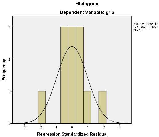
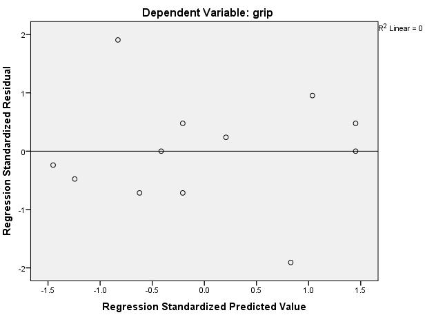
7 43. - continued (g) Use the SPSS output to make a statement concerning whether each of the following assumptions in a simple linear regression is satisfied: the linearity assumption The data points appear to be randomly distributed about the least squares line on the scatter plot, and the residuals plotted against the predicted values look random. Consequently, the linearity assumption appears to be satisfied. the uniform variance (homoscedasticity) assumption The variation in standardized residuals around the horizontal line looks reasonably uniform. the normality assumption The histogram of standardized residuals looks somewhat bell-shaped, and the points on the normal probability plot do not seem to depart too far from the diagonal line. Since the necessary assumptions appear to be satisfied, we feel it is appropriate to proceed with the regression analysis. Basic Statistics Exercises 72

8 43 - continued (h) A 0.05 significance level is chosen for a hypothesis test to see if there is any evidence that the linear relationship between age and grip strength is significant, that is, that the slope in the regression is significantly different from zero (0). Write the results of this hypothesis test two different ways: Write the results of the f test in the ANOVA table in a format suitable for a journal article to be submitted for publication. The f test in the ANOVA for the regression to predict grip strength from age is statistically significant at the 0.05 level (f 1, 10 = , f 1, 10; 0.05 = 4.96, < p < 0.01 OR p = 0.003). We conclude that the linear relationship between age and grip strength is significant, and the data suggest a positive relationship. Write the results of the t test about the slope in a format suitable for a journal article to be submitted for publication. With a t test, the sample slope (2.00 lbs.) is statistically significantly different from zero at the 0.05 level (t 10 = 3.814, t 10; = 2.228, < p < 0.01 OR p = 0.003). We can be 95% confident that the slope in the regression to predict grip strength from age is between and lbs. Considering the results of the hypothesis test, decide whether or not a 95% confidence interval for the slope in the regression would be of interest. If yes, find and interpret the confidence interval; if not, explain why. Since rejecting H 0 suggests that the hypothesized zero slope is not correct, a 95% confidence interval will provide us with some information about the slope, which estimates the average change in grip strength with an increase of one year in age. 2 (2.228)(8.390/ ), 2 + (2.228)(8.390/ ) Basic Statistics Exercises 73

9 43 - continued (i) A 0.05 significance level is chosen for a hypothesis test to see if there is any evidence that the mean grip strength for 20 year old right-handed males is different from 80 lbs. Write the results of this hypothesis test in a format suitable for a journal article to be submitted for publication. With a t test, the estimated mean grip strength (66 lbs.) is statistically significantly different from the hypothesized mean (80 lbs.) at the 0.05 level (t 10 = 5.304, t 10; = 2.228, p < 0.001). We can be 95% confident that the mean grip strength for 20 year old right-handed males is between and lbs. Considering the results of the hypothesis test, decide whether or not a 95% confidence interval for the mean grip strength for 20 year old right-handed males would be of interest. If yes, find and interpret the confidence interval; if not, explain why. Since rejecting H 0 suggests that the hypothesized mean grip strength for 20 year old right-handed males is not correct, a 95% confidence interval will provide us with some information about this mean (20) = (2.228)( /12 + (20 18) 2 /255.98), 66 + (2.228)(8.390/ 1/12 + (20 18) 2 /255.98) Basic Statistics Exercises 74

10 43 - continued (j) Find and interpret a 95% prediction interval for the grip strength of a 20 year old right-handed male (20) = (2.228)( /12 + (20 18) 2 /255.98), 66 + (2.228)(8.390/ 1 + 1/12 + (20 18) 2 /255.98) We are 95% confident that the grip strength for a randomly selected 20-year old right-handed male will be between and lbs. OR At least 95% of 20-year old right-handed males have a grip strength between and lbs. (k) For what age group of right-handed males will the confidence interval for mean grip strength and the prediction interval for a particular grip strength both have the smallest length? 18 year olds Basic Statistics Exercises 75

11 44. The prediction of score (0-100) on a test from hours of study is to be studied. A 0.05 significance level is to be used with a simple linear regression. The following data is recorded for a random sample of students: Study Time(hrs) Test Score(points) (a) Identify the dependent (response) variable and the independent (explanatory) variable for a regression analysis. The dependent (response) variable is Y = test score, and the independent (explanatory) variable is study time. (b) Does the data appear to be observational or experimental? Since the times do not look random, it appears that the data is experimental. (c) In order to use SPSS to do the calculations needed for the statistical analysis, enter the data into an SPSS data file named time_score containing two variables named time and score. Then, go to the document titled Using SPSS for Windows (which can be accessed from the appropriate link on the course syllabus web page), go to the section titled Hypothesis Tests Involving Two Variables, and read the steps in the subsection titled Performing a Simple Linear Regression with Checks of Linearity, Homoscedasticity, and Normality Assumptions. Use these steps as a guide to obtaining the output needed for the remainder of this exercise. Once you have successfully generated SPSS output, add a title to the top of the output in the following format: YOUR NAME Basic Statistics Exercise 44(c) Verify that your SPSS output contains all of the following: a scatter plot displaying the least squares line; tables titled Descriptive Statistics, Correlations, Model Summary, ANOVA, and Coefficients; a normal probability plot; a histogram on which a bell-shaped curve has been superimposed; a plot of standardized predicted values versus standardized residuals. Basic Statistics Exercises 76

12 44 - continued (b) Use the SPSS output to find each of the following: n = r = (14)(2.928) 2 = (c) Use the SPSS output to find the equation of the least squares line. ^ The least squares line can be written y = x. (d) Write a one-sentence interpretation of the slope in the least squares line. Test score appears to increase on average by about points with each increase of one hour in study time. (e) Find the coefficient of determination, and write a one-sentence interpretation. From the SPSS output, we find r 2 = About 28.1% of the variation in test score is explained by study time. (f) Find the standard error of estimate. From the SPSS output, we find s = Basic Statistics Exercises 77

13 44. - continued (g) Use the SPSS output to make a statement concerning whether each of the following assumptions in a simple linear regression is satisfied: the linearity assumption Since the data points appear to be randomly distributed about the least squares line on the scatter plot, and the residuals plotted against the predicted values look random. Consequently, the linearity assumption appears to be satisfied. the uniform variance (homoscedasticity) assumption The variation in standardized residuals around the horizontal line looks reasonably uniform. the normality assumption The histogram of standardized residuals looks somewhat bell-shaped, even though the points on the normal probability plot do not seem to depart too far from the diagonal line. Since the necessary assumptions do not appear to be drastically violated, we feel it is appropriate to proceed with the regression analysis. Basic Statistics Exercises 78

14 44 - continued In the Word document named Basic_Statistics_Result_Summaries (created previously), begin a section titled Basic Statistics Exercises 44. In this section, create a subsection for each of parts (h), (i), and (j) which follow, and in each subsection created, write the summaries for the corresponding part. Print the page(s) and insert them immediately after this page. (h) A 0.05 significance level is chosen for a hypothesis test to see if there is any evidence that the linear relationship between study time and test score is significant, that is, that the slope in the regression is significantly different from zero (0). Write the results of this hypothesis test two different ways: Write the results of the f test in the ANOVA table in a format suitable for a journal article to be submitted for publication. Write the results of the t test about the slope in a format suitable for a journal article to be submitted for publication. Also, considering the results of this hypothesis test, decide whether or not a 95% confidence interval for the slope in the regression would be of interest. If yes, find and interpret the confidence interval; if not, explain why. (i) A 0.05 significance level is chosen for a hypothesis test to see if there is any evidence that the mean test score for students who study for 5 hours is different from 85 points. Write the results of this hypothesis test in a format suitable for a journal article to be submitted for publication. Considering the results of the hypothesis test, decide whether or not a 95% confidence interval for the mean test score for students who study for 5 hours would be of interest. If yes, find and interpret the confidence interval; if not, explain why. (j) Find and interpret a 95% prediction interval for the test score of a student who studied for 5 hours. (k) For what study time will the confidence interval for mean test score and the prediction interval for a particular test score both have the smallest length? 6 hours Basic Statistics Exercises 79

15 45. In a study of the impact of temperature during the summer months on the maximum amount of power that must be generated to meet demand each day, the prediction of daily peak power load (megawatts) from daily high temperature (degrees Fahrenheit) is of interest. Data for 25 randomly selected summer days is stored in the SPSS data file powerloads (which can be accessed from the appropriate link on the course syllabus web page). A 0.05 significance level is chosen for hypothesis testing. (a) Identify the dependent (response) variable and the independent (explanatory) variable for a regression analysis. The dependent (response) variable is Y = daily peak power load, and the independent (explanatory) variable is X = daily high temperature. (b) Does the data appear to be observational or experimental? Since the daily high temperature is random, the data is observational. (c) Use SPSS to do the calculations needed for a simple linear regression by going to the document titled Using SPSS for Windows (which can be accessed from the appropriate link on the course syllabus web page), going to the section titled Hypothesis Tests Involving Two Variables, and reading the steps in the subsection titled Performing a Simple Linear Regression with Checks of Linearity, Homoscedasticity, and Normality Assumptions. Once you have successfully generated SPSS output, add a title to the top of the output in the following format: YOUR NAME Basic Statistics Exercise 45(c) Verify that your SPSS output contains all of the following: Basic Statistics Exercises 80

16 45. - continued Basic Statistics Exercises 81

17 45. - continued Basic Statistics Exercises 82

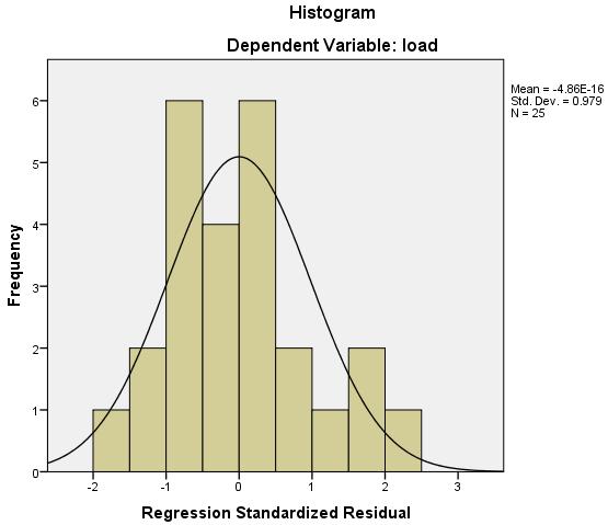
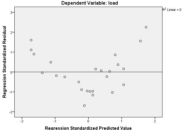
18 45. - continued (d) Use the SPSS output to make a statement concerning whether each of the following assumptions in a simple linear regression is satisfied: the linearity assumption The data points do not appear to be randomly distributed about the least squares line on the scatter plot; it seems that as temperature increases, power load increases at a faster rate. Also, the residuals plotted against the predicted values do not look random. Consequently, the linearity assumption does not appear to be satisfied. the uniform variance (homoscedasticity) assumption the normality assumption Since the linearity assumption does not appear to be satisfied, it is not possible (or even relevant) to consider the uniform variance and normality assumptions. We do not feel it is appropriate to proceed with the regression analysis. Basic Statistics Exercises 83

19 45 - continued (e) It is decided that a quadratic model to predict daily peak power load from daily high temperature will be considered to improve prediction. Write an equation which describes this model. Y = a + b 1 X + b 2 X 2 OR powerload = a + b 1 (temp) + b 2 (temp) 2 (f) Use SPSS to do the calculations needed for a quadratic regression by going to the document titled Using SPSS for Windows (which can be accessed from the appropriate link on the course syllabus web page), going to the section titled Hypothesis Tests Involving Two or More Variables, and reading the steps in the subsection titled Performing a Quadratic Regression with Checks of Model, Homoscedasticity, and Normality Assumptions. Once you have successfully generated SPSS output, add a title to the top of the output in the following format: YOUR NAME Basic Statistics Exercise 45(f) Verify that your SPSS output contains all of the following: Basic Statistics Exercises 84

20 45 - continued Basic Statistics Exercises 85

21 45 - continued (g) Use the SPSS output to make a statement concerning whether each of the following assumptions in the quadratic regression is satisfied: the assumption of the quadratic model Since the residuals plotted against the predicted values look random, the assumption of the quadratic model appears to be correct. the uniform variance (homoscedasticity) assumption The variation in standardized residuals around the horizontal line looks reasonably uniform. the normality assumption The histogram of standardized residuals looks somewhat bell-shaped, and the points on the normal probability plot do not seem to depart to far from the diagonal line. Based on these observations, we feel it is appropriate to proceed with the quadratic regression analysis. (h) A 0.05 significance level is chosen for the following hypothesis tests: First, write the results of the f test in the ANOVA table for the quadratic regression in a format suitable for a journal article to be submitted for publication. The f test in the ANOVA for the regression to predict power load from temperature and squared temperature is statistically significant at the 0.05 level (f 2, 22 = , f 2, 22; 0.05 = 3.44, p < 0.001). Basic Statistics Exercises 86

22 45(h) - continued Next, complete the steps outlined below to calculate the f statistic for the hypothesis test see if there is any evidence that the addition of squared temperature (the quadratic term) after temperature (the linear term) is statistically significant; the, write the results of this f test in a format suitable for a journal article to be submitted for publication. SSR(temp, temp 2 ) = the regression sum of squares from the ANOVA table with both temperature and squared temperature in the model = SSR(temp) = the regression sum of squares from the ANOVA table with only temperature in the model = MSE(temp, temp 2 ) = the error mean square from the ANOVA table with both temperature and squared temperature in the model = numerator df for the f statistic = number of new terms added to the model = denominator df for the f statistic = df associated with MSE(temp, temp 2 ) = SSR(temp, temp 2 ) SSR(temp) f statistic = = = MSE(temp, temp 2 ) The addition of squared temperature after temperature to predict power load is statistically significant at the 0.05 level (f 1, 22 = , f 1, 22; 0.05 = 4.30, p < 0.001). Basic Statistics Exercises 87

23 45 - continued (i) Use the SPSS output to find the equation of the least squares quadratic. The least squares line can be written ^ load = (temp) (temp) 2. (j) Find the multiple R 2, and write a one-sentence interpretation. From the SPSS output, we find R 2 = About 95.9% of the variation in power load is explained by temperature and squared temperature. (k) Find the standard error of estimate. From the SPSS output, we find s = (l) Use the least squares quadratic to predict the daily peak power load on a day when the high temperature is 75 degrees Fahrenheit, and also on a day when the high temperature is 85 degrees Fahrenheit (75) (75) 2 = megawatts (85) (85) 2 = megawatts Basic Statistics Exercises 88

24 46. In a study to predict IgG (milligrams of immunoglobulin in blood), which is an indicator of long-term immunity, from maximal oxygen uptake (milliliters per kilogram), which is a measure of aerobic fitness level, data is taken on randomly selected subjects and stored in the SPSS data file aerobic (which can be accessed from the appropriate link on the course syllabus web page). A 0.05 significance level is chosen for hypothesis testing. (a) Identify the dependent (response) variable and the independent (explanatory) variable for a regression analysis. The dependent (response) variable is Y = IgG, and the independent (explanatory) variable is X = maximal oxygen uptake. (b) Does the data appear to be observational or experimental? Since the maximal oxygen uptake is random, the data is observational. (c) Use SPSS to do the calculations needed for a simple linear regression by going to the document titled Using SPSS for Windows (which can be accessed from the appropriate link on the course syllabus web page), going to the section titled Hypothesis Tests Involving Two Variables, and reading the steps in the subsection titled Performing a Simple Linear Regression with Checks of Linearity, Homoscedasticity, and Normality Assumptions. Once you have successfully generated SPSS output, add a title to the top of the output in the following format: YOUR NAME Basic Statistics Exercise 46(c) Verify that your SPSS output contains all of the following: a scatter plot displaying the least squares line; tables titled Descriptive Statistics, Correlations, Model Summary, ANOVA, and Coefficients; a normal probability plot; a histogram on which a bell-shaped curve has been superimposed; a plot of standardized predicted values versus standardized residuals. Basic Statistics Exercises 89

25 46. - continued (d) Use the SPSS output to make a statement concerning whether each of the following assumptions in a simple linear regression is satisfied: the linearity assumption The data points do not appear to be randomly distributed about the least squares line on the scatter plot; it seems that as maximal oxygen uptake increases, IgG increases at a slower rate. Also, the residuals plotted against the predicted values do not look random. Consequently, the linearity assumption does not appear to be satisfied. the uniform variance (homoscedasticity) assumption the normality assumption Since the linearity assumption does not appear to be satisfied, it is not possible (or even relevant) to consider the uniform variance and normality assumptions. We do not feel it is appropriate to proceed with the regression analysis. Basic Statistics Exercises 90

26 46 - continued (e) It is decided that a quadratic model to predict IgG from maximum oxygen intake will be considered to improve prediction. Write an equation which describes this model. Y = a + b 1 X + b 2 X 2 OR IgG = a + b 1 (maxoxy) + b 2 (maxoxy) 2 (f) Use SPSS to do the calculations needed for a quadratic regression by going to the document titled Using SPSS for Windows (which can be accessed from the appropriate link on the course syllabus web page), going to the section titled Hypothesis Tests Involving Two or More Variables, and reading the steps in the subsection titled Performing a Quadratic Regression with Checks of Model, Homoscedasticity, and Normality Assumptions. Once you have successfully generated SPSS output, add a title to the top of the output in the following format: YOUR NAME Basic Statistics Exercise 46(f) Verify that your SPSS output contains all of the following: tables titled Descriptive Statistics, Correlations, Model Summary, ANOVA, and Coefficients; a normal probability plot; a histogram on which a bell-shaped curve has been superimposed; a plot of standardized predicted values versus standardized residuals. Basic Statistics Exercises 91

27 46 - continued (g) Use the SPSS output to make a statement concerning whether each of the following assumptions in the quadratic regression is satisfied: the assumption of the quadratic model Since the residuals plotted against the predicted values look random, the assumption of the quadratic model appears to be correct. the uniform variance (homoscedasticity) assumption The variation in standardized residuals around the horizontal line looks reasonably uniform. the normality assumption The histogram of standardized residuals looks somewhat bell-shaped, and the points on the normal probability plot do not seem to depart to far from the diagonal line. Based on these observations, we feel it is appropriate to proceed with the quadratic regression analysis. (h) A 0.05 significance level is chosen for the following hypothesis tests: First, write the results of the f test in the ANOVA table for the quadratic regression in a format suitable for a journal article to be submitted for publication. The f test in the ANOVA for the regression to predict IgG from maximal oxygen intake and squared maximal oxygen intake is statistically significant at the 0.05 level (f 2, 27 = , f 2, 27; 0.05 = 3.35, p < 0.001). Basic Statistics Exercises 92

28 46(h) - continued Next, complete the steps outlined below to calculate the f statistic for the hypothesis test see if there is any evidence that the addition of squared maximal oxygen intake (the quadratic term) after maximal oxygen intake (the linear term) is statistically significant; the, write the results of this f test in a format suitable for a journal article to be submitted for publication. SSR(maxoxy, maxoxy 2 ) = the regression sum of squares from the ANOVA table with both maximal oxygen intake and squared maximal oxygen intake in the model = SSR(maxoxy) = the regression sum of squares from the ANOVA table with only maximal oxygen intake in the model = MSE(maxoxy, maxoxy 2 ) = the error mean square from the ANOVA table with both maximal oxygen intake and squared maximal oxygen intake in the model = numerator df for the f statistic = number of new terms added to the model = denominator df for the f statistic = df associated with MSE(maxoxy, maxoxy 2 ) = f statistic = SSR(maxoxy, maxoxy 2 ) SSR(maxoxy) = = MSE(maxoxy, maxoxy 2 ) The addition of squared maximum oxygen intake after maximum oxygen intake to predict IgG is statistically significant at the 0.05 level (f 1, 27 = , f 1, 27; 0.05 = 4.21, p < 0.001). Basic Statistics Exercises 93

29 46 - continued (i) Use the SPSS output to find the equation of the least squares quadratic. The least squares line can be written ^ IgG = (maxoxy) 0.536(maxoxy) 2. (j) Find the multiple R 2, and write a one-sentence interpretation. From the SPSS output, we find R 2 = About 93.8% of the variation in IgG is explained by maximum oxygen intake and squared maximum oxygen intake. (k) Find the standard error of estimate. From the SPSS output, we find s = (l) Use the least squares quadratic to predict the the IgG for a person whose maximal oxygen uptake is 40 milliliters per kilogram (40) 0.536(40) 2 = milligrams Basic Statistics Exercises 94