Model Order Reduction of Electrical Circuits with Nonlinear Elements

Size: px

Start display at page:

Download "Model Order Reduction of Electrical Circuits with Nonlinear Elements"

Ella York
6 years ago
Views:

1 Model Order Reduction of Electrical Circuits with Nonlinear Elements Tatjana Stykel and Technische Universität Berlin July, 21

2 Model Order Reduction of Electrical Circuits with Nonlinear Elements Contents: Introduction, Motivation Tatjana Stykel and Model equations for electrical circuits with nonlinear elements Model Technische order reduction Universität Berlin Software package: PABTEC July, 21 Numerical tests Summary

3 Contents: Introduction, Motivation Model equations for electrical circuits with nonlinear elements Model order reduction Software package: PABTEC Numerical tests Summary

4 Introduction While the structural size of the electrical devices is decreasing, the complexity of the electrical circuits is increasing.

5 Introduction While the structural size of the electrical devices is decreasing, the complexity of the electrical circuits is increasing. This leads to a system of model equations consisting up to millions or even more unknowns.

6 Introduction While the structural size of the electrical devices is decreasing, the complexity of the electrical circuits is increasing. This leads to a system of model equations consisting up to millions or even more unknowns. Simulation of such large models is mostly impossible or, at least, unacceptably time and storage consuming.

7 Introduction While the structural size of the electrical devices is decreasing, the complexity of the electrical circuits is increasing. This leads to a system of model equations consisting up to millions or even more unknowns. Simulation of such large models is mostly impossible or, at least, unacceptably time and storage consuming. Model order reduction presents a way out of this dilemma.

8 Introduction While the structural size of the electrical devices is decreasing, the complexity of the electrical circuits is increasing. This leads to a system of model equations consisting up to millions or even more unknowns. Simulation of such large models is mostly impossible or, at least, unacceptably time and storage consuming. Model order reduction presents a way out of this dilemma. A general idea of model order reduction is to replace a large-scale system by a much smaller model which approximates the input-output relation of the large-scale system within a required accuracy.

9 Contents: Introduction, Motivation Model equations for electrical circuits with nonlinear elements Model order reduction Software package: PABTEC Numerical tests Summary

10 Model equations E(x) d x = Ax + f (x) + Bu, dt y = B T x,

11 Model equations E(x) d x = Ax + f (x) + Bu, dt y = B T x, states x = [ η T ı T L ıt V inputs u = [ ı T I uv T outputs y = [ ui T ı T V ] T ] T ] T

12 Model equations E(x) d x = Ax + f (x) + Bu, dt y = B T x, states x = [ η T ı T L ıt V inputs u = [ ı T I u T V ] T ] T ] T outputs y = [ ui T ı T V A C C(A T C η)at C E(x) = L(ı L ), A L A V A = A T L, A T V A R g(a T R η) f (x) =, A I B =. I

13 Model equations E(x) d x = Ax + f (x) + Bu, dt y = B T x, C, R, L, V, I as index denote conductors, resistors, inductors, voltage sources, current sources η vector of node potentials ı vector of currents u vector of volatages A incidence matrices C conductance matrix-valued function L inductance matrix-valued function g resistor relation states x = [ η T ı T L ıt V inputs u = [ ı T I u T V ] T ] T ] T outputs y = [ ui T ı T V A C C(A T C η)at C E(x) = L(ı L ), A L A V A = A T L, A T V A R g(a T R η) f (x) =, A I B =. I

14 Model equations - Assumption We will assume that (A1) the matrix A V has full column rank, (A2) the matrix [A C, A L, A R, A V ] has full row rank,

15 Model equations - Assumption We will assume that (A1) the matrix A V has full column rank, (A2) the matrix [A C, A L, A R, A V ] has full row rank, (A3) the matrices C(A T C η) and L(ı L) are positive definite for all admissible η and ı L, and (A4) the function g(a T R η) is monotonically increasing for all admissible η.

16 Model equations - Assumption We will assume that (A1) the matrix A V has full column rank, (A2) the matrix [A C, A L, A R, A V ] has full row rank, (A3) the matrices C(A T C η) and L(ı L) are positive definite for all admissible η and ı L, and (A4) the function g(a T Rη) is monotonically increasing for all admissible η. Assumptions (A1) and (A2) imply that the circuit does not contain loops of voltage sources and cutsets of current sources, respectively, while assumptions (A3) and (A4) on the capacitance and inductance matrices and the resistor relation mean that all circuit elements do not generate energy.

17 Model equations - Assumption Furthermore, we assume without loss of generality that the circuit elements are ordered such that A C = [ A C ] A C, AL = [ A L A L A R = [ ] A R, A R ], We also assume that the linear and nonlinear elements are not mutually connected, i.e., [ ] [ ] C L C(A T C η) =, L(ı L ) =, C(A η) L(ı T C L) [ ḠA T R g(a T R η) = η ], g(a T Rη)

18 Model equations Consequentely, we have the model equations in the form E(x) d x = Ax + f (x) + Bu, dt y = B T x, with A CA T C C + A C(A η)a C T C T C L E(x) = L(ı L), f (x) = A RḠAT R A L A A L V A = A T L A T L, B = A T V A I I A R g(a T Rη).,

19 Contents: Introduction, Motivation Model equations for electrical circuits with nonlinear elements Model order reduction Software package: PABTEC Numerical tests Summary

20 Model Order Reduction - Approach nonlinear circuit equations

21 Model Order Reduction - Approach nonlinear circuit equations linear subsystem Decoupling nonlinear subsystem

22 Model Order Reduction - Approach nonlinear circuit equations linear subsystem Decoupling Model order reduction (e.g. PABTEC) nonlinear subsystem reduced linear subsystem

23 Model Order Reduction - Approach nonlinear circuit equations linear subsystem Decoupling Model order reduction (e.g. PABTEC) nonlinear subsystem Recoupling reduced linear subsystem reduced nonlinear system

24 Model Order Reduction - Decoupling :-( possibly creation of LI-cutsets :-) :-( possibly creation of LI-cutsets

25 Model Order Reduction - Decoupling :-/ introduction of additional variables :-) :-( possibly creation of CV-loops

26 Model Order Reduction - Decoupling :-/ introduction of additional variables :-) :-/ introduction of additional nodes

27 Model Order Reduction - Decoupling Decoupling

28 Model Order Reduction - Decoupling Let A R { 1,, 1} nη,n R be an incidence matrix. Then the matrices A 1 R and A 2 R are uniquely defined with A 1 R {, 1} nη,n R and A 2 R { 1, } nη,n R satisfying A 1 R + A 2 R = A R. Furthermore, let ı L R n L, u C R n C, and ı z R n R be defined by the relations with the notation L(ı L) d dt ı L = A T L η, (1) u C = A T C η, (2) ı z = Γ s G 1 1 ( g(at Rη) Γ 12 A T Rη) (3) Γ s = G 1 + G 2, Γ 12 = G 1 (G 1 + G 2 ) 1 G 2.

29 Model Order Reduction - Decoupling Then the original system of model equations together with the relations η z = Γ 1 s ((G 1 (A 1 R) T G 2 (A 2 R) T )η ı z ), (4a) ı C = C(u C) d dt u C (4b) is equivalent to the linear system d A C CA T C dt η A 11 A 12 A L A V A C d dt η z L d dt ı L d dt ı = A T 12 Γ s A T L V A T V d dt ı A C T C A I A 2 R A L ı I I ı z + ı L I u V, I y 1 y 2 y 3 y 4 y 5 A T I (A 2 R) T I = A T L I I η η z ı L ıv ı C u C η η z ı L ıv ı C (5a) (5b)

30 Model Order Reduction - Decoupling Then the original system of model equations together with the relations η z = Γ 1 s ((G 1 (A 1 R) T G 2 (A 2 R) T )η ı z ), (4a) ı C = C(u C) d dt u C (4b) is equivalent to the linear system d A C CA T C dt η A 11 A 12 A L A V A C d dt η z L d dt ı L d dt ı = A T 12 Γ s A T L V A T V d dt ı A C T C A I A 2 R A L ı I I ı z + ı L I u V, I y 1 y 2 y 3 y 4 y 5 A T I (A 2 R) T I = A T L I I η η z ı L ıv ı C u C with A 11 η η z ı L ıv ı C (5a) = A R GAT R A1 RG 1 (A 1 R) T A 2 RG 2 (A 2 R) T, A 12 = A 1 RG T 1 A 2 R(G 2 ) T (5b)

31 Model Order Reduction - Decoupling Then the original system of model equations together with the relations η z = Γ 1 s ((G 1 (A 1 R) T G 2 (A 2 R) T )η ı z ), (4a) ı C = C(u C) d dt u C (4b) is equivalent to the linear system d A C CA T C dt η A 11 A 12 A L A V A C d dt η z L d dt ı L d dt ı = A T 12 Γ s A T L V A T V d dt ı A C T C A I A 2 R A L ı I I ı z + ı L I u V, I Keep in mind y 1 y 2 y 3 y 4 y 5 A T I (A 2 R) T I = A T L I I η η z ı L ıv ı C u C with A 11 η η z ı L ıv ı C y 2 = (A 2 R) T η η z y 3 = A A 2 RG T Lη 2 (A 2 R) T, Ay 12 = A Andreas 1 RG 1 T A Steinbrecher 2 R(G 5 = ı C 2 ) T (5a) = A R GAT R A1 RG 1 (A 1 R) T (5b)

32 Model Order Reduction - Model reduction of the linear subsystem Application of a model order reduction methode like PABTECL yields the reduced-order model ı I Ê d dt ˆx = Âˆx + [ ] ı z ˆB 1 ˆB 2 ˆB 3 ˆB 4 ˆB 5 ı L u V, (6a) u C ŷ = Ĉ 1 Ĉ2 Ĉ3 Ĉ4 Ĉ5 ˆx. Keep in mind (6b) y 2 = (A 2 R) T η η z y 3 = A T Lη y 5 = ı C

33 Model Order Reduction - Model reduction of the linear subsystem Application of a model order reduction methode like PABTECL yields the reduced-order model ı I Ê d dt ˆx = Âˆx + [ ] ı z ˆB 1 ˆB 2 ˆB 3 ˆB 4 ˆB 5 ı L u V, u C ŷ 1 Ĉ 1 ŷ 2 Ĉ2 ŷ 3 ŷ 4 = Ĉ3 ˆx. Ĉ4 ŷ 5 Ĉ5 Keep in mind y 2 = (A 2 R) T η η z y 3 = A T Lη y 5 = ı C

34 Model Order Reduction - Model reduction of the linear subsystem Application of a model order reduction methode like PABTECL yields the reduced-order model ı I Ê d dt ˆx = Âˆx + [ ] ı z ˆB 1 ˆB 2 ˆB 3 ˆB 4 ˆB 5 ı L u V, u C y 1 ŷ 1 Ĉ 1 y 2 y 3 y 4 ŷ 2 Ĉ2 ŷ 3 ŷ 4 = Ĉ3 ˆx. Ĉ4 y 5 ŷ 5 Ĉ5 Keep in mind y 2 = (A 2 R) T η η z y 3 = A T Lη y 5 = ı C

35 Model Order Reduction - Model reduction of the linear subsystem Application of a model order reduction methode like PABTECL yields the reduced-order model ı I Ê d dt ˆx = Âˆx + [ ] ı z ˆB 1 ˆB 2 ˆB 3 ˆB 4 ˆB 5 ı L u V, u C y 1 Ĉ 1 y 2 Ĉ2 y 3 y 4 Ĉ3 ˆx. Ĉ4 y 5 Ĉ5 Keep in mind y 2 = (A 2 R) T η η z y 3 = A T Lη y 5 = ı C

36 Model Order Reduction - Model reduction of the linear subsystem Application of a model order reduction methode like PABTECL yields the reduced-order model ı I Ê d dt ˆx = Âˆx + [ ] ı z ˆB 1 ˆB 2 ˆB 3 ˆB 4 ˆB 5 ı L u V, u C (A 2 R) y 1 Ĉ 1 T η η z A T L y 2 Ĉ2 η = y 3 y 4 Ĉ3 ˆx. Ĉ4 ı y C 5 Ĉ5 Keep in mind y 2 = (A 2 R) T η η z y 3 = A T Lη y 5 = ı C

37 Model Order Reduction - Model reduction of the linear subsystem Application of a model order reduction methode like PABTECL yields the reduced-order model ı I Ê d dt ˆx = Âˆx + [ ] ı z ˆB 1 ˆB 2 ˆB 3 ˆB 4 ˆB 5 ı L u V, u C (A 2 R) T η η z A T L η ı C Ĉ 1 Ĉ2 Ĉ3 Ĉ4 Ĉ5 ˆx. Keep in mind y 2 = (A 2 R) T η η z y 3 = A T Lη y 5 = ı C

38 Model Order Reduction - Recoupling We have (A 2 R) T η η z Ĉ 2ˆx, (12a) A T L η Ĉ 3ˆx, ı C Ĉ 5ˆx. (12b) (12c) Then we get from (1), (3), (4a), and (4b) the relations L(î d L) dt î L = Ĉ 3ˆx (13a) C(û d C) dt û C = Ĉ 5ˆx, (13b) = G 1 Ĉ 2ˆx G 1 û R + g(û R) (13c) and ı z = Γ s G 1 1 g(u R) G 2 u R, (14) where î L, û C, and û R are approximations for ı L, u C, and u R, respectively.

39 Model Order Reduction - Recoupling Now, adding (13a), (13b), and (13c) to (6) and using in addition to ˆx also the approximations î L, û C, and û R as state variables, then we get with (14) the descriptor system Ê L(î L) C(û C) d dt ˆx d dt î L d dt û C d dt û R [ ŷ1 ŷ 4 = ] = + Â ˆB 3 ˆB 5 ˆB 2 G 2 Ĉ 3 Ĉ 5 G 1 Ĉ 2 G 1 ˆB 1 ˆB 4 [ Ĉ1 Ĉ 4 [ ıi u V ] ] + ˆx î L û C û R ˆx î L û C û R ˆB 2 Γ s G 1 1 g(û R) g(û R),

40 Model Order Reduction - Reduced decoupled system With row manipulations of the state equations we obtain, finally, the nonlinear descriptor system Ê L(î L) C(û C) d dt ˆx d dt î L d dt û C d dt û R [ ŷ1 ŷ 4 = ] = + Â + ˆB 2 Γ s Ĉ 2 ˆB 3 ˆB 5 ˆB 2 G 1 Ĉ 3 Ĉ 5 G 1 Ĉ 2 G 1 ˆB 1 ˆB 4 [ Ĉ1 Ĉ 4 [ ıi u V ] ] + ˆx î L û C û R g(û R) ˆx î L û C û R, that approximate the original nonlinear system of model equations.

41 Contents: Introduction, Motivation Model equations for electrical circuits with nonlinear elements Model order reduction Software package: PABTEC Numerical tests Summary

42 MATLAB-Toolbox: PABTEC [Er,Ar,Br,Cr,... ] = PABTEC(inzidence matrices, parameter,... ) [Erl,Arl,Brl,Crl,... ] = PABTECL(E,A,B,C,... ) (no dynamic) no L or C Topology Lyapunov Riccati Lure Preprocessing (Projectors) no L and C linear nonlinear no CVI loops no LVI cutsets Preprocessing (Projectors) decoupling of linear subcircuits no R else (not reducible) Preprocessing (Projectors) Solving the Lyapunov equ. (ADI, Krylov methods) Model reduction Solving the Riccati equ. (Newton method) Model reduction Solving the Lure equ. (Newton method) Model reduction Postprocessing Postprocessing Postprocessing linear nonlinear recoupling of the subcircuits

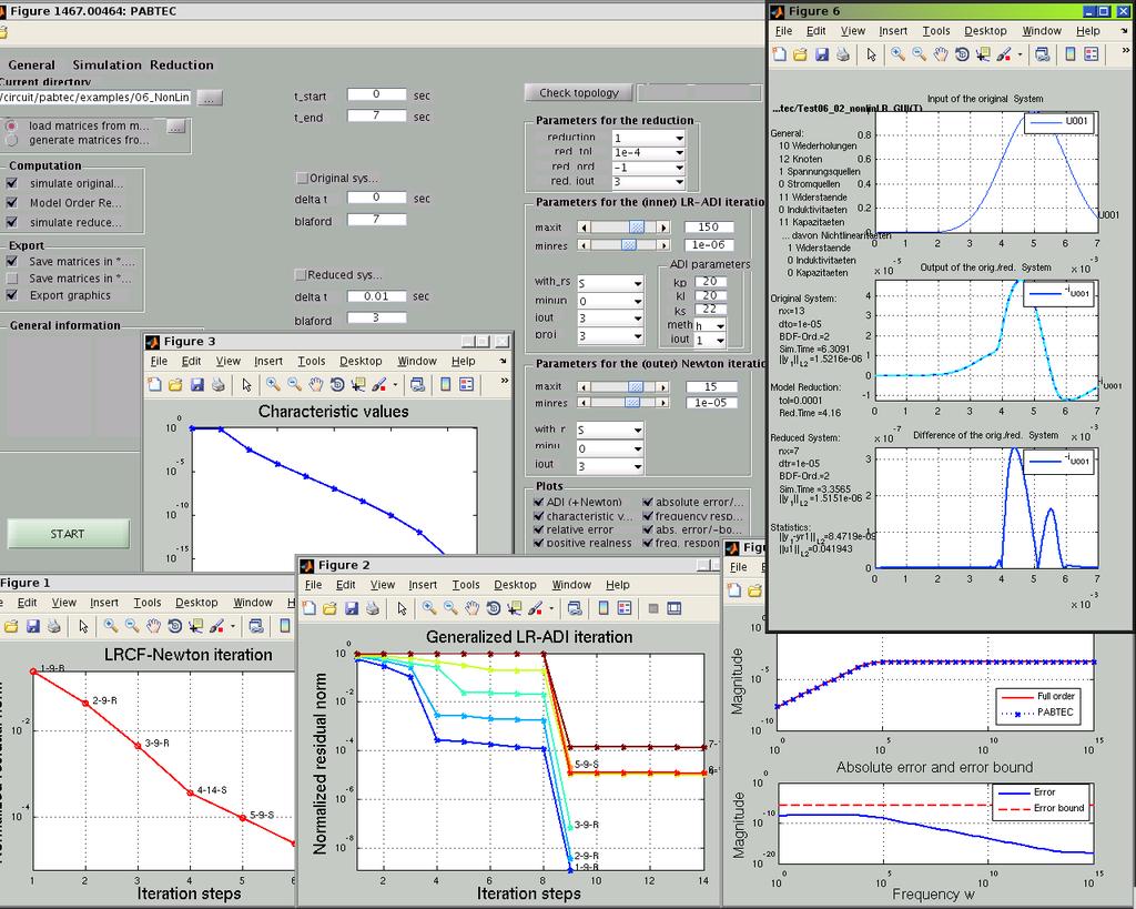
43 MATLAB-Toolbox: PABTEC

44 Contents: Introduction, Motivation Model equations for electrical circuits with nonlinear elements Model order reduction Software package: PABTEC Numerical tests Summary

45 Example 1 - Problem n = 53 u R g(.) R R R Input: voltage source 1 5 uv C C C C C t 52 nodes 1 voltage source 51 linear capacities 1 output 5 linear resistors 1 diode State dimension of the model equations n = 53 Simulation is done for t [s,.7s] using BDF method of order 2 with fixed stepsize of length The computations are done with MATLAB.

46 Example 1 - Simulation results n = 53 u R g(.) R R R Input: voltage source 1 5 uv C C C C C t 6 x Output: negative current of the voltage source orig. system red. system 6 x Output: negative current of the voltage source orig. system red. system i V 2 i V 2 i V t x 1 5 Error of the output with prescribed tolerance t i V t x 1 6 Error of the output with prescribed tolerance t

47 Example 1 - Efficiency n = 53 Dimension of the red. system vs. prescribed tolerance 16 Error of the output vs. prescribed tolerance Speedup vs. prescribed tolerance dimension of the red. system error 1 6 speedup prescribed tolerance prescribed tolerance prescribed tolerance dimension of the original system simulation time for the original system 6772s 6772s 6772s 6772s prescribed tolerance for the model reduction 1e-2 1e-3 1e-4 1e-5 time for the model reduction 7s 8s 27s 46s dimension of the reduced system simulation time for the reduced system 76s 18s 118s 146s obtained error of the output of the red. system 6.2e-6 8.7e-7 2.5e-7 2.9e-7 speedup

48 Example 1 - Problem n = 153 u R g(.) R R R Input: voltage source 1 5 uv C C C C C t 152 nodes 1 voltage source 151 linear capacities 1 output 15 linear resistors 1 diode State dimension of the model equations n = 153 Simulation is done for t [s,.7s] using BDF method of order 2 with fixed stepsize of length The computations are done with MATLAB.

49 Example 1 - Simulation results n = 153 u R g(.) R R R Input: voltage source 1 5 uv C C C C C t 6 x Output: negative current of the voltage source orig. system red. system 6 x Output: negative current of the voltage source orig. system red. system i V 2 i V 2 i V t x 1 5 Error of the output with prescribed tolerance t i V t x 1 6 Error of the output with prescribed tolerance t

50 Example 1 - Efficiency n = 153 Dimension of the red. system vs. prescribed tolerance 19 Error of the output vs. prescribed tolerance Speedup vs. prescribed tolerance dimension of the red. system prescribed tolerance error prescribed tolerance speedup prescribed tolerance dimension of the original system simulation time for the original system 2412s 2412s 2412s 2412s prescribed tolerance for the model reduction 1e-2 1e-3 1e-4 1e-5 time for the model reduction 15s 24s 42s 61s dimension of the reduced system simulation time for the reduced system 82s 11s 122s 155s obtained error of the output of the red. system 7.e-6 6.2e-7 2.e-7 4.2e-7 speedup

51 Example 2 - Problem L 3 R2 L 6 R2 L 3N R2 R N 2 3N 1 3N+1 C R1 C R1 C L uv C 2C N*C g(.) LN(.) u Input: voltage source t 31 nodes 1 voltage source 2 linear capacities 1 output 199 linear resistors 1 diode 991 linear inductors 1 nonlinear inductors State dimension of the model equations n = 43 Simulation is done for t [s,.5s] using BDF method of order 2 with fixed stepsize of length The computations are done with MATLAB.

52 Example 2 - Simulation results L 3 R2 L 6 R2 L 3N R2 R N 2 3N 1 3N+1 C R1 C R1 C L uv C 2C N*C g(.) LN(.) u Input: voltage source t x 1 3 Output: negative current of the voltage source x 1 3 Output: negative current of the voltage source 15 orig. system red. system 15 orig. system red. system i V 1 i V t x 1 Error of the output t x 1 Error of the output i V t i V t

53 Example 2 - Efficiency Dimension of the red. system vs. prescribed tolerance Error of the output vs. prescribed tolerance 1 3 Speedup vs. prescribed tolerance 32 dimension of the red. system error speedup prescribed tolerance prescribed tolerance prescribed tolerance dimension of the original system simulation time for the original system 4557s 4557s 4557s 4557s prescribed tolerance for the model reduction 1e-3 1e-5 1e-7 1e-9 time for the model reduction 92s 822s 834s 9s dimension of the reduced system simulation time for the reduced system 43s 67s 125s 277s obtained error of the output of the red. system 1.6e-4 4.4e e-6 1.9e-6 speedup

54 Contents: Introduction, Motivation Model equations for electrical circuits with nonlinear elements Model order reduction Software package: PABTEC Numerical tests Summary

55 Summary We developed a model order reduction approach for the model equations of nonlinear circuits.

56 Summary We developed a model order reduction approach for the model equations of nonlinear circuits. The developed model reduction technique bases on... decoupling of linear and nonlinear subcircuits model reduction of the remained linear part recoupling of the reduced linear subcircuit with the unchanged nonlinear subcircuit

57 Summary We developed a model order reduction approach for the model equations of nonlinear circuits. The developed model reduction technique bases on... decoupling of linear and nonlinear subcircuits model reduction of the remained linear part recoupling of the reduced linear subcircuit with the unchanged nonlinear subcircuit The efficency and applicability of the proposed model reduction approach was demonstrated on several numerical examples.

Announcement MODRED 21 Workshop: MODRED 21 MODEL REDUCTION FOR COMPLEX DYNAMICAL SYSTEMS System Reduction for Nanoscale IC Design December 2-4, 21 TU Berlin, Germany Invited speakers: Michel S.

58 Announcement MODRED 21 Workshop: MODRED 21 MODEL REDUCTION FOR COMPLEX DYNAMICAL SYSTEMS System Reduction for Nanoscale IC Design December 2-4, 21 TU Berlin, Germany Invited speakers: Michel S. Nakhla (Carleton University, Ottawa) Joel R. Phillips (Cadence Berkeley Laboratories, San Jose) Timo Reis (TU Hamburg-Harburg) Important date: Registration: November 1, 21

59 Thank you for your attantion.

Model order reduction of electrical circuits with nonlinear elements

Model order reduction of electrical circuits with nonlinear elements Andreas Steinbrecher and Tatjana Stykel 1 Introduction The efficient and robust numerical simulation of electrical circuits plays a