Capacitor of capacitance C; Their schematic representations are shown in Figure below.

Transcription

1 UNIT 1 Basic Circuit Concepts In modern life, circuits are everywhere. Without circuits, you wouldn't have indoor lights. Without circuits, you wouldn't have the computer you're using to watch this lesson. Without circuits, you wouldn't have anything that is powered by electricity. A circuit is a series of electrical components or devices connected together in a complete loop, allowing electric current in the form of charged electrons to flow through it and power the components. There are practically an unlimited number of types of components that could go into a circuit, including batteries, bulbs, resistors, inductors, switches, capacitors, buzzers, diodes, temperature controls called thermistors, light sensors, and many others. CIRCUIT ELEMENTS The most commonly encountered linear one-ports are the Inductor of inductance L, Resistor of resistance R & Capacitor of capacitance C; Their schematic representations are shown in Figure below. One-port elements-- (a) an inductor of inductance, (b) a resistor of resistance R & (c) a capacitor of capacitance C. The equations relating voltage and current in the three one-ports, as well as their associated impedances are as follows: Inductor Resistor Capacitor (2.6) (2.7) (2.8) Each of these circuit elements is passive as long as its element value (L, C or R) is positive; the inductor and capacitor are easily shown to be lossless as well. The inductor and capacitor are examples of reactive circuits elements--all power instantaneously absorbed by either one will be stored and eventually be returned to the network to which it is connected. The resistor is passive, but not lossless. In addition to the one-ports mentioned above, we can also define the short - circuit, opencircuit, current source and voltage source (see Figure below) by:

2 Short-circuit Open-circuit Voltage source Current source Other one-ports-- (a) short-circuit, (b) open-circuit, (c) voltage source and (d) current source. Dots adjacent to the sources indicate polarity. The impedances of the short- and open-circuit one-ports are zero and infinity, respectively. Both are lossless. Kirchhoff s Law Kirchhoff's circuit laws are two equalities that deal with the current and potential difference (commonly known as voltage) in the lumped element model of electrical circuits. Kirchhoff s First Law The Current Law, (KCL) Kirchhoff s Current Law or KCL, states that the total current or charge entering a junction or node is exactly equal to the charge leaving the node as it has no other place to go except to leave, as no charge is lost within the node. In other words the algebraic sum of ALL the currents entering and leaving a node must be equal to zero, I (exiting) + I (entering) = 0. This idea by Kirchhoff is commonly known as the Conservation of Charge. Kirchhoff s Current Law Here, the 3 currents entering the node, I1, I2 and I3 are all positive in value and the 2 currents leaving the node, I4 and I5 are negative in value. Then this means we can also rewrite the equation as; I1 + I2 + I3 I4 I5 = 0 The term Node in an electrical circuit generally refers to a connection or junction of two or more current carrying paths or elements such as cables and components. Also for current to flow either in or out of a node a closed circuit path must exist. We can use Kirchhoff s current law when analysing parallel circuits.

3 Kirchhoff s Voltage Law: Starting at any point in the loop continue in the same direction noting the direction of all the voltage drops, either positive or negative, and returning back to the same starting point. It is important to maintain the same direction either clockwise or anti-clockwise or the final voltage sum will not be equal to zero. We can use Kirchhoff s voltage law when analysing series circuits. When analysing either DC circuits or AC circuits using Kirchhoff s Circuit Laws a number of definitions and terminologies are used to describe the parts of the circuit being analysed such as: node, paths, branches, loops and meshes. These terms are used frequently in circuit analysis so it is important to understand them. R, C, and L Elements and their V and I relationships We deal with three essential elements in circuit analysis: Resistance R Capacitance C Inductance L Their V and I relationships are summarized below.

4 Resistance is a static element in the sense V (t) versus I (t) relationship is instantaneous. For example, V (t) at time t = 2 seconds simply depends only on I (t) at t = 2 seconds and nothing else. This implies that the resistance does not know what happened in the past, in other words it does not store any energy unlike other elements C and L as we see soon. Unlike in the case of resistance, for a capacitance the V (t) versus I (t) relationship and vice versa at any time t depends on the past as they involve diff erentials and integrals. This implies that the capacitance is a dynamic element. What happened in the past influences the present behaviour. As we shall see soon, capacitance stores energy. Once again, unlike in the case of resistance, for an inductance the V (t) versus I (t) relationship and vice versa at any time t depends on the past as they involve diff erentials and integrals. This implies that the inductance is a dynamic element. What happened in the past influences the present behaviour. As we shall see soon, inductance stores energy Independent and Dependent Sources There are two principal types of source, namely voltage source and current source. Sources can be either independent or dependent upon some other quantities. An independent voltage source maintains a voltage (fixed or varying with time) which is not affected by any other quantity. Similarly an independent current source maintains a current (fixed or time-varying) which is unaffected by any other quantity. The usual symbols are shown in figure. Figure: Symbols for independent sources

5 Some voltage (current) sources have their voltage (current) values varying with some other variables. They are called dependent voltage (current) sources or controlled voltage (current) sources, and their usual symbols are shown in figure below. Remarks - It is not possible to force an independent voltage source to take up a voltage which is different from its defined value. Likewise, it is not possible to force an independent current source to take up a current which is different from its defined value. Two particular examples are short-circuiting an independent voltage source and open-circuiting an independent current source. Both are not permitted. Figure: Symbols for dependent sources. Variables in brackets are the controlling variables whose values affect the value of the source. Simple Resistive Circuits Resistors in Series Resistors in Parallel The Voltage-Divider and Current-Divider Circuits Voltage Division and Current Division Measuring Voltage and Current Resistors in Series

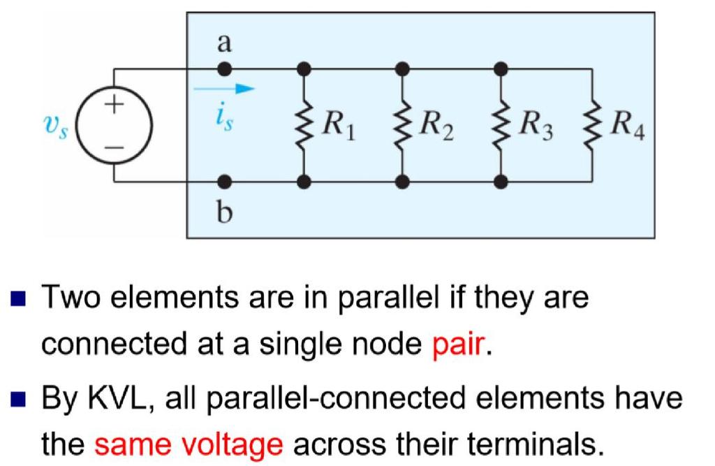
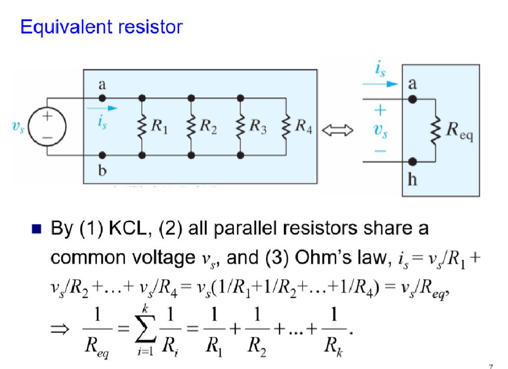
6 Resistors in Parallel

7 The Voltage-Divider

8 Current-Divider Circuits

9 Mesh Current Method The Mesh Current Method, also known as the Loop Current Method, is quite similar to the Branch Current method in that it uses simultaneous equations, Kirchhoff s Voltage Law, and Ohm s Law to determine unknown currents in a network. It differs from the Branch Current method in that it does not use Kirchhoff s Current Law, and it is usually able to solve a circuit with less unknown variables and less simultaneous equations, which is especially nice if you re forced to solve without a calculator. Mesh Current, conventional method Let s see how this method works on the same example problem: The first step in the Mesh Current method is to identify loops within the circuit encompassing all components. In our example circuit, the loop formed by B1, R1, and R2 will be the first while the loop formed by B2, R2, and R3 will be the second. The strangest part of the Mesh Current method is envisioning circulating currents in each of the loops. In fact, this method gets its name from the idea of these currents meshing together between loops like sets of spinning gears:

10 The choice of each current s direction is entirely arbitrary, just as in the Branch Current method, but the resulting equations are easier to solve if the currents are going the same direction through intersecting components (note how currents I1 and I2 are both going up through resistor R2, where they mesh, or intersect). If the assumed direction of a mesh current is wrong, the answer for that current will have a negative value. The next step is to label all voltage drop polarities across resistors according to the assumed directions of the mesh currents. Remember that the upstream end of a resistor will always be negative, and the downstream end of a resistor positive with respect to each other, since electrons are negatively charged. The battery polarities, of course, are dictated by their symbol orientations in the diagram, and may or may not agree with the resistor polarities (assumed current directions): Using Kirchhoff s Voltage Law, we can now step around each of these loops, generating equations representative of the component voltage drops and polarities. As with the Branch Current method, we will denote a resistor s voltage drop as the product of the resistance (in ohms) and its respective mesh current (that quantity being unknown at this point). Where two currents mesh together, we will write that term in the equation with resistor current being the sum of the two meshing currents. Tracing the left loop of the circuit, starting from the upper-left corner and moving counter-clockwise (the choice of starting points and directions is ultimately irrelevant), counting polarity as if we had a voltmeter in hand, red lead on the point ahead and black lead on the point behind, we get this equation: Notice that the middle term of the equation uses the sum of mesh currents I1 and I2 as the current through resistor R2. This is because mesh currents I1 and I2 are going the same direction through R2, and thus complement each other. Distributing the coefficient of 2 to the I1 and I2 terms, and then combining I1 terms in the equation, we can simplify as such: At this time we have one equation with two unknowns. To be able to solve for two unknown mesh currents, we must have two equations. If we trace the other loop of the circuit, we can obtain another KVL equation and have enough data to solve for the two currents. Creature of habit that I am, I ll start at the upper-left hand corner of the right loop and trace counterclockwise:

11 Simplifying the equation as before, we end up with: Now, with two equations, we can use one of several methods to mathematically solve for the unknown currents I1 and I2: Knowing that these solutions are values for mesh currents, not branch currents, we must go back to our diagram to see how they fit together to give currents through all components: The solution of -1 amp for I2 means that our initially assumed direction of current was incorrect. In actuality, I2 is flowing in a counter-clockwise direction at a value of (positive) 1 amp: This change of current direction from what was first assumed will alter the polarity of the voltage drops across R2 and R3 due to current I2. From here, we can say that the current through R1 is 5 amps, with the voltage drop across R1 being the product of current and resistance (E=IR), 20 volts (positive on the left and negative on the right). Also, we can safely say that the current through R3 is 1 amp, with a voltage drop of 1 volt (E=IR), positive on the left and negative on the right. But what is happening at R2? Mesh current I1 is going up through R2, while mesh current I2 is going down through R2. To determine the actual current through R2, we must see how mesh currents I1 and I2 interact (in this case they re in opposition), and algebraically add them to arrive at a final

12 value. Since I1 is going up at 5 amps, and I2 is going down at 1 amp, the real current through R2 must be a value of 4 amps, going up: A current of 4 amps through R2 s resistance of 2 Ω gives us a voltage drop of 8 volts (E=IR), positive on the top and negative on the bottom. The primary advantage of Mesh Current analysis is that it generally allows for the solution of a large network with fewer unknown values and fewer simultaneous equations. Our example problem took three equations to solve the Branch Current method and only two equations using the Mesh Current method. This advantage is much greater as networks increase in complexity: To solve this network using Branch Currents, we d have to establish five variables to account for each and every unique current in the circuit (I1 through I5). This would require five equations for solution, in the form of two KCL equations and three KVL equations (two equations for KCL at the nodes, and three equations for KVL in each loop):

13 I suppose if you have nothing better to do with your time than to solve for five unknown variables with five equations, you might not mind using the Branch Current method of analysis for this circuit. For those of us who have better things to do with our time, the Mesh Current method is a whole lot easier, requiring only three unknowns and three equations to solve: Less equations to work with is a decided advantage, especially when performing simultaneous equation solution by hand (without a calculator). Another type of circuit that lends itself well to Mesh Current is the unbalanced Wheatstone Bridge. Take this circuit, for example: The directions of these mesh currents, of course, is arbitrary. However, two mesh currents is not enough in this circuit, because neither I 1 nor I 2 goes through the battery. So, we must add a third mesh current, I 3 :

14 Here, I have chosen I 3 to loop from the bottom side of the battery, through R 4, through R 1, and back to the top side of the battery. This is not the only path I could have chosen for I 3, but it seems the simplest. Now, we must label the resistor voltage drop polarities, following each of the assumed currents directions: Notice something very important here: at resistor R 4, the polarities for the respective mesh currents do not agree. This is because those mesh currents (I 2 and I 3 ) are going through R 4 in different directions. This does not preclude the use of the Mesh Current method of analysis, but it does complicate it a bit. Though later, we will show how to avoid the R 4 current clash. (See Example below) Generating a KVL equation for the top loop of the bridge, starting from the top node and tracing in a clockwise direction:

15 In this equation, we represent the common directions of currents by their sums through common resistors. For example, resistor R 3, with a value of 100 Ω, has its voltage drop represented in the above KVL equation by the expression 100(I 1 + I 2 ), since both currents I 1 and I 2 go through R 3 from right to left. The same may be said for resistor R 1, with its voltage drop expression shown as 150(I 1 + I 3 ), since both I 1 and I 3 go from bottom to top through that resistor, and thus work together to generate its voltage drop. Generating a KVL equation for the bottom loop of the bridge will not be so easy, since we have two currents going against each other through resistor R 4. Here is how I do it (starting at the right-hand node, and tracing counter-clockwise): Note how the second term in the equation s original form has resistor R 4 s value of 300 Ω multiplied by the difference between I 2 and I 3 (I 2 - I 3 ). This is how we represent the combined effect of two mesh currents going in opposite directions through the same component. Choosing the appropriate mathematical signs is very important here: 300(I 2 - I 3 ) does not mean the same thing as 300(I 3 - I 2 ). I chose to write 300(I 2 - I 3 ) because I was thinking first of I 2 s effect (creating a positive voltage drop, measuring with an imaginary voltmeter across R 4, red lead on the bottom and black lead on the top), and secondarily of I 3 s effect (creating a negative voltage drop, red lead on the bottom and black lead on the top). If I had thought in terms of I 3 s effect first and I 2 s effect secondarily, holding my imaginary voltmeter leads in the same positions (red on bottom and black on top), the expression would have been -300(I 3 - I 2 ). Note that this expression is mathematically equivalent to the first one: +300(I 2 - I 3 ). Well, that takes care of two equations, but I still need a third equation to complete my simultaneous equation set of three variables, three equations. This third equation must also include the battery s voltage, which up to this point does not appear in either two of the previous KVL equations. To generate this equation, I will trace a loop again with my imaginary voltmeter starting from the battery s bottom (negative) terminal, stepping clockwise (again, the direction in which I step is arbitrary, and does not need to be the same as the direction of the mesh current in that loop):

16 Solving for I 1, I 2, and I 3 using whatever simultaneous equation method we prefer: Node Voltage Method The node voltage method of analysis solves for unknown voltages at circuit nodes in terms of a system of KCL equations. This analysis looks strange because it involves replacing voltage sources with equivalent current sources. Also, resistor values in ohms are replaced by equivalent conductance in Siemens, G = 1/R. The Siemens (S) is the unit of conductance, having replaced the mho unit. In any event S = Ω-1. And S = mho (obsolete). We start with a circuit having conventional voltage sources. A common node E 0 is chosen as a reference point. The node voltages E 1 and E 2 are calculated with respect to this point. A voltage source in series with a resistance must be replaced by an equivalent current source in parallel with the resistance. We will write KCL equations for each node. The right hand side of the equation is the value of the current source feeding the node.

17 Replacing voltage sources and associated series resistors with equivalent current sources and parallel resistors yields the modified circuit. Substitute resistor conductances in siemens for resistance in ohms. The parallel conductances (resistors) may be combined by addition of the conductances. Though, we will not redraw the circuit. The circuit is ready for application of the node voltage method. Deriving a general node voltage method, we write a pair of KCL equations in terms of unknown node voltages V1 and V2 this one time. We do this to illustrate a pattern for writing equations by inspection. The coefficients of the last pair of equations above have been rearranged to show a pattern. The sum of conductances connected to the first node is the positive coefficient of the first voltage in equation (1). The sum of conductances connected to the second node is the positive coefficient of the second voltage in equation (2). The other coefficients are negative, representing conductances between nodes. For both equations, the right hand side is equal to the respective current source connected to the node. This pattern allows us to quickly write the equations by inspection. This leads to a set of rules for the node voltage method of analysis. Node voltage rules: Convert voltage sources in series with a resistor to an equivalent current source with the resistor in parallel. Change resistor values to conductances. Select a reference node (E0) Assign unknown voltages (E1) (E2)... (EN) to remaining nodes.

18 Write a KCL equation for each node 1,2,... N. The positive coefficient of the first voltage in the first equation is the sum of conductances connected to the node. The coefficient for the second voltage in the second equation is the sum of conductances connected to that node. Repeat for coefficient of third voltage, third equation, and other equations. These coefficients fall on a diagonal. All other coefficients for all equations are negative, representing conductances between nodes. The first equation, second coefficient is the conductance from node 1 to node 2, the third coefficient is the conductance from node 1 to node 3. Fill in negative coefficients for other equations. The right hand side of the equations is the current source connected to the respective nodes. Solve system of equations for unknown node voltages.

19 UNIT 2 SINUSOIDAL STEADY STATE ANALYSIS Phasor A vector that represents a sinusoidally varying quantity, as a current or voltage, by means of a line rotating about a point in a plane, the magnitude of the quantity being proportional to the length of the line and the phase of the quantity being equal to the angle between the line and a reference line is known as Phasor. Euler's formula indicates that sinusoids can be represented mathematically as the sum of two complex-valued functions: Or as the real part of one of the functions: The function is the analytic representation of Sinusoidal Steady State Response Concepts of Impedance and Admittance In electrical engineering, sinusoidal forcing functions are particularly important. The alternating sinusoidal current of power frequencies (50 Hz, 60 Hz) is extensively used for producing, transmitting and utilizing electric energy in industry and in the home. Highfrequency sinusoids (of kilohertz, megahertz and gigahertz) are used as carrier signals for communication purposes. Sinusoids are in abundance in nature, as, for example, in the movement of a pendulum, in the bouncing of a ball, and in the vibrations of strings and membranes.

20 In electrical engineering, sinusoidal forcing functions are particularly important. The alternating sinusoidal current of power frequencies (50 Hz, 60 Hz) is extensively used for producing, transmitting and utilizing electric energy in industry and in the home. Highfrequency sinusoids (of kilohertz, megahertz and gigahertz) are used as carrier signals for communication purposes. Sinusoids are in abundance in nature, as, for example, in the movement of a pendulum, in the bouncing of a ball, and in the vibrations of strings and membranes. Historically, in the late 1800s the primary use of electricity was in direct current (d.c.) operating systems. The first big power system in New York and New Jersey was Edison's direct current system. However, it became clear that some of the disadvantages of d.c. had hindered the development of the widespread use of electric power. Thus, the use of alternating current (a.c.) and its 'competition' with d.c. began. It is evident that the a.c. system won this competition. The main advantage of the a.c. over d.c. is the efficiency of transmission. Alternating voltage can be transformed to high voltages, thus reducing the loss on the transmission line. If a line has a wire resistance R and the power transmitted is proportional to V], the power lost in the lines is ]2 R. Thus, if the transmitted voltage could be set at a high level (typically today up to 765 kv) which allows the current to be kept low, the line losses would be minimized. Transformers, which are used to step up and step down the a.c. voltage, also are very efficient and require practically no maintenance. Typically, in a power station the output voltage of the a.c. generators (also sometimes called alternators) is in the range: kv. It is then stepped up to hundreds of kilovolts for long-distance transmission, and then it is stepped down for use in factories and homes. Another advantage of a.c. is the convenience of producing electric power. In practice, a.c. generators are easier to build than d.c. machines for two main reasons: (a) high-voltage high-current armature windings are on the stator (instead of on the rotor as in d.c. generators); (b) the voltage induced in the stator is naturally oscillatory and almost sinusoidal. Finally, with three-phase a.c. circuits (see Chapter 4) it is easy to create a rotating magnetic field and to produce cheap and reliable induction motors-the main drive in industry. It is also cheaper to build threephase transmission lines and uses less conductive material (copper and aluminum), since only three wires are needed instead of six to transmit the same power. Sinusoidal forcing functions are relatively easily analyzed. In the sinusoidal steady-state behavior of linear time-invariant circuits, when they are driven by one or more sinusoidal sources at some angular frequency OJ, all currents and voltages are sinusoidal at the same frequency OJ. (Note that steady-state behavior sets in after all 'transients' have died down.)

21 Analysis of simple circuit Example 1 Consider Figure 8.1 with the following Parameters: V1=15V V2=7V R1=2Ω R2=20Ω R3=10Ω R4=5Ω R5=2Ω R6=2Ω Find current through R3 using Mesh Analysis method. Solution: Figure 8.2: Currents in loops This is the same example we solved in Exercise 7. We can see that there are three closed paths (loops) where we can apply KVL in, Loop 1, 2 and 3 as shown in figure 8.2 We can now apply KVL arround the loops remembering Passive Convention when defining Currents and voltages. KVL around abca loop: Therefore, KVL around acda loop: Therefore KVL around bdcb loop: Therefore

22 Now we can create a matrix with the above equations as follows: The following matrix is the above with values substituted: Solving determinants of: Matrix A: General matrix A from KVL equations Matrix A1 : General Matrix A with Column 1 substituted by Matrix A2 : General Matrix A with Column 2 substituted by Matrix A3 : General Matrix A with Column 3 substituted by Now we can use the solved determinants to arrive at solutions for Mesh Currents I1, I2 & I3 as follows:

23 Now we can solve for the current through R3 as follows: POWER AND POWER FACTOR In an AC circuit, the voltage and current waveforms are sinusoidal so their amplitudes are constantly changing over time. Since we know that power is voltage times the current (P = V*I), maximum power will occur when the two voltage and current waveforms are lined up with each other. That is, their peaks and zero crossover points occur at the same time. When this happens the two waveforms are said to be in-phase. The three main components in an AC circuit which can affect the relationship between the voltage and current waveforms, and therefore their phase difference, by defining the total impedance of the circuit are the resistor, the capacitor and the inductor. The impedance, (Z) of an AC circuit is equivalent to the resistance calculated in DC circuits, with impedance given in ohms. For AC circuits, impedance is generally defined as the ratio of the voltage and current phasor s produced by a circuit component. Phasor s are straight lines drawn in such a way as to represents a voltage or current amplitude by its length and its phase difference with respect to other phasor lines by its angular position relative to the other phasor s. AC circuits contain both resistance and reactance that are combined together to give a total impedance (Z) that limits current flow around the circuit. But an AC circuits impedance is not equal to the algebraic sum of the resistive and reactive ohmic values as a pure resistance and pure reactance are 90 o out-of-phase with each other. But we can use this 90 o phase difference as the sides of a right angled triangle, called an impedance triangle, with the impedance being the hypotenuse as determined by Pythagoras theorem. This geometric relationship between resistance, reactance and impedance can be represented visually by the use of an impedance triangle as shown.

24 Note that impedance, which is the vector sum of the resistance and reactance, has not only a magnitude (Z) but it also has a phase angle (θ), which represents the phase difference between the resistance and the reactance. Also note that the triangle will change shape due to variations in reactance, (X) as the frequency changes. Of course, resistance (R) will always remain constant. We can take this idea one step further by converting the impedance triangle into a power triangle representing the three elements of power in an AC circuit. Ohms Law tells us that in a DC circuit, power (P), in watts, is equal to the current squared (I 2 ) times the resistance (R). So we can multiply the three sides of our impedance triangle above by I 2 to obtain the corresponding power triangle as: Real Power P = I 2 R Watts, (W) Reactive Power Q = I 2 X Volt-amperes Reactive, (VAr) Apparent Power S = I 2 Z Volt-amperes, (VA) Real Power in AC Circuits Real power P, also known as true or active power, performs the real work within an electrical circuit. Real power, measured in watts, defines the power consumed by the resistive part of a circuit. Then real power, P in an AC circuit is the same as power, P in a DC circuit. So just like DC circuits, it is always calculated as I 2 R, where R is the total resistive component of the circuit. As resistances do not produce any phasor difference (phase shift) between voltage and current waveforms, all the useful power is delivered directly to the resistance and converted to heat, light and work. Then the power consumed by a resistance is real power which is fundamentally the circuits average power. To find the corresponding value of the real power the rms voltage and current values are multiplied by the cosine of the phase angle, θ as shown. Real Power P = I 2 R = V*I*cos(θ) Watts, (W) But as their is no phase difference between the voltage and the current in a resistive circuit, the phase shift between the two waveforms will be zero (0). Then: Real Power in an AC Circuit Where real power (P) is in watts, voltage (V) is in rms volts and current (I) is in rms amperes. Then real power is the I 2 R resistive element measured in watts, which is what you read on your utility energy meter and has units in Watts (W), Kilowatts (kw), and Megawatts (MW). Note that real power, P is always positive.

25 Reactive Power in AC Circuits Reactive power Q, (sometimes called wattless power) is the power consumed in an AC circuit that does not perform any useful work but has a big effect on the phase shift between the voltage and current waveforms. Reactive power is linked to the reactance produced by inductors and capacitors and counteracts the effects of real power. Reactive power does not exist in DC circuits. Unlike real power (P) which does all the work, reactive power (Q) takes power away from a circuit due to the creation and reduction of both inductive magnetic fields and capacitive electrostatic fields, thereby making it harder for the true power to supply power directly to a circuit or load. The power stored by an inductor in its magnetic field tries to control the current, while the power stored by a capacitors electrostatic field tries to control the voltage. The result is that capacitors generate reactive power and inductors consume reactive power. This means that they both consume and return power to the source so none of the real power is consumed. To find reactive power, the RMS voltage and current values are multiplied by the sine of the phase angle, θ as shown. Reactive Power Q = I 2 X = V*I*sin(θ) volt-amperes reactive, (VAr s) As there is a 90 o phase difference between the voltage and the current waveforms in a pure reactance (either inductive or capacitive), multiplying VI by sinθ gives a vertical component that is 90 o out-of-phase with each other, so: Reactive Power in an AC Circuit Where reactive power (Q) is in volt-amperes reactive, voltage (V) is in rms volts and current (I) is in rms amperes. Then reactive power represents the product of volts and amperes that are 90 o out-of-phase with each other, but in general, there can be any phase angle, θ between the voltage and the current. Thus reactive power is the I 2 X reactive element that has units in volt-amperes reactive (VAr), Kilovolt-amperes reactive (kvar), and Megavolt-amperes reactive (MVAr).

26 Apparent Power in AC Circuits We have seen above that real power is dissipated by resistance and that reactive power is supplied to a reactance. As a result of this the current and voltage waveforms are not in-phase due to the difference between a circuits resistive and reactive components. Then there is a mathematical relationship between the real power (P), and the reactive power (Q), called the complex power. The product of the rms voltage, V applied to an AC circuit and the rms current, I flowing into that circuit is called the volt-ampere product (VA) given the symbol S and whose magnitude is known generally as apparent power. This complex Power is not equal to the algebraic sum of the real and reactive powers added together, but is instead the vector sum of P and Q given in volt-amps (VA). It is complex power that is represented by the power triangle. The rms value of the volt-ampere product is known more commonly as the apparent power as, apparently this is the total power consumed by a circuit even though the real power that does the work is a lot less. As apparent power is made up of two parts, the resistive power which is the in-phase power or real power in watts and the reactive power which is the out-of-phase power in voltamperes, we can show the vector addition of these two power components in the form of a power triangle. A power triangle has four parts: P, Q, S and θ. The three elements which make up power in an AC circuit can be represented graphically by the three sides of a right-angled triangle, in much the same way as the previous impedance triangle. The horizontal (adjacent) side represents the circuits real power (P), the vertical (opposite) side represents the circuits reactive power (Q) and the hypotenuse represents the resulting apparent power (S), of the power triangle as shown. Power Triangle of an AC Circuit Where: P is the I 2 R or Real power that performs work measured in watts, W Q is the I 2 X or Reactive power measured in volt-amperes reactive, VAr S is the I 2 Z or Apparent power measured in volt-amperes, VA θ is the phase angle in degrees. The larger the phase angle, the greater the reactive power Cosθ = P/S = W/VA = power factor, p.f. Sinθ = Q/S = VAr/VA Tanθ = Q/P = VAr/W The power factor is calculated as the ratio of the real power to the apparent power because this ratio equals cosθ. Power Factor in AC Circuits Power factor, cosθ, is an important part of an AC circuit that can also be expressed in terms of circuit impedance or circuit power. Power factor is defined as the ratio of real power (P) to apparent power (S), and is generally expressed as either a decimal value, for example 0.95, or as a percentage: 95%.

27 Power factor defines the phase angle between the current and voltage waveforms, were I and V are the magnitudes of rms values of the current and voltage. Note that it does not matter whether the phase angle is the difference of the current with respect to the voltage, or the voltage with respect to the current. The mathematical relationship is given as: Power Factor of an AC Circuit: We said previously that in a pure resistive circuit, the current and voltage waveforms are inphase with each other so the real power consumed is the same as the apparent power as the phase difference is zero degrees (0 o ). So the power factor will be: Power Factor, pf = cos 0 o = 1.0 That is the number of watts consumed is the same as the number of volt-amperes consumed producing a power factor of 1.0, or 100%. In this case it is referred to a unity power factor. We also said above that in a purely reactive circuit, the current and voltage waveforms are out-of-phase with each other by 90 o. As the phase difference is ninety degrees (90 o ), the power factor will be: Power Factor, pf = cos 90 o = 0 That is the number of watts consumed is zero but there is still a voltage and current supplying the reactive load. Clearly then reducing the reactive VAr component of the power triangle will cause θ to reduce improving the power factor towards one, unity. It is also desirable to have a high power factor as this makes the most efficient use of the circuit delivering current to a load. Then we can write the relationship between the real power, the apparent power and the circuits power factor as: An inductive circuit where the current lags the voltage (ELI) is said to have a lagging power factor, and a capacitive circuit where the current leads the voltage (ICE) is said to have a leading power factor.

28 Power Triangle Example 1 A wound coil that has an inductance of 180mH and a resistance of 35Ω is connected to a 100V 50Hz supply. Calculate: a) the impedance of the coil, b) the current, c) the power factor, and d) the apparent power consumed. Also draw the resulting power triangle for the above coil. Data given: R = 35Ω, L = 180mH, V = 100V and ƒ = 50Hz. (a) Impedance (Z) of the coil: (b) Current (I) consumed by the coil: (c) The power factor and phase angle, θ: (d) Apparent power (S) consumed by the coil:

29 (e) Power triangle for the coil: As the power triangle relationships of this simple example demonstrates, at or 52.63% power factor, the coil requires 150 VA of power to produce 79 Watts of useful work. In other words, at 52.63% power factor, the coil takes about 88% more current to do the same work, which is a lot of wasted current. Adding a power factor correction capacitor (for this example a 32.3uF) across the coil, in order to increase the power factor to over 0.95, or 95%, would greatly reduce the reactive power consumed by the coil as these capacitors act as reactive current generators, thus reducing the total amount of current consumed. Power Triangle and Power Factor Summary We have seen here that the three elements of electrical power, Real Power, Reactive Power and Apparent Power in an AC circuit can be represented by the three sides of a triangle called

30 a Power Triangle. As these three elements are represented by a right-angled triangle, their relationship can be defined as: S 2 = P 2 + Q 2, where P is the real power in watts (W), Q is the reactive power in volt-amperes reactive (VAr) and S is the apparent power in volt-amperes (VA). We have also seen that in an AC circuit, the quantity cosθ is called the power factor. The power factor of an AC circuit is defined as the ratio of the real power (W) consumed by a circuit to the apparent power (VA) consumed by the same circuit. This therefore gives us: Power Factor = Real Power/Apparent Power, or pf = W/VA. Then the cosine of the resulting angle between the current and voltage is the power factor. Generally power factor is expressed as a percentage, for example 95%, but can also be expressed as a decimal value, for example When the power factor equals 1.0 (unity) or 100%, that is when the real power consumed equals the circuits apparent power, the phase angle between the current and the voltage is 0 o as: cos-1(1.0) = 0 o. When the power factor equals zero (0), the phase angle between the current and the voltage will be 90 o as: cos-1(0) = 90 o. In this case the actual power consumed by the AC circuit is zero regardless of the circuit current. In practical AC circuits, the power factor can be anywhere between 0 and 1.0 depending on the passive components within the connected load. For an inductive-resistive load or circuit (which is most often the case) the power factor will be lagging. In a capacitive-resistive circuit the power factor will be leading. Then an AC circuit can be defined to have a unity, lagging, or leading power factor. A poor power factor with a value towards zero (0) will consume wasted power reducing the efficiency of the circuit, while a circuit or load with a power factor closer to one (1.0) or unity (100%), will be more efficient. This is because a a circuit or load with a low power factor requires more current than the same circuit or load with a power factor closer to 1.0 (unity). Solution of three phase balanced circuits and three phase unbalanced circuits Requirements of a Balanced 3-Phase Set Following are the requirements that must be satisified in order for a set of 3 sinusoidal variables (usually voltages or currents) to be a "balanced 3-phase set" All 3 variables have the same amplitude All 3 variables have the same frequency All 3 variables are 120o in phase In terms of the time domain, a set of balance 3-phase voltages has the following general form. va = Vm cos ( t + ) vb = Vm cos ( t o ) vc = Vm cos ( t o ) = Vm cos ( t o ) Notice that we have assumed (and will continue to assume) positive (abc) phase sequence, i.e., phase "b" follows 120o behind "a" & phase "c" follows 120o behind phase "b" Figure 1 below illustrates the balanced 3-phase voltages in time domain.

31 Figure 1: Balanced 3-Phase Variables in Time Domain In terms of phasors, we write the same balanced set as follows. Note that the phasors are in rms, as will be assumed throughout this course. V a = V m m V b = V m o V c = V m o = V m +120 o Thus, V b = V a (1-120 o ), and V c = V a ( o ) Figure 2 below illustrates the balanced 3-phase phasors graphically. Requirements of a Balanced 3-Phase Circuit Following are the requirements that must be satisified in order for a 3-phase system or circuit to be balanced All 3 sources are reprensented by a set of balanced 3-phase variables All loads are 3-phase with equal impedances Line impedances are equal in all 3 phases Having a balanced circuit allows for simplified analysis of the 3-phase circuit. In fact, if the circuit is balanced, we can solve for the voltages, currents, and powers, etc. in one phase using circuit analysis. The values of the corresponding variables in the other two phases can be found using some basic equations. This type of solution is accomplished using a "one-line diagram", which will be discussed later. If the circuit is not balanced, all three phases should be analyzed in detail. Figure 3 illustrates a balanced 3-phase circuit and some of the naming conventions to be used in this course Following are the requirements that must be satisified in order for a 3-phase system or circuit to be balanced 1. All 3 sources are reprensented by a set of balanced 3-phase variables 2. All loads are 3-phase with equal impedances

32 3. Line impedances are equal in all 3 phases Having a balanced circuit allows for simplified analysis of the 3-phase circuit. In fact, if the circuit is balanced, we can solve for the voltages, currents, and powers, etc. in one phase using circuit analysis. The values of the corresponding variables in the other two phases can be found using some basic equations. This type of solution is accomplished using a "one-line diagram", which will be discussed later. If the circuit is not balanced, all three phases should be analyzed in detail. Figure 3 illustrates a balanced 3-phase circuit and some of the naming conventions to be used in this course A Balanced 3-Phase Circuit Power measurement in three phase circuits In this method we have two types of connections Star connection of loads Delta connection of loads. When the star connected load, the diagram is shown in below- For star connected load clearly the reading of wattmeter one is product phase current and voltage difference (V 2 -V 3 ). Similarly the reading of wattmeter two is the product of phase current and the voltage difference (V 2 -V 3 ). Thus the total power of the circuit is sum of the reading of both the wattmeter. Mathematically we can write

33 but we have, hence putting the value of. We get total power as. When delta connected load, the diagram is shown in below The reading of wattmeter one can be written as and reading of wattmeter two is But, hence expression for total power will reduce to. Measurement of Three Phase Power by One Wattmeter Method Limitation of this method is that it cannot be applied on unbalanced load. So under this condition we have. Diagram is shown below: Two switches are given which are marked as 1-3 and 1-2, by closing the switch 1-3 we get reading of wattmeter as Similarly the reading of wattmeter when switch 1-2 is closed is

34 UNIT 3 Superposition Theorem Superposition theorem is one of those strokes of genius that takes a complex subject and simplifies it in a way that makes perfect sense. A theorem like Millman s certainly works well, but it is not quite obvious why it works so well. Superposition, on the other hand, is obvious. The strategy used in the Superposition Theorem is to eliminate all but one source of power within a network at a time, using series/parallel analysis to determine voltage drops (and/or currents) within the modified network for each power source separately. Then, once voltage drops and/or currents have been determined for each power source working separately, the values are all superimposed on top of each other (added algebraically) to find the actual voltage drops/currents with all sources active. Let s look at our example circuit again and apply Superposition Theorem to it: Since we have two sources of power in this circuit, we will have to calculate two sets of values for voltage drops and/or currents, one for the circuit with only the 28 volt battery in effect and one for the circuit with only the 7 volt battery in effect: When re-drawing the circuit for series/parallel analysis with one source, all other voltage sources are replaced by wires (shorts), and all current sources with open circuits (breaks). Since we only have voltage sources (batteries) in our example circuit, we will replace every inactive source during analysis with a wire.

35 Analyzing the circuit with only the 28 volt battery, we obtain the following values for voltage and current: Analyzing the circuit with only the 7 volt battery, we obtain another set of values for voltage and current: When superimposing these values of voltage and current, we have to be very careful to consider polarity (voltage drop) and direction (electron flow), as the values have to be added algebraically.

36 Currents add up algebraically as well, and can either be superimposed as done with the resistor voltage drops, or simply calculated from the final voltage drops and respective resistances (I=E/R). Either way, the answers will be the same. Here I will show the superposition method applied to current: Once again applying these superimposed figures to our circuit: Thevenin s Theorem Thevenin s Theorem states that it is possible to simplify any linear circuit, no matter how complex, to an equivalent circuit with just a single voltage source and series resistance connected to a load. The qualification of linear is identical to that found in the Superposition Theorem, where all the underlying equations must be linear (no exponents or roots). If we re dealing with passive components (such as resistors, and later, inductors and capacitors), this is true. However, there are some components (especially certain gasdischarge and semiconductor components) which are nonlinear: that is, their opposition to current changes with voltage and/or current. As such, we would call circuits containing these types of components, nonlinear circuits. Thevenin s Theorem is especially useful in analyzing power systems and other circuits where one particular resistor in the circuit (called the load resistor) is subject to change, and re-calculation of the circuit is necessary with each trial value of load resistance, to determine voltage across it and current through it. Let s take another look at our example circuit:

37 Let s suppose that we decide to designate R2 as the load resistor in this circuit. We already have four methods of analysis at our disposal (Branch Current, Mesh Current, Millman s Theorem, and Superposition Theorem) to use in determining voltage across R2 and current through R2, but each of these methods are time-consuming. Imagine repeating any of these methods over and over again to find what would happen if the load resistance changed (changing load resistance is very common in power systems, as multiple loads get switched on and off as needed. the total resistance of their parallel connections changing depending on how many are connected at a time). This could potentially involve a lot of work! Thevenin s Theorem makes this easy by temporarily removing the load resistance from the original circuit and reducing what s left to an equivalent circuit composed of a single voltage source and series resistance. The load resistance can then be re-connected to this Thevenin equivalent circuit and calculations carried out as if the whole network were nothing but a simple series circuit:.. after Thevenin conversion.. The Thevenin Equivalent Circuit is the electrical equivalent of B1, R1, R3, and B2 as seen from the two points where our load resistor (R2) connects. The Thevenin equivalent circuit, if correctly derived, will behave exactly the same as the original circuit formed by B1, R1, R3, and B2. In other words, the load resistor (R2) voltage and current should be exactly the same for the same value of load resistance in the two circuits. The load resistor R2 cannot tell the difference between the original network of B1, R1, R3, and B2, and the Thevenin equivalent circuit of EThevenin, and RThevenin, provided that the values for EThevenin and RThevenin have been calculated correctly. The advantage in performing the Thevenin conversion to the simpler circuit, of course, is that it makes load voltage and load current so much easier to solve than in the original

38 network. Calculating the equivalent Thevenin source voltage and series resistance is actually quite easy. First, the chosen load resistor is removed from the original circuit, replaced with a break (open circuit): Next, the voltage between the two points where the load resistor used to be attached is determined. Use whatever analysis methods are at your disposal to do this. In this case, the original circuit with the load resistor removed is nothing more than a simple series circuit with opposing batteries, and so we can determine the voltage across the open load terminals by applying the rules of series circuits, Ohm s Law, and Kirchhoff s Voltage Law: The voltage between the two load connection points can be figured from the one of the battery s voltage and one of the resistor s voltage drops, and comes out to 11.2 volts. This is our Thevenin voltage (E Thevenin ) in the equivalent circuit: To find the Thevenin series resistance for our equivalent circuit, we need to take the original circuit (with the load resistor still removed), remove the power sources (in the same style as

39 we did with the Superposition Theorem: voltage sources replaced with wires and current sources replaced with breaks), and figure the resistance from one load terminal to the other: With the removal of the two batteries, the total resistance measured at this location is equal to R 1 and R 3 in parallel: 0.8 Ω. This is our Thevenin resistance (R Thevenin ) for the equivalent circuit: With the load resistor (2 Ω) attached between the connection points, we can determine voltage across it and current through it as though the whole network were nothing more than a simple series circuit: Notice that the voltage and current figures for R 2 (8 volts, 4 amps) are identical to those found using other methods of analysis. Also notice that the voltage and current figures for the Thevenin series resistance and the Thevenin source (total) do not apply to any component in the original, complex circuit. Thevenin s Theorem is only useful for determining what happens to a single resistor in a network: the load. The advantage, of course, is that you can quickly determine what would happen to that single resistor if it were of a value other than 2 Ω without having to go through a lot of analysis again. Just plug in that other value for the load resistor into the Thevenin equivalent circuit and a little bit of series circuit calculation will give you the result. Norton s Theorem Norton s Theorem states that it is possible to simplify any linear circuit, no matter how complex, to an equivalent circuit with just a single current source and parallel

40 resistance connected to a load. Just as with Thevenin s Theorem, the qualification of linear is identical to that found in the Superposition Theorem: all underlying equations must be linear (no exponents or roots). Contrasting our original example circuit against the Norton equivalent: it looks something like this:... after Norton conversion... Remember that a current source is a component whose job is to provide a constant amount of current, outputting as much or as little voltage necessary to maintain that constant current. As with Thevenin s Theorem, everything in the original circuit except the load resistance has been reduced to an equivalent circuit that is simpler to analyze. Also similar to Thevenin s Theorem are the steps used in Norton s Theorem to calculate the Norton source current (I Norton ) and Norton resistance (R Norton ). As before, the first step is to identify the load resistance and remove it from the original circuit:

41 Then, to find the Norton current (for the current source in the Norton equivalent circuit), place a direct wire (short) connection between the load points and determine the resultant current. Note that this step is exactly opposite the respective step in Thevenin s Theorem, where we replaced the load resistor with a break (open circuit): With zero voltage dropped between the load resistor connection points, the current through R 1 is strictly a function of B 1 s voltage and R 1 s resistance: 7 amps (I=E/R). Likewise, the current through R 3 is now strictly a function of B 2 s voltage and R 3 s resistance: 7 amps (I=E/R). The total current through the short between the load connection points is the sum of these two currents: 7 amps + 7 amps = 14 amps. This figure of 14 amps becomes the Norton source current (I Norton ) in our equivalent circuit: Remember, the arrow notation for a current source points in the direction opposite that of electron flow. Again, apologies for the confusion. For better or for worse, this is standard electronic symbol notation. Blame Mr. Franklin again!

42 To calculate the Norton resistance (R Norton ), we do the exact same thing as we did for calculating Thevenin resistance (R Thevenin ): take the original circuit (with the load resistor still removed), remove the power sources (in the same style as we did with the Superposition Theorem: voltage sources replaced with wires and current sources replaced with breaks), and figure total resistance from one load connection point to the other: Now our Norton equivalent circuit looks like this: If we re-connect our original load resistance of 2 Ω, we can analyze the Norton circuit as a simple parallel arrangement: As with the Thevenin equivalent circuit, the only useful information from this analysis is the voltage and current values for R 2 ; the rest of the information is irrelevant to the original circuit. However, the same advantages seen with Thevenin s Theorem apply to Norton s as well: if we wish to analyze load resistor voltage and current over several different values of load resistance, we can use the Norton equivalent circuit again and again, applying nothing more complex than simple parallel circuit analysis to determine what s happening with each trial load.

43 Maximum Power Transfer Theorem The Maximum Power Transfer Theorem is not so much a means of analysis as it is an aid to system design. Simply stated, the maximum amount of power will be dissipated by a load resistance when that load resistance is equal to the Thevenin/Norton resistance of the network supplying the power. If the load resistance is lower or higher than the Thevenin/Norton resistance of the source network, its dissipated power will be less than maximum. This is essentially what is aimed for in radio transmitter design, where the antenna or transmission line impedance is matched to final power amplifier impedance for maximum radio frequency power output. Impedance, the overall opposition to AC and DC current, is very similar to resistance, and must be equal between source and load for the greatest amount of power to be transferred to the load. A load impedance that is too high will result in low power output. A load impedance that is too low will not only result in low power output, but possibly overheating of the amplifier due to the power dissipated in its internal (Thevenin or Norton) impedance. Taking our Thevenin equivalent example circuit, the Maximum Power Transfer Theorem tells us that the load resistance resulting in greatest power dissipation is equal in value to the Thevenin resistance (in this case, 0.8 Ω): With this value of load resistance, the dissipated power will be 39.2 watts: If we were to try a lower value for the load resistance (0.5 Ω instead of 0.8 Ω, for example), our power dissipated by the load resistance would decrease:

44 Power dissipation increased for both the Thevenin resistance and the total circuit, but it decreased for the load resistor. Likewise, if we increase the load resistance (1.1 Ω instead of 0.8 Ω, for example), power dissipation will also be less than it was at 0.8 Ω exactly: If you were designing a circuit for maximum power dissipation at the load resistance, this theorem would be very useful. Having reduced a network down to a Thevenin voltage and resistance (or Norton current and resistance), you simply set the load resistance equal to that Thevenin or Norton equivalent (or vice versa) to ensure maximum power dissipation at the load. Practical applications of this might include radio transmitter final amplifier stage design (seeking to maximize power delivered to the antenna or transmission line), a grid tied inverter loading a solar array, or electric vehicle design (seeking to maximize power delivered to drive motor). The Maximum Power Transfer Theorem is not: Maximum power transfer does not coincide with maximum efficiency. Application of The Maximum Power Transfer theorem to AC power distribution will not result in maximum or even high efficiency. The goal of high efficiency is more important for AC power distribution, which dictates a relatively low generator impedance compared to load impedance. Similar to AC power distribution, high fidelity audio amplifiers are designed for a relatively low output impedance and a relatively high speaker load impedance. As a ratio, output impdance : load impedance is known as damping factor, typically in the range of 100 to [rar] [dfd] Maximum power transfer does not coincide with the goal of lowest noise. For example, the low-level radio frequency amplifier between the antenna and a radio receiver is often designed for lowest possible noise. This often requires a mismatch of the amplifier input impedance to the antenna as compared with that dictated by the maximum power transfer theorem.

45 UNIT 4 TRANSIENT RESPONSE FOR DC CIRCUITS TRANSIENT RESPONSE OF RL CIRCUITS: So far we have considered dc resistive network in which currents and voltages were independent of time. More specifically, Voltage (cause input) and current (effect output) responses displayed simultaneously except for a constant multiplicative factor (VR). Two basic passive elements namely, inductor and capacitor are introduced in the dc network. Automatically, the question will arise whether or not the methods developed in lesson-3 to lesson-8 for resistive circuit analysis are still valid. The voltage/current relationship for these two passive elements are defined by the derivative (voltage across the inductor Our problem is to study the growth of current in the circuit through two stages, namely; (i) dc transient response (ii) steady state response of the system D.C Transients: The behavior of the current and the voltage in the circuit switch is closed until it reaches its final value is called dc transient response of the concerned circuit. The response of a circuit (containing resistances, inductances, capacitors and switches) due to sudden application of voltage or current is called transient response. The most common instance of a transient response in a circuit occurs when a switch is turned on or off a rather common event in an electric circuit.

46 Growth or Rise of current in R-L circuit To find the current expression (response) for the circuit shown in fig. 10.6(a), we can write the KVL equation around the circuit The table shows how the current i(t) builds up in a R-L circuit.

47

48 Consider network shown in fig. the switch k is moved from position 1 to 2 at reference time t = 0. Now before switching take place, the capacitor C is fully charged to V volts and it discharges through resistance R. As time passes, charge and hence voltage across capacitor i.e. Vc decreases gradually and hence discharge current also decreases gradually from maximum to zero exponentially. After switching has taken place, applying kirchoff s voltage law, Where VR is voltage across resistor and VC is voltage across capacitor.

49 Above equation is linear, homogenous first order differential equation. Hence rearranging we have, Integrating both sides of above equation we have Now at t = 0, VC =V which is initial condition, substituting in equation we have, Where Q is total charge on capacitor Similarly at any instant, VC = q/c where q is instantaneous charge. Thus charge behaves similarly to voltage across capacitor. Now discharging current i is given by

50 but VR = VC when there is no source in circuit. The above expression is nothing but discharge current of capacitor. The variation of this current with respect to time is shown in fig. This shows that the current is exponentially decaying. At point P on the graph. The current value is (0.368) times its maximum value. The characteristics of decay are determined by values R and C, which are 2 parameters of network. For this network, after the instant t = 0, there is no driving voltage source in circuit, hence it is called undriven RC circuit. TRANSIENT RESPONSE OF RC CIRCUITS Ideal and real capacitors: An ideal capacitor has an infinite dielectric resistance and plates (made of metals) that have zero resistance. However, an ideal capacitor does not exist as all dielectrics have some leakage current and all capacitor plates have some resistance. A capacitor s of how much charge (current) it will allow to leak through the dielectric medium. Ideally, a charged capacitor is not supposed to allow leaking any current through the dielectric medium and also assumed not to dissipate any power loss in capacitor plates resistance. Under this situation, the model as shown in fig (a) represents the ideal capacitor. However, all real or practical capacitor leaks current to some extend due to leakage resistance of dielectric medium. This leakage resistance can be visualized as a resistance connected in parallel with the capacitor and power loss in capacitor plates can be realized with a resistance connected in series with capacitor. The model of a real capacitor is shown in fig. Let us consider a simple series RC circuit shown in fig (a) is connected through a switch S to a constant voltage source.

51 The switch S is closed at time t=0 It is assumed that the capacitor is initially charged with a voltage and the current flowing through the circuit at any instant of time after closing the switch is Current decay in source free series RL circuit: - At t = 0-,, switch k is kept at position a for very long time. Thus, the network is in steady state. Initial current through inductor is given as, Because current through inductor can not change instantaneously Assume that at t = 0 switch k is moved to position 'b'. Applying KVL, Rearranging the terms in above equation by separating variables Integrating both sides with respect to corresponding variables Where k is constant of integration. To find- k : Form equation 1, at t=0, i=i0 Substituting the values in equation 3

52 Substituting value of k from equation 4 in fig. shows variation of current i with respect to time From the graph, H is clear that current is exponentially decaying. At point P on graph. The current value is (0.363) times its maximum value. The characteristics of decay are determined by values R and L which are two parameters of network. The voltage across inductor is given by

53 TRANSIENT RESPONSE OF RLC CIRCUITS In the preceding lesson, our discussion focused extensively on dc circuits having resistances with either inductor () or capacitor () (i.e., single storage element) but not both. Dynamic response of such first order system has been studied and discussed in detail. The presence of resistance, inductance, and capacitance in the dc circuit introduces at least a second order differential equation or by two simultaneous coupled linear first order differential equations. We shall see in next section that the complexity of analysis of second order circuits increases significantly when compared with that encountered with first order circuits. Initial conditions for the circuit variables and their derivatives play an important role and this is very crucial to analyze a second order dynamic system. Response of a series R-L-C circuit Consider a series RLcircuit as shown in fig.11.1, and it is excited with a dc voltage source C sv. Applying around the closed path for, The current through the capacitor can be written as Substituting the current expression in eq.(11.1) and rearranging the terms,

54 The above equation is a 2nd-order linear differential equation and the parameters associated with the differential equation are constant with time. The complete solution of the above differential equation has two components; the transient response and the steady state response. Mathematically, one can write the complete solution as Since the system is linear, the nature of steady state response is same as that of forcing function (input voltage) and it is given by a constant value. Now, the first part of the total response is completely dies out with time while and it is defined as a transient or natural response of the system. The natural or transient response (see Appendix in Lesson-10) of second order differential equation can be obtained from the homogeneous equation (i.e., from force free system) that is expressed by and solving the roots of this equation (11.5) on that associated with transient part of the complete solution (eq.11.3) and they are given below. The roots of the characteristic equation are classified in three groups depending upon the values of the parameters,,rland of the circuit Case-A (overdamped response): That the roots are distinct with negative real parts. Under this situation, the natural or transient part of the complete solution is written as and each term of the above expression decays exponentially and ultimately reduces to zero as and it is termed as overdamped response of input free system. A system that is overdamped responds slowly to any change in excitation. It may be noted that the exponential term

55 t 11tAeαtakes longer time to decay its value to zero than the term21taeα. One can introduce a factorξ that provides an information about the speed of system response and it is defined by damping ratio RLC Circuit: Consider a circuit in which R, L, and C are connected in series with each other across ac supply as shown in fig. The ac supply is given by, V = Vm sin wt The circuit draws a current I. Due to that different voltage drops are, 1. Voltage drop across Resistance R is VR = IR 2. Voltage drop across Inductance L is VL = IXL 3. Voltage drop across Capacitance C is Vc = IXc The characteristics of three drops are, (i) VR is in phase with current I

56 (ii) VL leads I by 900 (iii) Vc lags I by 900 According to krichoff s laws Steps to draw phasor diagram: 1. Take current I as reference 2. VR is in phase with current I 3. VL leads current by Vc lags current by obtain resultant of VL and Vc. Both VL and Vc are in phase opposition (1800 out of phase) 6. Add that with VRby law of parallelogram to get supply voltage. The phasor diagram depends on the condition of magnitude of VL and Vc which ultimately depends on values of XL and Xc. Let us consider different cases: Case(i): XL > Xc When X L > Xc Also VL > Vc (or) IXL > IXc So, resultant of VL and Vc will directed towards VL i.e. leading current I. Hence I lags V i.e. current I will lags the resultant of VL and Vc i.e. (V L - Vc). The circuit is said to be inductive in nature. From voltage triangle, If, V = Vm Sin wt ; i = Im Sin (wt - ф ) i.e I lags V by angle ф Case(ii): XL < Xc When XL < Xc Also VL < Vc (or) IXL < IXc Hence the resultant of VL and Vc will directed towards Vc i.e current is said to be capacitive in nature Form voltage triangle i.e I lags V by angle ф Case(iii): XL = Xc When XL = Xc Also VL = Vc (or) IXL = IXc

57 So VL and Vc cancel each other and the resultant is zero. So V = VR in such a case, the circuit is purely resistive in nature. Impedance: In general for RLC series circuit impedance is given by, Z = R + j X X = XL Xc = Total reactance of the circuit If XL > Xc ; X is positive & circuit is Inductive If XL < Xc ; X is negative & circuit is Capacitive If XL = Xc ; X =0 & circuit is purely Resistive Tan фl - =Xc[(X) R] Cos ф = [R Z] Z = 2 +(X L(R-Xc ) 2) Impedance triangle: In both cases R = Z Cos ф X = Z Sin ф Power and power triangle: The average power consumed by circuit is, Pavg = (Average power consumed by R) + (Average power consumed by L) + (Average power consumed by C) Pavg = Power taken by R = I2R = I(IR) = VI V = V Cos ф P = VI Cos ф Thus, for any condition, XL > Xc or XL < Xc General power can be expressed as P = Voltage x Component in phase with voltage Power triangle: S = Apparent power = I2Z = VI P = Real or True power = VI Cos ф = Active po Q = Reactive power = VI Sin ф

58 UNIT 5 RESONANCE AND COUPLED CIRCUITS Resonance in Series-Parallel Circuits In simple reactive circuits with little or no resistance, the effects of radically altered impedance will manifest at the resonance frequency predicted by the equation given earlier. In a parallel (tank) LC circuit, this means infinite impedance at resonance. In a series LC circuit, it means zero impedance at resonance: However, as soon as significant levels of resistance are introduced into most LC circuits, this simple calculation for resonance becomes invalid. We ll take a look at several LC circuits with added resistance, using the same values for capacitance and inductance as before: 10 µf and 100 mh, respectively. According to our simple equation, the resonant frequency should be Hz. Watch, though, where current reaches maximum or minimum in the following SPICE analyses: Parallel LC circuit with resistance in series with L.

59 Resistance in series with L produces minimum current at Hz instead of calculated Hz Parallel LC with resistance in serieis with C. Here, an extra resistor (R bogus ) (Figure below)is necessary to prevent SPICE from encountering trouble in analysis. SPICE can t handle an inductor connected directly in parallel with any voltage source or any other inductor, so the addition of a series resistor is necessary to break up the voltage source/inductor loop that would otherwise be formed. This resistor is chosen to be a very low value for minimum impact on the circuit s behavior. Resistance in series with C shifts minimum current from calculated Hz to roughly 180 Hz. Switching our attention to series LC circuits, (Figure below) we experiment with placing significant resistances in parallel with either L or C. In the following series circuit examples, a 1 Ω resistor (R 1 ) is placed in series with the inductor and capacitor to limit total current at resonance. The extra resistance inserted to influence resonant frequency effects is the 100 Ω resistor, R 2. The results are shown in (Figurebelow).

60 Series LC resonant circuit with resistance in parallel with L. Series resonant circuit with resistance in parallel with L shifts maximum current from Hz to roughly 180 Hz. And finally, a series LC circuit with the significant resistance in parallel with the capacitor. (Figure below) The shifted resonance is shown in (Figure below)

61 Series LC resonant circuit with rsistance in parallel with C. Resistance in parallel with C in series resonant circuit shifts curreent maximum from calculated Hz to about Hz. The tendency for added resistance to skew the point at which impedance reaches a maximum or minimum in an LC circuit is called antiresonance. The astute observer will notice a pattern between the four SPICE examples given above, in terms of how resistance affects the resonant peak of a circuit: Parallel ( tank ) LC circuit: R in series with L: resonant frequency shifted down R in series with C: resonant frequency shifted up Series LC circuit: R in parallel with L: resonant frequency shifted up R in parallel with C: resonant frequency shifted down Again, this illustrates the complementary nature of capacitors and inductors: how resistance in series with one creates an antiresonance effect equivalent to resistance in parallel with the other. If you look even closer to the four SPICE examples given, you ll see that the frequencies are shifted by the same amount, and that the shape of the complementary graphs are mirror-images of each other!

62 Antiresonance is an effect that resonant circuit designers must be aware of. The equations for determining antiresonance shift are complex, and will not be covered in this brief lesson. It should suffice the beginning student of electronics to understand that the effect exists, and what its general tendencies are. Added resistance in an LC circuit is no academic matter. While it is possible to manufacture capacitors with negligible unwanted resistances, inductors are typically plagued with substantial amounts of resistance due to the long lengths of wire used in their construction. What is more, the resistance of wire tends to increase as frequency goes up, due to a strange phenomenon known as the skin effect where AC current tends to be excluded from travel through the very center of a wire, thereby reducing the wire s effective cross-sectional area. Thus, inductors not only have resistance, but changing, frequency-dependent resistance at that. As if the resistance of an inductor s wire weren t enough to cause problems, we also have to contend with the core losses of iron-core inductors, which manifest themselves as added resistance in the circuit. Since iron is a conductor of electricity as well as a conductor of magnetic flux, changing flux produced by alternating current through the coil will tend to induce electric currents in the core itself (eddy currents). This effect can be thought of as though the iron core of the transformer were a sort of secondary transformer coil powering a resistive load: the less-than-perfect conductivity of the iron metal. This effects can be minimized with laminated cores, good core design and high-grade materials, but never completely eliminated. One notable exception to the rule of circuit resistance causing a resonant frequency shift is the case of series resistor-inductor-capacitor ( RLC ) circuits. So long as all components are connected in series with each other, the resonant frequency of the circuit will be unaffected by the resistance. (Figure below) The resulting plot is shown in (Figure below). Series LC with resistance in series. Maximum current at Hz once again!

63 Resistance in series resonant circuit leaves current maximum at calculated Hz, broadening the curve. Note that the peak of the current graph (Figure below) has not changed from the earlier series LC circuit (the one with the 1 Ω token resistance in it), even though the resistance is now 100 times greater. The only thing that has changed is the sharpness of the curve. Obviously, this circuit does not resonate as strongly as one with less series resistance (it is said to be less selective ), but at least it has the same natural frequency! It is noteworthy that antiresonance has the effect of dampening the oscillations of freerunning LC circuits such as tank circuits. In the beginning of this chapter we saw how a capacitor and inductor connected directly together would act something like a pendulum, exchanging voltage and current peaks just like a pendulum exchanges kinetic and potential energy. In a perfect tank circuit (no resistance), this oscillation would continue forever, just as a frictionless pendulum would continue to swing at its resonant frequency forever. But frictionless machines are difficult to find in the real world, and so are lossless tank circuits. Energy lost through resistance (or inductor core losses or radiated electromagnetic waves or...) in a tank circuit will cause the oscillations to decay in amplitude until they are no more. If enough energy losses are present in a tank circuit, it will fail to resonate at all. Antiresonance s dampening effect is more than just a curiosity: it can be used quite effectively to eliminate unwanted oscillations in circuits containing stray inductances and/or capacitances, as almost all circuits do. Take note of the following L/R time delay circuit: (Figure below) L/R time delay circuit The idea of this circuit is simple: to charge the inductor when the switch is closed. The rate of inductor charging will be set by the ratio L/R, which is the time constant of the circuit in seconds. However, if you were to build such a circuit, you might find unexpected oscillations (AC) of voltage across the inductor when the switch is closed. (Figure below)

64 Why is this? There s no capacitor in the circuit, so how can we have resonant oscillation with just an inductor, resistor, and battery? Inductor ringing due to resonance with stray capacitance. All inductors contain a certain amount of stray capacitance due to turn-to-turn and turn-tocore insulation gaps. Also, the placement of circuit conductors may create stray capacitance. While clean circuit layout is important in eliminating much of this stray capacitance, there will always be some that you cannot eliminate. If this causes resonant problems (unwanted AC oscillations), added resistance may be a way to combat it. If resistor R is large enough, it will cause a condition of antiresonance, dissipating enough energy to prohibit the inductance and stray capacitance from sustaining oscillations for very long. Interestingly enough, the principle of employing resistance to eliminate unwanted resonance is one frequently used in the design of mechanical systems, where any moving object with mass is a potential resonator. A very common application of this is the use of shock absorbers in automobiles. Without shock absorbers, cars would bounce wildly at their resonant frequency after hitting any bump in the road. The shock absorber s job is to introduce a strong antiresonant effect by dissipating energy hydraulically (in the same way that a resistor dissipates energy electrically). Mutual Inductance Mutual Inductance is the ratio between induced Electro Motive Force across a coil to the rate of change of current of another adjacent coil in such a way that two coils are in possibility of flux linkage.mutual induction is a phenomenon when a coil gets induced in EMF across it due to rate of change current in adjacent coil in such a way that the flux of one coil current gets linkage of another coil. Mutual inductance is denoted as ( M ), it is called coefficient of Mutual Induction between two coils. Mutual inductance for two coils gives the same value when they are in mutual induction

65 with each other. Induction in one coil due to its own rate of change of current is called self inductance (L), but due to rate of change of current of adjacent coil it gives mutual inductance (M). From the above figure, first coil carries current i 1 and its self inductance is L 1. Along with its self inductance it has to face mutual induction due to rate of change of current i 2 in the second coil. Same case happens in the second coil also. Dot convention is used to mark the polarity of the mutual induction. Suppose two coils are placed nearby. Coil 1 carries I 1 current having N 1 number of turn. Now the flux density created by the coil 1 is B 1. Coil 2 with N 2 number of turn gets linked with this flux from coil 1. So flux linkage in coil 2 is N 2. φ 21 [φ 21 is called leakage flux in coil 2 due to coil 1]. Consider φ 21 is also changing with respect to time, so an EMF appears across coil 2. This EMF is called mutually induced EMF. Now it can be written from these equations, Again, coil 1 gets induced by flux from coil 2 due to current I2 in the coil 2.

66 In same manner it can be written that for coil 1. However, using the reciprocity theorem which combines Ampere s law and the Biot-Savart law, one may show that the constants are equal. i.e. M 12 = M 21 = M. M is the mutual inductance for both coil in Henry. The value of mutual inductance is a function of the selfinductances Suppose two coils are place nearby such that they are in mutual induction. L 1 and L 2 are co-efficient of self induction of them. M is the mutual inductance. Here, ƙ is called co-efficient of coupling and it is defined as the ratio of mutual inductance actually present between the two coils to the maximum possible value. If the flux due to first coil completely links with second coil, then ƙ = 1, then two coils are tightly coupled. Again if no linkage at all then ƙ = 0 and hence two coils are magnetically isolated. Merits and demerits of mutual inductance: Due to mutual inductance, transformer establishes its operating principle. But due to mutual inductance, in any circuit having inductors, has to face extra voltage drop. How to find out L eq in a circuit having mutual inductance with dot conventionsuppose two coils are in series with same place dot. Mutual inductance between them is positive. Suppose two coils are in series with opposite place dot.

67 mutual When a few numbers of inductors are in series with inductances. Self-Inductance Self-inductance is the ration between the induced Electro Motive Force (EMF) across a coil to the rate of change of current through this coil. Self-inductance is related term to selfinduction phenomenon. Because of self-induction self-inductance generates. Self-inductance or Co-efficient of Self-induction is denoted as L. Its unit is Henry (H). First we have to know what self-induction is. Self-induction is the phenomenon by which in a coil a change in electric current produces an induced Electro Motive Force across this coil itself. This induced Electro Motive Force (ε) across this coil is proportional to the current changing rate. The higher the rate of change in current, the higher the value of EMF. We can write that,

68 But the actual equation is The question is that why there is Minus (-) sign? This Induced EMF across this coil is always opposite to the direction of the rate of change of current as per Lenz s Law. When current (I) flows through a coil some electric flux produces inside the coil in the direction of the current flowing. At that moment of self induction phenomenon, the induced EMF generates to oppose this rate of change of current in that coil. So their values are same but sign differs. Look at the figure below. Take a closer look at a coil that is carrying current. The magnetic field forms concentric loops that surround the wire and join to form larger loops that surround the coil. When the current increases in one loop the expanding magnetic field will cut across some or all of the neighboring loops of wire, inducing a voltage in these loops. For the DC source, when the switch is ON, i.e. just at t = 0+, a current will flow from its zero value to a certain value and with respect to time there will be a rate of change in current

69 momentarily. This current produces magnetic flux lines (φ) through this coil. As current changes its value to zero to a certain value that s why magnetic flux (φ) get rate of change with respect to the time, i.e. Now apply Faraday's Law in this coil, Where, N is the number of turn of the coil and e is the induced EMF across this coil. Lenz's law states that an induced current due to induced EMF has a direction such that its magnetic field opposes the change in magnetic field that induced the current. As per Lenz s law we can write down this equation of induced voltage across the coil, Now, we can modify this equation to calculate the value of inductance of a coil. so, [B is the flux density i.e. B =φ/a, A is area of the coil], [N. φ or L.I is called magnetic flux Linkage and it is denoted by Ѱ] Again, H.l = N.I, where H is the magnetizing force due to which magnetic flux lines flow from south to north pole inside the coil, l is the effective length of the coil and r is the radius of the coil cross-sectional area. L is a geometric quantity; it depends only on the dimensions of the solenoid, and the number of turns in the solenoid. Furthermore, in a DC circuit when the switch is just closed, then only momentarily effect of selfinductance occurs in the coil. After then no effect of self inductance is in a coil. It is because of steady flow of unidirectional current through this coil after closing the operating switch after t = 0+. But in AC circuit, alternating effect of current always causes the self-induction in the coil and a certain value of this self-inductance gives the inductive reactance depending on the value of supply frequency. Generally in the electrical circuit the coils those are used are known as inductor having values of L 1, L 2, L 3 etc. when they are series combination then equivalent inductance of them is calculated as When they are in parallel, then