ADVANCES IN SIMULATION AND THERMOGRAPHY FOR HIGH FIELD MRI

Transcription

1 The Pennsylvania State University The Graduate School Department of Bioengineering ADVANCES IN SIMULATION AND THERMOGRAPHY FOR HIGH FIELD MRI A Dissertation in Bioengineering by Zhipeng Cao 2013 Zhipeng Cao Submitted in Partial Fulfillment of the Requirements for the Degree of Doctor of Philosophy August 2013

2 The dissertation of Zhipeng Cao was reviewed and approved* by the following: Qing X. Yang Professor of Bioengineering Dissertation Advisor Chair of Committee William J. Weiss Professor of Bioengineering Thomas Neuberger Assistant Professor of Bioengineering Jesse Barlow Professor of Computer Science and Engineering Christopher M. Collins Special Member Professor of Radiology, New York University Mark A. Griswold Special Member Professor of Radiology, Case Western Reserve University Cheng Dong Professor Head of the Department of Bioengineering *Signatures are on file in the Graduate School

3 iii ABSTRACT High field Magnetic resonance imaging (MRI) systems can benefit from increased signalto-noise ratio (SNR) but face challenges of decreased homogeneity in signal intensity across images and increased patient heating. Currently, engineering studies for high field MRI involve modeling of human subjects and RF coils and calculating the MR relevant electromagnetic fields, as well as collecting experimental MR data to validate the simulation prediction. Presented here is a computer-based MRI system simulator developed to solve the Bloch equation with consideration of accurate electromagnetic fields calculated with finite-difference-time-domain (FDTD) method. It is demonstrated that the MRI system simulator can simulate many realistic MR phenomena. It bridges the gap between field simulation and experimental MR imaging, and can potentially facilitate the validation of new ideas by MR researchers. By utilizing the system simulator and an FDTD solver, an analysis of high field MRI performance at up to 14 Tesla with current standard transmission and reception methods has been performed. It is found that for imaging of the human head, depending on the imaging sequence used high field MRI could have more-than-linear increase in SNR and less-than-quadratic increase in energy dissipation in the subject. Finally, in order to explore the possibility of patient-specific temperature monitoring to ensure safety due to increased power deposition at high field, a novel compressed sensing reconstruction technique is presented to improve the acquisition speed of proton resonance frequency shift thermography.

4 iv TABLE OF CONTENTS List of Figures... vi List of Tables... ix Acknowledgements... x Chapter 1 Background Knowledge of MRI Nuclear Magnetic Resonance Imaging with NMR: Magnetic Resonance Imaging Common MRI Sequences: Gradient Recalled Echo Sequence and Spin Echo Sequence... 7 Chapter 2 Introduction of High Field MRI Research High field MRI Overview: Benefits and Challenges Increase of Transmit and Receive Field Inhomogeneities with Static Magnetic Field Strengths Linear Increase of SNR with Static Magnetic Field Strengths Quadratic Increase of SAR with Static Magnetic Field Strengths Parallel Transmission and RF Safety Electromagnetic Field Calculation Proton Resonance Frequency Shift Thermometry Chapter 3 Bloch-based MRI System Simulator Considering Realistic Electromagnetic Fields for Calculation of Signal, Noise, and SAR Abstract Introduction Theory Methods Results Discussion Chapter 4 Numerical Evaluation of Signal Intensity Homogeneity, Signal-to-noise Ratio, and Specific Absorption Rate for Human Brain Imaging at 1.5, 3, 7, 10.5 and 14 Tesla based on Electromagnetic Field Calculation and Bloch Simulation Abstract Introduction Methods Results Discussion Conclusions Chapter 5 COmplex-difference COnstrained Reconstruction with Baseline (COCORB) for Fast PRF Thermometry based RF Heating Evaluation... 64

5 v 5.1 Abstract Introduction Background and Theory Method Results Discussion Conclusion References... 90

6 vi LIST OF FIGURES Figure 1-1. Pulse sequence diagram of a standard GRE sequence. The gradient lobe of PE and the first lobe of FE serve as the pre-phasing gradient. The second gradient lobe of FE serves as the frequency encoding gradient Figure 1-2. Illustration of the magnetization vectors at two different spatial locations during a gradient echo sequence Figure 1-3. K-space data acquisition trajectory of a GRE sequence. Dashed lines denote the effects of pre-phasing frequency encoding (FE) gradient and phase encoding (PE) gradient to move the data acquisition position to the edge of k-space. Solid lines denote the process of acquiring each line of k-space data with frequency gradient turned on Figure 1-4. Pulse sequence diagram of a standard SE sequence. The gradient lobe of PE and the first lobe of FE serve as the pre-phasing gradient. The second gradient lobe of FE serves as the frequency encoding gradient Figure 1-5. Illustration of the magnetization vectors at two different spatial locations during a spin echo sequence Figure 1-6. K-space data acquisition trajectory of a SE sequence. Dashed lines on the left denote the effects of pre-phasing frequency encoding (FE) gradient and phase encoding (PE) gradient to move the data acquisition position to the edge of k-space. Dashed lines on the right denote the effect of phase reversal due to 180 degree RF pulse. Solid lines denote the process of acquiring each line of k-space data with frequency gradient turned on Figure 2-1. Increase of transmit field inhomogeneities (left) with their resultant signal intensity inhomogeneities (middle), and power deposition in SAR with the increase of frequency of MRI (Collins and Smith, 2001a) Figure 2-2. Modeling a body array with a realistic human phantom in xfdtd Figure 3-1. Model of the human head phantom within an eight-channel transmit/receive coil Figure 3-2. Geometry of a phantom and a birdcage coil for SNR validation Figure 3-3. Simulated k-space (a) and MR images with different contrast types (b-d): (a) an example of simulated k-space data, (b) T 1 weighted image, (c) T 2 weighted image, (d) proton density weighted image Figure 3-4. Simulated MR images with ΔB 0 (a, b) and chemical shift (c) artifacts: image distortion and signal loss artifacts due to in-plane and through-plane B 0 inhomogeneity with (a) GRE-EPI, and (b) long TE GRE, and (c) chemical shift artifact in a simulated phantom consisted of oil surrounded by CSF

7 vii Figure 3-5. Stimulated echo train simulated with different signal calculation methods. In (a) stimulated echoes are labeled SE1 through SE5 and signal spikes corresponding to pulses are marked P1 through P3. Tracking spatial gradients of the magnetization vector (Eq. 10) combined with multiple magnetization vectors (MV) per voxel (d) allows for more accurate production of the expected echo train (a) than when gradient tracking is not performed (b), with same number of magnetization vectors Figure 3-6. Spin echo images simulated by various methods showing the least artifact from inaccurate representation of continuous spin distributions with both tracking of spatial gradients (Eq. 10) of the magnetization vector (MV) and using multiple inplane magnetization vectors per voxel. The required computation time are recorded on the lower right corner of each image Figure 3-7. Signal intensity distribution (top) and SAR distribution (bottom) due to eight channel parallel transmission with quadrature excitation (left) and RF shimming (right) Figure 3-8. Simulated GRAPPA reconstruction with various reduction factors (R=1, 2, 3, and 4) showing noise distribution consistent with expectations Figure 3-9. Experimental and simulated SNR distribution of a phantom imaged with a transmit/receive birdcage coil Figure 4-1. Schematic diagram of the design of multichannel transmit and receive array Figure 4-2. The simulated MR images with quadrature excitation and reception for different field strengths. Constant TR (500 ms) leads to more T 1 weighting at higher field strength Figure 4-3. The simulated MR images with RF shimming for transmission and uniform receive fields for reception on the simulated center slice. With TE equaling inverse of B 0 and TR equaling 3 times of T 1 of gray matter leads to similar signal loss and image contrasts at all field strengths Figure 4-4. The simulated MR images with RF shimming for transmission and uniform receive fields for reception on the simulated below-center slice. With TE equaling inverse of B 0 and TR equaling 3 times of T 1 of gray matter leads to similar signal loss and image contrasts at all field strengths Figure 4-5. The simulated MR images with RF shimming for transmission and realistic receive magnetic fields for reception on simulated center slice. With TE equaling inverse of B 0 and TR equaling 3 times of T 1 of gray matter leads to similar signal loss and image contrasts at all field strengths Figure 4-6. The simulated MR images with RF shimming for transmission and realistic receive magnetic fields for reception on simulated below-center slice. With TE equaling inverse of B 0 and TR equaling 3 times of T 1 of gray matter leads to similar signal loss and image contrasts at all field strengths

8 Figure 4-7. Trends of (a) brain average SNR with 2 ms and 10 ms TE, and (b) brain average SNR per square root of scan time with 2 ms and 10 ms TE, both with increase of B 0 field strengths. The TRs used equal 3 times the value of T 1 of gray matter of each field strengths Figure 4-8. Trends of (a) head-averaged energy deposition, and (b) head-averaged SAR, both with increase of B 0 field strengths. The TRs used equal 3 times the value of T 1 of gray matter of each field strengths Figure 4-9. Trends of (a) maximum 10g-energy deposition, and (b) maximum 10g-SAR deposition, both with increase of B 0 field strengths. The TRs used equal 3 times the value of T 1 of gray matter of each field strengths Figure 5-1. Heating setup with a dedicated heating coil placed below the forearm of a volunteer. The five imaged slices are shown as black lines Figure 5-2. Magnitude images (a), phase and masked PRF temperature change images (b) used in the simulation study. Post-heating and baseline images are denoted as u and u 0. Undersampling images are denoted with. The undersampling mask is shown in (a) Figure 5-3. PRF images with different magnitude image SNRs and from various reconstruction methods, with RMSEs listed on the lower right for the heated ROI Figure 5-4. Fully-sampled magnitude and phase images of the post-heating images, and their corresponding PRF temperature change images, complex difference magnitude images, and magnitude difference ratio images (in percent), all from the retrospective multi-slice in vivo forearm heating study Figure 5-5. Reconstruction results from a retrospectively undersampled k-space dataset for in vivo human forearm heating. Results here demonstrate improved accuracy and robustness of the proposed method by using various undersampling trajectories and reconstruction methods on different imaging slices. (a)~(e) corresponds to slices 1~5 in Figure Figure 5-6. Anatomical image from the beef heating study. The arrow shows the location (red) where a fiber optic temperature probe was inserted Figure 5-7. Reconstructed PRF images and their spatial error distributions with RMSE of different time frames from a 12-frame time series Figure 5-8. Evaluation of temporal consistency of the proposed reconstruction method by comparing with temperature probe reading and/or fully-sampled temperature change at different locations Figure 5-9. Reconstruction accuracy demonstration of the proposed method compared to variations of previously-published method with reconstructed temperature maps listed on the left, spatial error on the right, and RMSE at the bottom viii

9 ix LIST OF TABLES Table 4-1. Frequency-dependent T 2 * values (in ms) for different tissue types Table 4-2. Frequency-dependent T 1 values (in ms) for different tissue types Table 4-3. Frequency-dependent electric conductivity values (in S/m) for different tissue types Table 4-4. Frequency-dependent relative permittivity values for different tissue types

10 x ACKNOWLEDGEMENTS First and foremost, I would like to thank my mentor Dr. Christopher M. Collins, for his kind and visionary guidance through the years of my Ph.D study. Dr. Collins has been providing me lots of opportunities that I can never forget. I would also like to thank Dr. Mark A. Griswold for his great idea that led to some parts of the dissertation. I thank Dr. Qing X. Yang for his helpful discussions and sense of humor that made my research life more enjoyable. I greatly appreciate the help from Dr. William Weiss, Dr. Jesse Barlow, and Dr. Thomas Neuberger for being my committee members and sharing valuable suggestions. Among many coworkers that shared the hardship of research with me, I would like to thank Dr. Christopher T. Sica the first. Besides, Dr. Sukhoon Oh is a wonderful presenter, and Patti Miller is a great technologist that helped me with experiments. I have had the honor to work alongside many excellent people. Rahul Dewal, Dr. Chien-ping Kao, Dr. Yeun-chul Ryu, Wei Luo, and Sebastian Rupprecht have been among those with whom I have shared the lab. I would also like to thank the faculty and staff from the Penn State Hershey MRI lab and department of Bioengineering. Last but not least, I would like to thank my wife, Dai Liu, for her constant support and encouragement. Life as a researcher is filled with unpredictable ups and downs, and I have always been optimistic with the helps from every one of you.

11 Chapter 1 Background Knowledge of MRI

12 2 This section is intended to provide basic knowledge for the readers to appreciate the relevance of the work presented in this dissertation. Magnetic resonance imaging (MRI) is a modern medical imaging technology that evolved from the discovery of nuclear magnetic resonance (NMR). This chapter includes NMR physical principles, the engineering fundamentals to use NMR phenomena for imaging, and description of standard MR imaging sequences. 1.1 Nuclear Magnetic Resonance Nuclear magnetic resonance (NMR) is a physical phenomenon in which nuclei in a static magnetic field can interact with radiofrequency magnetic fields. The electromagnetic energy must be transmitted to and received from the nuclei at a specific resonance frequency which depends on the strength of the static magnetic field and the magnetic properties of the isotope of the atoms. Among many isotopes that have nuclear magnetic resonance effects, 1 H (single-proton hydrogen) is most commonly used in practice for clinical imaging, due to its simplicity in magnetic resonance physics, strong magnetic moment, high precessional frequency, and abundance in the human body. These 1 H nuclei ( spins ) can be thought of as charged particles that spin about the applied static magnetic field as their axes. The rotation of each nucleus produces a magnetic moment, m, along the nucleus's axis of rotation. At each spatial tissue location, ensembles of these magnetic moments are defined as three dimensional magnetization vectors, M. With classical physics representation, the NMR phenomenon of 1 H can be described by the magnetization vector evolution from the Bloch equation in the laboratory frame (Bloch, 1946). dm dt M M x y M z M 0 M B xˆ yˆ zˆ T2 T2 T1 (Eq. 1)

13 3 Here T 1 and T 2 are the longitudinal and transverse relaxation times respectively, B the applied static and radiofrequency magnetic fields, ρ 0 the density of 1 H ( per m 3 for water), γ the gyromagnetic ratio (for 1 H, γ = MHz/T), ћ the Planck s constant, k the Boltzmann constant, and T the tissue temperature. M 0 denotes the longitudinal magnetization vector at equilibrium, B the applied static and RF magnetic field. Based on the Curie equation, M kT 2 B 0 (Eq. 2) Based on the Bloch equation, several phenomena of NMR can be derived. Generally, spin dynamics of 1 H NMR can be described from two separate physical processes: magnetization vector rotation due to applied magnetic field, and relaxation effects on the magnitudes of these magnetization vectors. Larmor Precession To understand the Bloch equation, let us first ignore the tissue T 1 and T 2 relaxation effects. In this case, the magnetization vector M will precess about the applied magnetic field B 0 (in z direction by convention) with Larmor frequency f L determined by f L B 0 (Eq. 3) Larmor frequency determines the frequency at which RF pulses can excite the spin nuclei and the electromagnetic radiation from the nuclei can be detected. Radiofrequency (RF) magnetic fields produced by transmit RF coils in the transverse directions (x-y plane) are used to excite the spin nuclei, effectively tipping the net magnetization vector from the longitudinal (z) direction towards the transverse plane. Based on the strength of the applied magnetic field (B + 1 ) from the transmit coil and the pulse duration Δt, a transmit flip angle (FA) from a rectangular RF pulse can be calculated as

14 FA B t (Eq. 4) 1 4 T 1 and T 2 Relaxations After the nuclei are excited, the net magnetization vector will undergo transverse and longitudinal relaxations. If observed in the rotating frame with Larmor frequency (and hence no rotation effect due to applied B 0 field), the longitudinal (z) and transverse (x-y) components will undergo T 1 and T 2 relaxations respectively. The T 1 relaxation of the longitudinal magnetization is due to energy transfer between the spin and the lattice to achieve equilibrium. This phenomenon is known as spin-lattice relaxation. The effect of the T 1 relaxation is the longitudinal magnetization will approach its resting equilibrium magnetization M 0. The T 2 relaxation is due to spins exchanging energy among each other. This phenomenon is known as spin-spin relaxation. The effect of the T 2 relaxation is the transverse magnetization will undergo exponential decay towards zero. In addition to the spinspin interactions, additional dephasing may occur due to magnetic field inhomogeneities in the sample (T 2 * relaxation). The relaxation times T 1, T 2 and T * 2 are characteristic for different tissues. Thus, signal from different tissues relax differently after RF excitation and MR sequences with varying parameters can generate images with different tissue contrasts. NMR Signal Detection Once the net magnetization is tipped towards the transverse plane, it can induce electromotive force (emf) in an RF receive coil due to the Larmor precession. The MR signal acquired from each location r with a receive RF coil after frequency demodulation can be calculated as (Haacke et al., 1999) * 3 S signal ( r, t) B0 M ( r) exp( i * ( r)) B1 ( r, t) d r (Eq. 5)

15 Here, M is the transverse portion of the magnetization vector, 5 M M xˆ M x y yˆ with transverse phase in the Larmor rotating reference frame atan2( M y, M x ) B 1 is the circularly-polarized component of the magnetic field of receive coil pertinent to reception (C. m. Collins et al., 2002). 1.2 Imaging with NMR: Magnetic Resonance Imaging As described so far, the signal induced in the RF coil from the spatial integration of the magnetization vectors contains no information regarding their spatial distribution. In order to obtain spatial information for clinical applications, spatial gradients in the magnetic field are applied. These gradients can create linear variations of longitudinal magnetic field (G p (t) = db z / (dp)) in the imaging region-of-interest with strengths that vary through time t. Commonly, the MR scanners are equipped with three sets of gradient coils in p = x,y,z directions. According to Eqn, 5, after applying the gradients, magnetization vectors with a distance r from the gradient center will precess with a spatially dependent precession frequency ( r) ( B0 G r) (Eq. 6) Such manipulation of spatial frequency and phase can uniquely label each magnetization vector in space. From a mathematical point of view, for an image with N by N resolution, N 2 times of frequency and phase manipulation of the magnetization vectors applied with the system gradient to enable reconstruction of the signal intensity at each location. Based on Eq 3, the NMR signal expression from Eq 5 can be rewritten as

16 S signal ( r, t) M ( r) exp( i B G( t') dt' r) B t * 0 1 ( r, t) 0 3 d r 6 (Eq. 7) where t denotes the duration the gradient is applied, By substituting k( r) t 0 G( t') rdt' (Eq. 8) the received signal S in Eq 7 can be mathematically regarded as the Fourier transformation of the spatial signal intensity ( r) B M ( r) B ( r, * 0 1 t ) (Eq. 9) Because the acquired MR signal is in the time domain and typically transformed to the frequency domain by the Fourier transform to get the frequency encoded MR image, it can be useful to consider spatial encoding in a spatial frequency domain, k-space. By introducing the reciprocal space vector k, the so-called k-space can be defined, which is spanned by three orthogonal k-vectors (k x, k y, and k z ) used to describe the spatial encoding in MRI. Application of gradients can move the k-vector to different locations in k-space as, for example,. Such procedures are typically done by frequency encoding and phase encoding. From the perspective of filling the k-space, in short, phase encoding gradient set the k-vector to the desired location of k-space before data acquisition, and frequency encoding moves the k-vector while data is acquired. Inverse Fourier transformation is commonly used to reconstruct the spatial signal intensity distribution from collected k-space data. In practice, the k-space data are typically collected with N by N elements, and fast Fourier transformations (FFT and IFFT) are used to transform the k-space data with spatial signal intensity distribution.

17 7 In the above presentation of MR physics, integral equations are used. In reality, a discrete number of data samples are collected and discrete Fourier transforms are used. The result is an image or images on a rectilinear grid, where the element of volume in the reconstructed images, a 3D analog to a pixel, is an image voxel. 1.3 Common MRI Sequences: Gradient Recalled Echo Sequence and Spin Echo Sequence To achieve good signal-to-noise ratio in the MR image, typically an echo needs to be created at the center of each acquisition during the MR imaging process. This session introduces two most common MRI sequences based on their physical properties and their features of the trajectory to fill the k-space. A gradient recalled echo (GRE) sequence (Frahm et al., 1986) utilizes the system gradients to create such an echo, an example of which is shown in Figure 1-1.

18 Figure 1-1. Pulse sequence diagram of a standard GRE sequence. The gradient lobe of PE and the first lobe of FE serve as the pre-phasing gradient. The second gradient lobe of FE serves as the frequency encoding gradient. 8 Figure 1-2 shows the physical mechanism how a gradient echo can be created with system gradient. Here the frequency-encode gradient (FE in Figure 1-1) is first applied to prephase the magnetization vectors that were tipped by excitation RF pulses to the transverse plane. Magnetization vectors at two different locations will precess with different frequency (Mf is fast, Ms is slow). This results in the differences of their phase. Then the gradient is reversed and acquisition is begun. After the same duration of the previous gradient, the two magnetization vectors will be in-phase again, at the center of the acquisition period. For a large group of magnetization vectors as in human tissue, an echo will be created when they are all in phase. Figure 1-2. Illustration of the magnetization vectors at two different spatial locations during a gradient echo sequence.

19 9 From the perspective of how the k-space is filled with a gradient echo sequence, an illustration is shown in Figure 1-3. After the spins are excited with an RF pulse, the current location is at the center of k-space (k x =0). Then the frequency-encode (FE in Figure. 1-1) and phase encode (PE in Figure. 1-1) gradients are first applied to move the MR data acquisition location to the desired location at the edge of the target k-space (Figure 1-3). The edges of k- space for a given image are determined by the spatial resolution in the image domain: max(k x )=(2x) -1 and min(k x )=-max(k x ). Also, the required resolution at which k-space must be filled for image reconstruction via straight Fourier transform is determined by the Field of View (FOV) in the image domain: k x =(FOV x ) -1. When the product of the gradient strength and time of application place the position in k-space at the desired edge, the polarization of the frequency gradient is reversed and the data collection of MR begins. The data collection typically finishes when the extent of spin dephasing is reversed, and thus the k-vector moves to the other edge of the k-space. Figure 1-3. K-space data acquisition trajectory of a GRE sequence. Dashed lines denote the effects of pre-phasing frequency encoding (FE) gradient and phase encoding (PE) gradient to

20 move the data acquisition position to the edge of k-space. Solid lines denote the process of acquiring each line of k-space data with frequency gradient turned on. 10 It should be pointed out that for a gradient echo sequence, the tissue MR signal typically undergoes a T 2 * signal decay, which consists of T 2 signal decay, and dephasing effects due to local tissue B 0 field inhomogeneities. In GRE, such additional signal decay cannot be recovered. In contrary, RF pulses can be used to recover such T 2 * signal decay to T 2 decay, as in a spin echo sequence. A spin echo (SE) sequence (Hennig et al., 1986) utilizes 180 degree RF pulses to create the echo for data acquisition at k-space center, an example of which is shown in Figure 1-4. Figure 1-4. Pulse sequence diagram of a standard SE sequence. The gradient lobe of PE and the first lobe of FE serve as the pre-phasing gradient. The second gradient lobe of FE serves as the frequency encoding gradient. Figure 1-5 shows the physical mechanism how a spin echo can be created with RF pulse. that After the magnetization vectors were tipped to the transverse plane due to application of

21 11 excitation RF pulses, they will be gradually dephased due to local B 0 field inhomogeneities (T 2 * effect), even no system gradient is applied. Magnetization vectors at two different locations will precess with different frequency (Mf is fast, Ms is slow). This results in the differences of their phase. After the application of the 180 degree refocusing RF pulse, the phase difference of the two magnetization vectors is reversed, and thus after the same duration between the excitation RF pulse and refocusing RF pulse, the two magnetization vectors will be in-phase again. Figure 1-5. Illustration of the magnetization vectors at two different spatial locations during a spin echo sequence. From the perspective of how the k-space data is filled with a spin echo sequence, an illustration is shown in Figure 1-6. Similar to gradient echo sequence, the spin echo sequence first

22 12 use gradient to dephase the magnetization vectors in order to move the acquisition location to the edge of the k-space. Then, a 180 degree RF pulse is applied and thus flipped the spin dephasing, moving the k-vector to the opposite side of k-space. Then the data acquisition starts with the same process as that in a gradient echo sequence. It should be noted, in spin echo sequence, both a spin echo and a gradient echo are produced. Also, because this 180 RF pulse can not only reverse the dephasing due to gradient encoding, but also inherent tissue dephasing due to B 0 field inhomogeneity in T 2 * relaxation, it can recover T 2 * signal decay to T 2 decay. Figure 1-6. K-space data acquisition trajectory of a SE sequence. Dashed lines on the left denote the effects of pre-phasing frequency encoding (FE) gradient and phase encoding (PE) gradient to move the data acquisition position to the edge of k-space. Dashed lines on the right denote the effect of phase reversal due to 180 degree RF pulse. Solid lines denote the process of acquiring each line of k-space data with frequency gradient turned on. Although there are varieties of other types of imaging sequences commonly used, they typically are derived based on the properties of GRE and SE as shown above.

23 Chapter 2 Introduction of High Field MRI Research

24 High field MRI Overview: Benefits and Challenges With the development in magnet engineering, MR scanners can be built with increasingly high main magnetic field strengths. Currently, 3T scanners are widely utilized in U.S. hospitals, and 7T scanners are available at many research sites. High main magnetic field strength has the benefit of improved signal-to-noise ratio (SNR), but challenges of decreased RF field homogeneity (resulting in nonuniform signal from tissue) and increased power deposition in the patient. Figure 2-1 shows a simulation report of how field inhomogeneities (left) with their resultant signal intensity inhomogeneities (middle), and power deposition in specific absorption rate (SAR) may increase with the increase of frequency of MRI (hence main magnetic field strength) in a human head model (Collins and Smith, 2001a). This chapter is intended to provide advanced knowledge and topics on high field MRI research.

25 Figure 2-1. Increase of transmit field inhomogeneities (left) with their resultant signal intensity inhomogeneities (middle), and power deposition in SAR with the increase of frequency of MRI (Collins and Smith, 2001a). 15

26 Increase of Transmit and Receive Field Inhomogeneities with Static Magnetic Field Strengths Based on the princeples of Larmor precession, the operating frequencies of MR scanners increase with the applied main magnetic field strength. Coupled with tissue EM properties, such increase in RF frequency makes coil design increasingly difficult for high field MR scanners, in that the transmit and receive rotating magnetic field pattern of the traditional quadrature birdcage coil can be highly inhomogeneous. Partly due to this reason, coil arrays with localized surface coil elements are becoming standard for these systems Linear Increase of SNR with Static Magnetic Field Strengths Utilizing MR scanners with high main magnetic field strength can benefit from increased SNR. According to the Curie equation in Eq 2, the static magnetization vector at equilibrium is proportional to the strength of the applied static magnetic field. Also, according to Lenz s law, the MR signal detected in the receive RF coil during MR imaging is also proportionally to the frequency of RF signal induced by nuclear precession (Eq 5 and Eq 7). Therefore, the MR signal strength can generally increase quadratically with the increase of B 0. The noise of MR scanners can be characterized as the Johnson-nyquist noise by treating the RF system with human body as an integrated high frequency circuit. The standard deviation of the Johnson-nyquist noise can be calculated by std( S noise ) 4kTBW R (Eq. 10) where k denotes Boltzmann constant, T the tissue temperature, BW the MRI receiver bandwidth. The equivalent noise resistance R in the above equation is calculated by

27 17 R ( r) E( r) 2 d 3 r (Eq. 11) Here, and E denotes the local tissue conductivity and electric field at location r. Based on the Faraday s law, E * dl B * ds (Eq. 12) Here, dl is an infinitesimal vector element of the contour Σ, and ds is an infinitesimal vector element of surface Σ. B is the magnetic field. Because the square of the electric field and the noise resistance will generally increase quadratically with field strength, the standard deviation of MR noise will generally increase linearly with frequency, and the net effect of SNR is generally expected to increase linearly with main magnetic field strengths Quadratic Increase of SAR with Static Magnetic Field Strengths Although no ionizing radiation is used, MRI could cause tissue damage by depositing RF energy in tissue causing temperature increase. Specific absorption rate (SAR) is commonly used to quantify the level ofem power into the tissue. For single channel RF transmission, the time-averaged local SAR is calculated as SAR( r) ( r) E( r) 2 / 2 (Eq. 13) (Pennes, 1948) SAR is further related to temperature increase based on the Pennes bioheat equation T c t ( kt ) W c ( T T ) Q SAR( t) bl bl bl (Eq. 14)

28 18 Where T is the temperature of tissue, c the heat capacity, W the blood perfusion rate, k the thermal conductivity, rho the material density, the subscript bl indicates values for blood, and Q the heat generated by metabolism. Due to the same effect of Faraday s law on the noise resistance for SNR analysis, the electric field is expected to increase linearly, and tissue SAR and temperature elevation is expected to increase quadratically, with increase of main magnetic field strengths. Commonly, head average SAR (average power dissipation in the human head) and local 10-gram tissue averaged SAR are commonly used for RF safety guidelines by Food & Drug Administration (FDA) and International Electrotechnical Commission (IEC). 2.2 Parallel Transmission and RF Safety Parallel transmission is a technique utilizing multiple transmit coils to facilitate in RF pulse transmission. Multiple transmit coils not only enables more degree of freedom in designing RF pulses for homogeneous excitation for high field MR scanners, but also adds in complexity in the analysis of local electric field power deposition for evaluation of patient safety. Specifically, for a parallel transmit system, the time-averaged local SAR due to a pulse sequence can be calculated in matrix form as (Zhu et al., 2012) SAR( r) ( r) E( r) ( r) w H m w ( r) w ( m) E ( m) 2 / 2 * ( r) ( r)( E( r) * E( r)) / 2 n w ( n) E ( n) ( r) / 2 (Eq. 15) where mn ( r) ( r)( E ( m) ( r)* E ( n) ( r)) / 2

29 The summation includes driving voltages (w) and electric fields (E) from each transmit RF coil 19 (denoted with m and n). Similarly, the global power dissipation can be calculated by 3 P SAR( r) d r w H w (Eq. 16) where ( m) ( n) 3 ( r)( E ( r)* E ( r)) d r / 2 mn Obtaining SAR information is very important for sequence design and patient safety evaluation. Based on the above expressions, once the global power and local SAR information is obtained in the form of mn and mn, the power dissipation and SAR information due to arbitrary pulse sequence can be derived. However, the electric field from these equations cannot be directly measured by MR. Although the global power matrix mn can be measured by measuring dissipated power of the multiport parallel transmit system, measuring local SAR matrix mn remains a big challenge. Designing RF pulses using multiple transmit coils for a target signal intensity pattern and monitoring the heating effects of these pulses are both frontier topics in MRI research. 2.3 Electromagnetic Field Calculation Due to the increased electromagnetic (EM) wave behavior that leads to many high field MR phenomena, it is very important to solve the Maxwell Equations for accurate EM fields. Numerical modeling the human body with realistic anatomical structures and EM properties, and calculating its EM fields are very important for hardware design and performance prediction for

30 20 high field MRI. Aided with modern computer technology and the availability of accurate digital human models, finite-difference-time-domain (FDTD) based EM field simulation can be performed rather quickly and can accurately match effects observed in MR experiments. Figure 2-2. Modeling a body array with a realistic human phantom in xfdtd Specifically, the simulation of EM fields with commercial FDTD software packages (such as xfdtd, SEMCAD, etc) normally requires choosing a realistic human model, modelling RF coils, and setting appropriate excitation sources for the RF coils. Typically, FDTD approaches involve discretizing the human body model and other objects in a rectilinear grid, where each volume element is called a model voxel. The last procedure would be relatively simple if to simulate a multichannel array as used in parallel transmission and reception, because each

31 21 elements are single loop coils. A few important points still need to be checked: 1. The EM fields of each RF coil element can be simulated individually assuming no inter-coil coupling, and superposition of these fields is assumed when these electromagnetic fields are transmitted simultaneously. 2. The phase of the current feed needs to be reversed between transmission and reception based on the principles of reciprocity for transmission and reception, 3. To ensure convergence of the numerical EM field calculation, the step size in FDTD should be chosen to be smaller than 1/4 wave period, 4. The convergence of the EM field calculation should be checked with sinusoidal field evolution pattern at various tissue locations, 5. The calculated transverse magnetic fields need to be transformed into rotating magnetic fields so that to be meaningful for MRI (Collins and Wang, 2011), and 6. The calculated magnetic field and electric field of each coil element are related by the same driving current, that analysis of the coil performance would typically require calculation of the ratio of local magnetic field over global integration of electric field for both RF coil efficiency evaluations for transmission and reception. 2.4 Proton Resonance Frequency Shift Thermometry MRI is a versatile imaging technique in that it can not only provide images with good soft tissue contrasts, but also a wide range of non-anatomical information of the tissue, including temperature. Temperature change in tissue will induce many physical phenomenon observable by MR. These include changes in T 1 (Bloembergen et al., 1948), T 2 (Graham et al., 1998), diffusion (Bihan et al., 1989), and resonance frequency. Among various techniques to image these parameters, proton resonant frequency shift thermometry is the most accurate to-date in measuring changes of tissue temperature by measuring the tissue resonance frequency shift before and after the temperature change (Ishihara et al., 1995)(Poorter et al., 1995).

32 22 Typically, PRF images are acquired by using gradient recalled echo (GRE) pulse sequence before and after the temperature change. The temperature change ΔT distribution is then calculated as ΔT 0 γb0te (Eq. 17) where 0 and are the phase distributions of the temperature change image and the baseline image respectively, γ the gyromagnetic ratio of 1 H, α the PRF shift coefficient ( ppm/ C in water and aqueous tissue), B 0 the main magnetic field strength, and TE the echo time of the GRE pulse sequence. It should be noted that pure lipid has very small electrical conductivity and thus is insensitive to RF induced EM power deposition and resultant temperature changes. It also has negligibly small PRF coefficient compared with of water, that would have negligible direct PRF phase shift (Ishihara et al., 1995). Base on these two important features, oil phantoms are typically used to remove system phase drift due to the instability of system gradients from the phase change due to temperature changes. In such scenarios, a multipoint fitting of the spatial phase of the oil phantoms is performed. Because PRF is a phase-contrast imaging technique depending on images taken at different time frames, such method is sensitive to patient motion. Also because the relative change in resonance frequency is about 10-8 of Larmor frequency per degree Celsius, the PRF requires a good image SNR to detect subtle temperature changes, and in these cases, it is typically performed on MR scanners with 3T or above main magnetic field strengths.

33 Chapter 3 Bloch-based MRI System Simulator Considering Realistic Electromagnetic Fields for Calculation of Signal, Noise, and SAR

34 Abstract Purpose: Introduce new software capable of accurately simulating MR signal, noise, and specific absorption rate given arbitrary sample, sequence, static magnetic field distribution, and radiofrequency magnetic and electric field distributions for each transmit and receive coil. Methods: Using fundamental equations for nuclear precession and relaxation, signal reception, noise reception, and induction of SAR, a versatile MR simulator was constructed. The resulting simulator was tested with simulation of a variety of sequences demonstrating several common imaging contrast types and artifacts. The simulation of intra-voxel dephasing and rephrasing with both tracking of the first derivative of each magnetization vector and multiple magnetization vectors was examined to ensure adequate representation of the MR signal. A quantitative comparison of simulated and experimentally measured SNR was also performed. Results: The simulator showed good agreement with expectations, theory, and experiment. Conclusion: With careful design, an MR simulator producing realistic signal, noise, and SAR for arbitrary sample, sequence, and fields has been created. It is hoped that this tool will be valuable in a wide variety of applications. Key words: Bloch equation, simulation, FDTD, specific absorption rate.

35 Introduction MRI simulators using the Bloch equation (Bloch, 1946) to calculate signal throughout an imaging sequence have been developed to design pulse sequences, design image reconstruction and registration algorithms, understand image artifacts, and aid in education about MRI ((Summers et al., 1986), (Olsson et al., 1995), (Kwan et al., 1999), (Yoder et al., 2004), (Jochimsen and von Mengershausen, 2004), (Benoit-Cattin et al., 2005), (Jochimsen et al., 2006), (Drobnjak et al., 2006), (Stöcker et al., 2010), (Drobnjak et al., 2010)). While many fundamental physical principles ((Summers et al., 1986), (Olsson et al., 1995)) and software designs (Jochimsen and von Mengershausen, 2004) for creating an MRI simulator have been described, and the image artifacts due to static magnetic field inhomogeneities (ΔB 0 ) and other offresonance effects have been rigorously simulated and validated (Yoder et al., 2004), (Benoit- Cattin et al., 2005), (Drobnjak et al., 2006), (Drobnjak et al., 2010), many previous works were based on low field assumptions with homogenous radiofrequency (RF) fields that did not take into consideration the multiple unique distributions of the RF receive (B 1 ) and transmit (B + 1 ) circularly-polarized magnetic field components that have allowed for parallel reception (Pruessmann et al., 1999), (M. A. Griswold et al., 2002) and transmission (Zhu, 2004), (Katscher et al., 2003) and the associated recent important developments for MRI. Although some prior MRI simulators allow for consideration of a specific B + 1 field pattern (Stöcker et al., 2010), none have considered B + 1 for each coil of a transmit array, B 1 for each coil of a receive array, and the associated electric field distributions (E 1 ) throughout the sample for calculating Specific Absorption Rate (SAR) in transmission (Collins et al., 1998, p. 1) and realistic noise received in each channel during reception. In recent years, MRI-related field simulations (Collins and Wang, 2011) have made realistic distributions of all the above electromagnetic (EM) fields available to many in the MR

36 26 community. An MRI simulation tool that considers realistic representation of all these pertinent EM fields to accurately calculate not only signal with the Bloch equation but also noise and SAR could be a useful tool in design and evaluation of new pulses, sequences, reconstruction methods, and hardware before costly implementation on a real scanner. This could allow developers at MRI sites to reduce the non-clinical demand on existing scanners and could allow developers with limited access to MR systems to perform preliminary evaluation of new ideas. Here we describe our approach to produce such a simulator before demonstrating, validating and discussing many of its capabilities. We pay special attention to the simulation of intra-voxel dephasing and rephasing, or the simulation of a continuum of spins with relatively few representative magnetization vectors, with application to simulating a stimulated echo train and minimizing simulation-specific image artifacts from inadequate representation of dephasing by crusher gradient pulses. 3.3 Theory Calculation of MR signal, noise, and SAR requires consideration of several physical phenomena. The approach we used is described below. In this work it is assumed that the object of interest (sample) is first modeled as discrete volume elements (model voxels), each assigned one or more tissue types with corresponding initial net nuclear magnetization M, T 1, T 2, proton density, chemical shift, electric conductivity, electric permittivity, mass density, and magnetic susceptibility. Based on this object model, separate EM field distributions (ΔB 0, B + 1, B 1 and E 1 ) corresponding to each voxel can be calculated with existing methods ((Collins et al., 1998, p. 1), (C. M. Collins et al., 2002a)).

37 27 Solving the Bloch Equation Calculating the Zero Order Magnetization Vector The MRI simulator solves the Bloch equation in the rotating frame for M of each voxel through space and time. where dm dt (Eq. 1) M M x y M z M 0 M B xˆ yˆ z eff ˆ T2 T2 T1 B RF, i( t) t) B i x( t) xˆ B i y ( t) yˆ 1,, 1,, zˆ B G( t) r zˆ eff ( 0 i (Eq. 2) and M 0 denotes the longitudinal magnetization vector at equilibrium M 2 0 4kT 2 ( B 0 0 B0 ) (Eq. 3) Here T 1 and T 2 are the longitudinal and transverse relaxation times respectively, B + 1,i and Δω RF,i are the circularly polarized component of the transmit magnetic field and the frequency offset of each transmit coil i, Δω is the chemical shift, G is the system gradient strength, ρ 0 is the density of 1 H ( per m 3 for water), γ is the gyromagnetic ratio, ћ is Planck s constant, k is the Boltzmann constant, and T is the tissue temperature. The above Bloch equation is solved by stepping forward through time while approximating the evolution of each magnetization vector as M eff t t E T T, trot B ( t) M t E T, t 1 1, (Eq. 4) where E 1 (T 1, T 2, Δt) and E 2 (T 1, Δt) denote relaxation operators in longitudinal and transverse directions with specified variable timesteps Δt, and Rot(B eff ) the operator for three dimensional rotation of magnetization vector about B eff.

38 1 E T, T, t 1 2 t e 0 0 / T 2 e 0 t / T 0 2 e 0 0 t / T E, 1 2 T, t 1 M (1 e t / T1 During data acquisition, the MR signal received through channel i after demodulation can be ) 28 calculated as (Haacke et al., 1999) Here, M S ( t) xyz * ( B0 B0, n) M, n( t B1, i, n signal, i ) n is the transverse portion of the magnetization vector, M M xˆ M x y yˆ (Eq. 5) with transverse phase atan2( M y, M B 1,i is the circularly-polarized component of the magnetic field of coil i pertinent to reception (Collins et al., 2002), and Δx, Δy, Δz are the dimensions of the voxel. The summation is performed for all voxels in a user-specified region-of-interest (ROI) to improve simulation speed. x ) Calculating the First Order Spatial and Spectral Gradients of the Magnetization Vector It should be noted that Eq. 5 is incomplete in the sense that the magnetization vectors used are only the zero order approximation for the voxels. Because most anatomical models available today have resolutions similar to the resolutions of typical MR images, calculation of accurate MR signal with intra-voxel dephasing (important for simulation of T * 2 weighting, stimulated echoes, crusher gradients, etc.), can be improved with consideration of both the magnetization vectors M and their partial derivatives in spatial and spectral directions. We implemented a published method (Jochimsen et al., 2006) for calculating the first order magnetization vector spatial gradients. Briefly, the 3D rotation matrix Rot(B eff ) is approximated as a rotation matrix

39 29 about the transverse component of B eff in the transverse plane as R RF, and another rotation matrix about the longitudinal component of B eff as R z ) cos( ) sin( 0 ) sin( ) cos( z z z z z R, z eff z tb, (Eq. 6) The spatial and spectral gradients of M are tracked for each time step )] ( ) ( ) ( ) ( )[ ( )] ( ) ( [ ) ( ) ( 1 1 t M t R t M t R t E R t M t R t E R t t M k z z k RF z k RF k (Eq. 7) with k = x, y, z, or ω ) sin( ) cos( 0 ) cos( ) sin( z z z z k z k h R k for z y,or k = x, for ( 0) t B G t h k k k (Eq. 8) Whenever a signal acquisition event occurs, the transverse phase gradients are calculated as 0 for 0 for 0 2 M M M M M M M x k y y k x k (Eq. 9) These phase gradients are used to calculate more accurate signal approximations than Eq. 5. n n i n B B B B n n n z n z n y n y n x n x signali B t M d B z z y y x x z y x t S n n *, 1,, 2 / 2 / 0, ) ( ), ( 2 ) 2 sin( 2 ) 2 sin( 2 ) 2 sin( ) ( 0, 0 0, 0 (Eq. 10)

40 The local frequency distribution of spins ( ) is commonly specified as Lorentzian (Kwan et al., 1999) and is important for T 2 * signal decay. For the scope of this work, we use a uniform frequency distribution for all tissue types ( n 1). n 30 Consideration of Multiple Magnetization Vectors per Voxel The above signal expression (Eq. 10) is still an approximation of the total MR signal from the voxel, and limited in cases when both longitudinal and transverse rotations due to B eff need to be applied. Consideration of higher (second and above) order voxel signal is also possible with explicit analytical expressions, but would require much more computational resources and time. Thus, as an auxiliary method of improving MR signal calculation accuracy we interpolate local EM field distributions and populate each voxel uniformly with sub-voxel magnetization vectors, while using Eq. 10 to calculate MR signal from each vector. Simulating Correlated Noise for Receive Arrays Realistic noise is generated with random numbers weighted by the noise resistance matrix, which is calculated from simulated E 1 fields for each receive coil. The N by N noise matrix is calculated as (Roemer et al., 1990) ij * x yz E ) where N is the number of channels of a receive array, ( E n n E n, i n, i n, j (Eq. 11) the local electric field from channel i when driven as in the calculation of, and B 1,i n the local electric conductivity. The summation is performed for all voxels of the input tissue model. The correlated array noise vector (of size N) is thus calculated as (Robson et al., 2008)

41 31 V noise i ( t) 4kTBW 1/ 2, ij Sample, j ( t) j (Eq. 12) where BW denotes the ADC bandwidth, ( ) a vector of complex Gaussian random Sample t numbers with zero mean and unit variance to generate correlated sample noise. Sequence-specific Time Averaged SAR The SAR of each voxel can be calculated as ((Collins et al., 1998), (Collins and Smith, 2001b)) SAR n Ttotal 0 n i I ( t) E i 2 n 1, n, i 2 dt / T total (Eq. 13) where E 1,n,i is the local electric field of transmit coil i, I i the dimensionless scaling coefficient related to the drive of each transmit coil i to match the pulse sequence target flip angle, ρ the tissue mass density of each voxel n of the subject, and T total the total duration of the pulse sequence. 3.4 Methods A versatile and robust simulation engine was programmed in C++ with three modules to solve separately for signal, noise, and SAR using the equations above. The engine can read files containing information pertaining to arbitrary sample geometry and MR properties (T 1, T 2, proton density, chemical shift), transmit RF magnetic (complex B + 1 ), receive RF magnetic (complex B 1 ) field distributions and associated complex electric (E 1 ) fields from any number of coils in transmission and reception, main magnetic field distribution (ΔB 0 ), and arbitrary pulse sequence. The engine then calculates the resulting orientation and strength of the magnetization vectors throughout space and time, and records the MR signal intensity and (if desired) noise induced in

42 32 each receive coil at each data acquisition time to separated output files. The simulator can also calculate the accumulated electric energy deposition in terms of time-averaged local SAR for arbitrary pulse sequence and multi-channel transmit coils. Due to the independent nature of magnetization vectors with each other, the simulator engine is constructed with parallel computation capability (OpenMP) for optimal performance on computers with multiple-core CPUs. The simulations presented here were performed on a desktop computer with a 12 core Intel Xeon X5650 (2.67GHz) CPU. Preparation of inputs for the Bloch Simulator A digital human head phantom with 2 mm isotropic resolution (Collins and Smith, 2001a) was assigned properties (T 1, T 2, proton density, chemical shift, electric conductivity, relative electric permittivity, magnetic susceptibility, and mass density) reasonable for each tissue at both 3T and 7T (Duck, 1990)(Wright et al., 2008). Based on the phantom susceptibility distribution, the zero and first order ΔB 0 field was calculated with an in-house solver based on a previously published method (Collins et al., 2002a), while the circularly polarized transmit and receive B 1 fields and the corresponding E 1 fields were calculated with simulations for each element of an eight channel transceive head coil (Figure 3-1) at both 3T and 7T using XFDTD (Remcom Inc., State College, PA, USA). More complete description of the field simulations can be found elsewhere (Collins and Wang, 2011).

43 33 Figure 3-1. Model of the human head phantom within an eight-channel transmit/receive coil. Simulation of Common MRI Pulse Sequences for Standard Image Contrast Types and Off-resonance Artifacts To demonstrate the ability of the Bloch simulator to accurately simulate common MRI sequences for standard image contrast types, as well as artifacts due to ΔB 0 field inhomogeneities and off-resonance effects, six simulations were performed with realistic ΔB 0 field distributions, homogeneous transmit and receive RF fields and a variety of sequences: 1) a gradient echo sequence with 2.5 ms TE, 250 ms TR, 0.03 ms dwell time, and 70 excitation flip angle to simulate a T 1 weighted image; 2) a spin echo sequence with 100 ms TE, 3000 ms TR, 0.02 ms dwell time, and 90 excitation flip angle to simulate a T 2 weighted image; 3) a spin echo sequence with 6 ms TE, 3000 ms TR, 0.02 ms dwell time, and 90 excitation flip angle to simulate a proton density weighted image; 4) a single-shot, inverse recovery fat saturated, gradient echo - echo planner imaging sequence with 15 ms TE, 264 ms TI, 90 excitation flip angle, and ms dwell time to simulate T 2 * weighted image with geometric distortion due to ΔB 0 variation; 5) a gradient echo sequence with 20 ms TE, 620 ms TR, ms dwell time, and 20 excitation flip angle to simulate T 2 * weighted image with signal loss due to ΔB 0 variation (Yang et al., 1998); and 6) A gradient echo imaging sequence with 9 ms TE, 500 ms TR, 20 excitation flip angle, and 0.05 ms dwell time to simulate chemical shift artifact of a cylindrical phantom (radius 120

44 34 mm) with oil (T 1 = 382 ms, T 2 = 68 ms, proton density = per m 3, chemical shift = 3.5 ppm) at the center (radius 60 mm) and CSF (T 1 = 3450 ms, T 2 = 459 ms, proton density = per m 3, chemical shift = 0 ppm) at the periphery. All simulations were performed at 3T (128MHz), and a Cartesian sampling scheme with FOV of mm 2, matrix size of , and 2D slice selective excitation pulses with slice thickness of 6 mm. Simulation of Intra-voxel Dephasing To demonstrate the accurate simulation of intra-voxel dephasing and rephasing, the signal from a single voxel (voxel size mm 3, T ms, T 2 30 ms) following a chain of three short non-selective rectangular pulses (45-10 ms ms - 90) with a linear ΔB 0 variation in one dimension (22 mt/m) was simulated. Different MR signal calculation methods with different number of sub-voxel magnetization vectors in the same direction as the linear ΔB 0 variation within the voxel were simulated and compared: 1) 1500 magnetization vectors per voxel using Eq. 5 as the gold standard; 2) 100 magnetization vectors per voxel in using Eq. 5; 3) one magnetization vector per voxel using Eq. 10; and 4) 100 magnetization vectors per voxel using Eq. 10. To further validate the simulation method for intra-voxel dephasing from an imaging perspective, a spin echo sequence (TE 10 ms, TR 500 ms, excitation flip angle 90, dwell time ms, FOV mm, image resolution ) was simulated on a single slice of the head model with crusher gradients before and after the non-selective 180 refocusing pulse. Four different methods were compared: 1) one in-plane magnetization vector per model voxel with Eq. 5; 2) two in-plane magnetization vectors in each dimension (four total) per model voxel with Eq. 5; 3) one in-plane magnetization vector per model voxel with Eq. 10; and 4) two inplane magnetization vectors in each dimension (four total) per model voxel with Eq. 10. Cases 1

45 and 3 correspond to 0.93 magnetization vectors per image voxel while cases 2 and 4 correspond to magnetization vectors per image voxel. 35 Simulation of Parallel Transmission with Sequence-specific SAR To demonstrate the multi-channel transmission capability of the Bloch simulator, the human phantom with the EM fields from the eight channel transmit/receive coil (Figure 3-1) was input into the simulator to simulate the image inhomogeneity and SAR with quadrature excitation and with RF shimming on a 7 T MRI system. A gradient echo sequence was used with 3 ms TE, 500 ms TR, 200 khz BW, cm 2 FOV, matrix size, 6 mm slice thickness, and 90 flip angle. In order to demonstrate the transmit homogeneity achieved, the simulations were performed using a homogeneous B 1 distribution. Simulation of Parallel Reception. The MR simulator can consider any number of receive coils for parallel reception. To demonstrate this, a simulation study was performed to simulate a spin echo image with the model as in Figure 3-1, with 20 ms TE, 500 ms TR, matrix size, 2 mm slice thickness, mm 2 FOV, 90 homogeneous excitation flip angle, 0.01 ms dwell time, and cartesian sampling. Fully-sampled k-space data of each receiver channel were first generated with correlated noise added. Then portions of the fully-sampled k-space data were removed with different acceleration factors (R = 2, 3, and 4) and the remaining k-space data were reconstructed using GRAPPA (M. A. Griswold et al., 2002). Experimental Validation for Simulated Noise Amplitude

46 36 To validate the amplitude of simulated noise relative to signal, experiment and simulation were performed to measure and compare the SNR of a cylindrical homogeneous quality control phantom imaged with a birdcage knee coil (Quality Electro Dynamics, Mayfield Village, OH, USA) on a 2.89T Siemens Trio MRI system (Siemens Healthcare, Erlangen, Germany). For accurate SNR simulation of the phantom in the constructed simulator, the electric and MR properties were first measured as T 1 of ms, T 2 * of 74.8 ms, electric conductivity of 0.97 S/m, and relative electric permittivity of Proton density value of per m 3 (as for water) was assumed. Measurement of T 1 and T 2 * were accomplished with inverse recovery method and with multi-echo gradient echo method respectively, and measurement of electrical properties was accomplished by measurement using a dielectric probe kit (85070D, Agilent Technologies, Santa Clara, CA) and impedance analyzer (E4991A, Agilent Technologies, Santa Clara, CA). Next, the phantom and the birdcage coil were modeled in XFDTD (Figure 3-2) with the same positioning as in experiment. The B + 1, B 1, and E 1 fields were calculated and imported along with the phantom model into the MR simulator. An actual flip angle imaging (AFI) sequence (Yarnykh, 2007), (Nehrke, 2009) ( matrix size, mm 3 FOV, 3 ms TE, 22 ms TR 1, 110 ms TR 2, and 60 nominal flip angle) was used to measure the flip angle distribution and the result was used to scale the simulated B + 1 field. Then, a 3D nonselective spoiled gradient echo sequence (Yarnykh, 2010) was used for measuring MR signal with ideal slice profile ( matrix size, mm 3 FOV, 5 ms TE, 100 ms TR, 40 khz BW, and 30 nominal flip angle). The same sequence was then repeated with no RF excitation to collect MR noise data. The noise equivalent bandwidth of the scanner was estimated to be of nominal bandwidth (Kellman and McVeigh, 2005) on the collected noise data. Finally, the experimental and simulated SNR images (by dividing magnitude mean of complex signal over standard deviation of complex noise) were generated and compared with each other.

47 37 Figure 3-2. Geometry of a phantom and a birdcage coil for SNR validation. 3.5 Results Based on the k-space data (Figure 3-3(a)) generated by Bloch simulation with realistic human head phantom and ΔB 0 fields, the simulated T 1 (Figure 3-3(b)), T 2 (Figure 3-3(c)), and proton density weighted images (Figure 3-3(d)) each exhibit the expected image contrast. Further, the simulated GRE-EPI image (Figure 3-4(a)) and long TE GRE image (Figure 3-4(b)) demonstrate the expected image distortion and signal loss artifacts due to in-plane and throughplane ΔB 0 inhomogeneity. Finally, a standard chemical shift artifact is demonstrated by simulating an oil tube surrounded by CSF (Figure 3-4(c)).

48 38 Figure 3-3. Simulated k-space (a) and MR images with different contrast types (b-d): (a) an example of simulated k-space data, (b) T 1 weighted image, (c) T 2 weighted image, (d) proton density weighted image. Figure 3-4. Simulated MR images with ΔB 0 (a, b) and chemical shift (c) artifacts: image distortion and signal loss artifacts due to in-plane and through-plane B 0 inhomogeneity with (a) GRE-EPI, and (b) long TE GRE, and (c) chemical shift artifact in a simulated phantom consisted of oil surrounded by CSF. The echo train of a single voxel with different Bloch simulation methods and number of magnetization vectors per input model voxel in the same direction as a linear ΔB 0 gradient are shown in Figure 3-5. Using Eq. 5 with 1500 magnetization vectors per voxel generates accurate FID with five stimulated echoes (SE1~5) appearing at the expected times (20 ms, 45 ms, 50 ms, 60 ms, and 70 ms) with expected amplitudes (Figure 3-5(a)). In comparison, with inadequate number of magnetization vectors (either Eq. 3-5 with 100 magnetization vectors per voxel or Eq. 10 with 1 magnetization vector per voxel) accurate echo trains cannot be generated (Figure 3-5(b-

49 39 c)). Using Eq. 10 with 100 magnetization vectors per voxel (Figure 3-5(d)) generates the echo train accurately compared to the gold standard (Figure 3-5(a)) while requiring same number of magnetization vectors as in Figure 3-5(b). Figure 3-5. Stimulated echo train simulated with different signal calculation methods. In (a) stimulated echoes are labeled SE1 through SE5 and signal spikes corresponding to pulses are marked P1 through P3. Tracking spatial gradients of the magnetization vector (Eq. 10) combined with multiple magnetization vectors (MV) per voxel (d) allows for more accurate production of the expected echo train (a) than when gradient tracking is not performed (b), with same number of magnetization vectors. Accurate intra-voxel dephasing is again demonstrated using the proposed joint method (Eq. 10 for calculating magnetization spatial gradients while populating each model voxel with

50 40 multiple magnetization vectors per voxel) for simulations of a spin echo sequence (Figure. 3-6). Use of Eq. 10 with four magnetization vectors per voxel gives the most artifact-free simulated image due to accurate representation of dephasing and rephasing during application of crusher gradients, while requiring similar computational time and memory as using Eq. 5 with same number of magnetization vectors.

51 41 Figure 3-6. Spin echo images simulated by various methods showing the least artifact from inaccurate representation of continuous spin distributions with both tracking of spatial gradients (Eq. 10) of the magnetization vector (MV) and using multiple in-plane magnetization vectors per voxel. The required computation time are recorded on the lower right corner of each image. The ability to simulate parallel transmission is illustrated in Figure 3-7. With a uniform receive field distribution, the simulated signal intensity distribution inside the human head phantom with the eight channel transmit array demonstrates the expected center-bright pattern

52 42 due to constructive interference at the center and destructive interference elsewhere with quadrature excitation and improved homogeneity with RF shimming. The simulator s capability to calculate sequence specific SAR distribution is also shown below the simulated MR images. Figure 3-7. Signal intensity distribution (top) and SAR distribution (bottom) due to eight channel parallel transmission with quadrature excitation (left) and RF shimming (right). The parallel reception capability of the MRI system simulator is demonstrated in Figure 3-8. With different levels of data undersampling, the simulator produces the expected spatial distribution of noise amplification. It is interesting to note that a g-factor map is not calculated explicitly, but the random numbers generated through time and weighted appropriately with the noise resistance matrix results in correct noise pattern upon reconstruction. Thus the simulator should produce accurate noise distribution for arbitrary k-space trajectory and reconstruction algorithms.

53 43 Figure 3-8. Simulated GRAPPA reconstruction with various reduction factors (R=1, 2, 3, and 4) showing noise distribution consistent with expectations. Experimental and simulated SNR distributions for a phantom in a quadrature birdcage coil are shown in Figure 3-9. Although there are some slight differences in the patterns, the absolute values of SNR are very close overall. This indicates the ability to accurately calculate quantitative signal and noise from simulated field distributions and careful consideration of the appropriate equations. The discrepancies between the patterns could be due to slight asymmetries in sample placement and coil currents in the experiment relative to the simulation. The maximum SNR value being slightly higher at the center of the simulated SNR image than the experimental SNR image (2%) could be explained by the noise figure due to the receiver chain of the real MRI system (<0.5dB) and (again) slight asymmetries in experiment resulting in less-than-perfect constructive interference of RF fields at the center of the coil.

54 44 Figure 3-9. Experimental and simulated SNR distribution of a phantom imaged with a transmit/receive birdcage coil. 3.6 Discussion We have developed an MRI simulator capable of calculating signal, noise, and SAR for arbitrary samples, coils (including multiple channel transmit and/or receive arrays), and sequences. Here we have demonstrated a variety of capabilities, including efficient and accurate methods of simulating intra-voxel dephasing, accurate representation of field-related effects, and accurate calculation of sample signal and noise based on the availability of receive rotating magnetic fields and calculation of a noise resistance matrix given the receive electric fields throughout the sample. Although the method proposed in this paper achieved better accuracy and efficiency than previous methods (Figure 3-5, and Figure 3-6), for cases when simultaneous longitudinal and transverse rotations due to B eff are applied (e.g. a slice-selective refocusing pulse), a large number of sub-voxel magnetization vectors are still required for accurate simulation results. The

55 45 illustrations in figures 5 and 6 can be seen to represent cases where a maximum and minimum number of magnetization vectors per voxel are required. To accurately simulate a stimulated echo train, 100 magnetization vectors in the direction of the linear ΔB 0 gradient can be required, whereas accurate calculation of the signal and contrast across a planar model in a simple imaging sequence with crusher gradients can require as few as 2 magnetization vectors in each in-plane dimension, or four per model voxel. Thus there is still a need for the user to select an appropriate number of magnetization vectors per voxel for each simulation. In order to facilitate more rapid simulation of large 3D samples with a high number of magnetization vectors per model voxel, we intend to develop a version of the simulator capable of running on a Graphical Processing Unit (GPU) in the future. Also, in this work we have discussed methods for considering intra-voxel dephasing in terms of magnetization vectors per model voxel instead of image voxel. This is convenient for describing how output MR signal is calculated based on input tissue model. In our simulations this is also reasonable since our models currently have spatial resolutions similar to typical image resolutions, partly because many existing anatomical models are based on data acquired with MRI. In concept, however, it is the number of magnetization vectors per image voxel that are more important. Although the proposed method of generating correlated noise for an array was only validated with an experiment for a single channel receive coil, such validation should be equally valid for all diagonal elements of the noise resistance matrix of a multichannel array, and also for off-diagonal elements, as they rely on the same accurate consideration of the electric field distribution throughout the sample (Eq. 11). Our method to generate sample noise can be easily extended to incorporate coil noise for given coil resistance(s), since the coil noise from each channel is independent. There are still challenges in comparing simulated and experimentally acquired MR images. These challenges mainly come from the limited resolution of models, and various physical

56 46 phenomena not considered in the current human models and simulator, such as tissue-specific frequency distribution of magnetization vectors, diffusion, flow, and motion. With our available models, we have simulated many common MR phenomena reasonably well. The accuracy of the simulator will improve with accuracy of available human models and tissue properties. In theory, it is possible to simulate a simple form of unrestricted diffusion through a convolution of the magnetization with a diffusion propagator kernel. This approach has been utilized to simulate diffusion in the context of flow and steady-state free precession (Gudbjartsson and Patz, 1995) and gradient spoiling for steady-state sequences (Yarnykh, 2010). An alternative method for simulating diffusion have been described previously (Jochimsen et al., 2006). Dephasing due to motion such as blood flow could be simulated by incorporating voxel-dependent velocity and acceleration (Marshall, 1999). Depending on user interests, we hope to incorporate some of these mechanisms in future versions of the software. The MRI system simulator presented in this article is unique in utilizing outputs from EM field calculations to simulate realistic MR images with the Bloch equation. Compared with previous work (Stöcker et al., 2010), we have not only provided more realistic simulation results with accurately calculated EM fields, but also ways to improve intra-voxel dephasing for high field MRI with voxel-dependent EM fields such as ΔB 0, and to generate correlated sample noise and image SNR. With RF fields calculated with EM field solvers, this simulator can potentially simulate an MRI system with arbitrary main magnetic field strength and hardware designs. Such features can help evaluate the performance of an MRI system or components before construction, by evaluating image quality, SNR and SAR (Cao et al., 2012). Compared with many previous small-scaled Bloch solvers built for specific input MRI parameters and purposes, we believe our Bloch-based MR system simulator provides the most complete MR simulations to date for considering RF effects in MRI. This provides flexibility for its potential usage in research, including in the validation of emerging quantitative measurement

57 47 techniques aimed at obtaining information of multiple MRI parameters from many different sequences (Ma et al., 2012). This flexibility should also allow researchers to demonstrate novel imaging techniques with known sample parameters without the expense of time on an actual MRI system, and compare techniques developed from different sites on a common and stable platform. Another unique capability of the simulator compared to previous ones is the calculation of SAR distribution for MRI the given sequence, sample, and coils. In summary, we hope that our MRI system simulator will be useful in a variety of applications such as development of single- and multi-channel pulse sequences, novel sampling and reconstruction schemes, evaluation of impact on images for new hardware designs, and education about MRI, all without consuming time on physical MR systems. A compiled version is freely available online ( with a user manual, simple graphical user interface (GUI) based tools, and some tissue model and field distribution files to aid in setting up sequences and reconstructing results.

58 Chapter 4 Numerical Evaluation of Signal Intensity Homogeneity, Signal-to-noise Ratio, and Specific Absorption Rate for Human Brain Imaging at 1.5, 3, 7, 10.5 and 14 Tesla based on Electromagnetic Field Calculation and Bloch Simulation

59 Abstract Purpose: To evaluate the performance of high field parallel transmit and receive headonly MRI systems with 1.5, 3, 7, 10.5 and 14 Tesla main magnetic field strengths with standard transmit and receive methods. Methods: A digital eight channel transmit and receive head coil was designed and simulated with a digital human head model using FDTD for the transmit and receive magnetic fields. The excitation homogeneity, reception homogeneity, signal-to-noise ratio (SNR), headaveraged and maximum local 10-gram energy deposition and specific absorption rate (SAR) were evaluated based on the MR signal, noise, and time-averaged local SAR calculated from a Bloch based MR system simulator. Results: Relatively homogeneous signal intensity distribution of gradient echo images can be achieved using RF shimming for transmission. Inhomogeneous signal intensity distribution was obtained based on current available methods for receive field homogenization. For some sequences, the brain SNR per square root of imaging time was found to increase more than linearly with the increase of B 0 field strengths with small echo time. The global energy deposition in the head for equivalent imaging sequences was found to increase slower than the quadratic increase of B 0 field strengths. Maximum local 10-gram energy deposition was found to have a quadratic increase relationship with B 0 field. Conclusion: With increase of main magnetic field strengths, high field MRI systems can achieve satisfying transmit field homogeneity, better-than-linear SNR, less-than-quadratic global head energy deposition, and quadratic maximum local 10-gram energy deposition. Key words: high field MRI, signal-to-noise ratio, RF heating

60 Introduction With the progress in MR engineering, MRI scanners can be built with increased main magnetic field strengths. Such increase in field strengths is generally favorable since it is expected to provide improved signal-to-noise ratio (SNR) to MR images. However, the increase of Larmor frequency with the increase of field strengths poses challenges to the building of RF coils for homogeneous rotating magnetic fields for excitation and reception. Moreover, Faraday s law predicts a general quadratic increase of power dissipation in tissue with the increase of Larmor frequency. Estimation of potential gains and hazards of MRI in terms of signal intensity homogeneity, SNR and specific absorption rate (SAR) have been an important topic in MRI research (Collins and Smith, 2001b)(Collins and Smith, 2001a). Electromagnetic field calculation based on Maxwell s equations with the finite difference time domain (FDTD) method is a powerful method in MR research. It has been demonstrated in a variety of scenarios of being able to predict actual MR phenomena. Although a few EM field simulation studies have been published on evaluating MR scanners with increasing field strengths from 1.5T up to 9.4T ((Carlson, 1988) (Singerman et al., 1997) (Ocali and Atalar, 1998) (Hoult, 2000) (Collins and Smith, 2001b) (Collins and Smith, 2001a)), they either utilized simple geometrical approximations of the human tissue structure (Singerman et al., 1997), or utilized single channel volume coils for transmission and reception (Collins and Smith, 2001a). Currently, high field MR scanners with 7T or above main magnetic field strengths are typically equipped with multichannel receive and transmit coils, and can potentially achieve improved transmit and receive magnetic field homogeneities than single channel birdcage or TEM coils evaluated in previous studies. Also, none of these studies took into consideration of the static field inhomogeneity, the changes in tissue MR parameters with static magnetic field strength, or influence of pulse sequences on SNR and SAR. With the need to plan for a 14 Tesla human brain

61 51 only magnetic resonance scanner, a simulation study is performed here by solving the Maxwell equations using FDTD method and solving the Bloch Equation, to evaluate the trend of signal intensity homogeneity, SNR, and SAR with multichannel transmission and reception for MR scanners of 1.5, 3, 7, 10.5 and 14 Tesla. 4.3 Methods Human Head Modeling An anatomically accurate, multi-tissue, 2 mm resolution (isotropic) human model was created by manual segmentation of photo dataset from the National Library of Medicine s Visible Male Project. Frequency-independent T 1, proton density, chemical shift, and mass density values were collected based on literature (Duck, 1990) and were assigned for each tissue type. The frequency-dependent T 2 * values for 1.5, 3, and 7T were collected from literature (Peters et al., 2007). Based on the reported linear R 2 * relationship, the T 2 * values of gray matter and white matter at 10.5T and 14T were extrapolated, as shown in Table 4-1. The frequency-dependent T 1 values of cartilage, blood (Stanisz et al., 2005), fat (Bazelaire et al., 2004), CSF (Duck, 1990), white matter and gray matter (Wright et al., 2008) (Diakova et al., 2012) for 1.5T, 3T, and 7T were also collected and were extrapolated for 10.5T and 14T based on the relationship of T 1 with frequency (Diakova et al., 2012), as shown in Table 4-2. For other tissue types that T 1 and T 2 * information of 7T or above is not available from literature, their values at 3T is used in the simulation and these tissue types are not used for the SNR evaluation in later studies. Frequency dependent electric conductivity and magnetic permittivity values were also collected for the human model based on values published in literature (Duck, 1990). Tissue magnetic susceptibility values were assigned by discriminating only air (0), and tissue ( ).

62 52 Table 4-1. Frequency-dependent T 2 * values (in ms) for different tissue types. 1.5T 3T 7T 10.5T 14T White Matter Gray Matter Table 4-2. Frequency-dependent T 1 values (in ms) for different tissue types. 1.5T 3T 7T 10.5T 14T Cartilage Blood Fat CSF White Matter Gray Matter Table 4-3. Frequency-dependent electric conductivity values (in S/m) for different tissue types. 1.5T 3T 7T 10.5T 14T Skin Tendon, Aorta Fat Cortical Bone Cancellous Bone Blood Muscle Grey matter, Cerebellum White matter CSF sclera/cornea Vitreous humor Eye lens Nerve Cartilage Thyroid Stomach/Esophagus

63 53 Table 4-4. Frequency-dependent relative permittivity values for different tissue types. 1.5T 3T 7T 10.5T 14T Skin Tendon, Aorta Fat Cortical Bone Cancellous Bone Blood Muscle Grey matter, Cerebellum White matter CSF sclera/cornea Vitreous humor Eye lens Nerve Cartilage Thyroid Stomach/Esophagus RF Coil Modeling An 8-loop-element circular coil array was created for transmission and reception for all frequencies. As shown in Figure 4-1, the diameter of the coil array is 250 mm. Each element of the array was modeled as loops with 125 mm in length for each edge, with 4 current sources on each loop. The coil is surrounded by a copper shield layer to minimize radiation effects as shown in Figure 4-1(c).

64 54 Figure 4-1. Schematic diagram of the design of multichannel transmit and receive array. Electromagnetic Field Calculation To obtain RF magnetic fields for input to the Bloch simulator, FDTD simulations were performed to solve for transmit rotating magnetic field (B + 1 ), receive rotating magnetic field (B - 1 ), and transmit and receive electric fields for the human head phantom with the designed transceive array by using commercial software XFDTD (Remcom Inc., State College). An in-house solver based on published method (Collins et al., 2002b) was used to calculate realistic static B 0 magnetic field distribution, based on the human head phantom. Bloch Simulation The developed in-house Bloch-based MRI system simulator was used to simulate MR images for this study. A slice-selective 2D gradient recalled echo (GRE) sequence was used in

65 55 this study to evaluate the signal intensity homogeneity, SNR, and SAR. The sequence was generated with an in-house graphical user interface programmed in MATLAB, and was input into the Bloch simulator. It targets on two 6 mm thick axial slices, one at the center of the coil, and the other mm lower than the center slice. The center slice contains air cavity from the frontal lobe, and the below-center slice contains sinus and the eyes. The actual protocols of the GRE sequence varied based on different evaluation goals below. MR Image Simulation with Quadrature Transmission and Reception To evaluate the change of image contrast with field strength, Bloch simulations were performed with quadrature transmission and reception on the center slice. For this purpose, a same sequence protocol was used for different field strengths: 3 ms TE, 500 ms TR, 30º FA, 200 khz BW, 2 mm slice thickness, image resolution, and mm 2 FOV. Signal Intensity Distribution Evaluation To evaluate the signal intensity distribution achievable with parallel transmission, the calculated realistic magnetic field distributions of transmit magnetic field was used to simulate RF shimming. The RF shimming was performed on both the center slice and below-center slice mentioned above with a routine based on MATLAB to find the optimal magnitude and phase sets of each transmit channel to achieve optimal transmit magnetic field homogeneity. For this purpose, a uniform receive sensitivity was used in the simulation for convenience of evaluating transmit inhomogeneities. A gradient echo sequence with 90º FA, 100 khz BW, image resolution, mm 2 FOV, 6 mm slice thickness was used for this study, with TE inversely proportional to the main field strengths (18.67 ms for 1.5T, 9.33 ms for 3T, 4 ms for 7T, 2.67 ms for 10.5T and 2 ms for 14T), and TR equaling 3 times the value of T 1 of gray matter for each field strength (3585 ms for 1.5T, 4308 ms for 3T, 5331 ms for 7T, 5895 ms for 10.5T and 6333 ms for 14T).

66 56 To further evaluate the signal intensity distribution achievable with parallel reception, fully-sampled array images were simulated with RF shimming as transmission and with the calculated B - 1 distributions as the receive magnetic field distributions. These array images were further processed for the combined approximate uniform-receive-sensitivity image based on the adaptive combination reconstruction method ((Walsh et al., 2000), (M. Griswold et al., 2002)). SNR Quantification Based on the simulation results from RF shimming and multichannel reception, the images were further processed for SNR and SAR quantifications. For SNR quantification, noise covariance matrix were measured and calculated in the same way as on a real scanner. Analytical sum-of-squares SNR expression were used (Kellman and McVeigh, 2005) to calculate pixel-bypixel SNR. Because the absolute SNR level in this study is generally larger than 150, noise bias correction was not applied. Two sets of simulation were performed with different echo times to evaluate the effect of T 2 * relaxation on SNR. The average SNR value for gray matter and white matter on the target imaging slice were measured for each field strength. To account for the increase of T 1 and scan time with increase of field strengths, the SNR values were further processed by dividing the square root of the scan time used for each scan. SAR Quantification To evaluate the EM power deposition of MR scanners with different field strengths, the above gradient echo sequence with transmit RF shimming was used to calculate the timeaveraged local SAR for the whole human head phantom. Two types of SAR values were calculated by processing the time-averaged local SAR results output from the Bloch simulator based on the current guidelines by the IEC: The head-averaged SAR was calculated by averaging the above time-averaged local SAR in the head. To account for the increase of T 1 and scan time with increase of field strengths, the SAR values were further processed by multiplying the scan time used for each scan to get the energy deposition.

67 Results The signal intensity distribution with quadrature excitation and reception are shown in Figure 4-2. As expected, with the increase of B 0, there is increase off-resonance effects such as chemical shift, and susceptibility signal lost. Also, because of the increased Larmor frequency, RF field inhomogeneities become a major technical challenge for 14T scanner. Finally, because of the change of T 1 and T 2 *, the MR image contrasts were changed with the same sequence protocol. Figure 4-2. The simulated MR images with quadrature excitation and reception for different field strengths. Constant TR (500 ms) leads to more T 1 weighting at higher field strength. The signal intensity with RF shimming for excitation and uniform sensitivity for reception are shown in Figure 4-3 and Figure 4-4. It is shown that RF shimming can achieve satisfactory transmit field homogeneity for high field MRI scanners up to 14T. Figure 4-3. The simulated MR images with RF shimming for transmission and uniform receive fields for reception on the simulated center slice. With TE equaling inverse of B 0 and TR

68 equaling 3 times of T 1 of gray matter leads to similar signal loss and image contrasts at all field strengths. 58 Figure 4-4. The simulated MR images with RF shimming for transmission and uniform receive fields for reception on the simulated below-center slice. With TE equaling inverse of B 0 and TR equaling 3 times of T 1 of gray matter leads to similar signal loss and image contrasts at all field strengths. The signal intensity distribution with RF shimming and realistic receive magnetic fields and receive array reconstruction techniques are shown in Figure 4-5 and Figure 4-6. Compared with Figure 4-3 and Figure 4-4, it is shown that achieving homogeneous receive sensitivity is becoming a challenge for high field MRI, especially for 14T system. Figure 4-5. The simulated MR images with RF shimming for transmission and realistic receive magnetic fields for reception on simulated center slice. With TE equaling inverse of B 0 and TR equaling 3 times of T 1 of gray matter leads to similar signal loss and image contrasts at all field strengths.

69 59 Figure 4-6. The simulated MR images with RF shimming for transmission and realistic receive magnetic fields for reception on simulated below-center slice. With TE equaling inverse of B 0 and TR equaling 3 times of T 1 of gray matter leads to similar signal loss and image contrasts at all field strengths. The trends of SNR and energy deposition in the head from the above simulations were plotted against their corresponding B 0 field strengths, as shown in Figure 4-7, Figure 4-8, and Figure 4-9. It is found that with 2 ms TE and long TR (3 times the value of T 1 of gray matter of each field strength) the SNR has a more-than-linear relationship with field strengths (Figure 4-7(a)). This can be regarded as the intrinsic SNR trend. The less-than-linear SNR trend with field strengths for 10 ms TE and the same TR values is also observed matching expectations due to increased T 2 * signal loss with long TE. The head-average energy deposition (Figure 4-8(a)) showed a less-than-quadratic relationship with the main magnetic field strengths. This can be regarded as the relationship between intrinsic SAR and field strengths. For maximum 10-gram energy deposition (Figure 4-9(a)), it generally follows a quadratic relationship with the increase of main magnetic field strengths. Because T 1 generally has a linear relationship with field strength, the SNR per square root of scan time and SAR with the trend of T 1 considered and normalized still follow a similar trend as SNR and energy deposition.

70 60 Figure 4-7. Trends of (a) brain average SNR with 2 ms and 10 ms TE, and (b) brain average SNR per square root of scan time with 2 ms and 10 ms TE, both with increase of B 0 field strengths. The TRs used equal 3 times the value of T 1 of gray matter of each field strengths. Figure 4-8. Trends of (a) head-averaged energy deposition, and (b) head-averaged SAR, both with increase of B 0 field strengths. The TRs used equal 3 times the value of T 1 of gray matter of each field strengths.

71 61 Figure 4-9. Trends of (a) maximum 10g-energy deposition, and (b) maximum 10g-SAR deposition, both with increase of B 0 field strengths. The TRs used equal 3 times the value of T 1 of gray matter of each field strengths. 4.5 Discussion In this study, we evaluated MR scanners with a fixed multichannel RF coil design for transmission and reception by predicting the trend of performance for MR scanners from 1.5T to 14T. Compared with previous studies, this work is novel in that it utilized up-to-date classic concepts and methods with multichannel RF coil array so that such evaluation is more accurate for high field systems than previous works that utilized single channel birdcage or TEM coils which can no longer achieve adequate magnetic field homogeneities. This work is also novel in that it took into consideration of reported changes of MR tissue parameters for the evaluation of SNR. With RF shimming technique, it is observed that adequate transmit field homogeneity for a gradient echo sequence up to 14T. Such homogeneity will further improve if more advanced parallel transmission techniques (Cloos et al., 2012) are applied, or transmit arrays with more channels are utilized. For multichannel reception with currently available array image combination technique, the ability to reconstruct the uniform-receive-sensitivity image needs to

72 62 be improved for 14T MR scanner. It should be noted such difference in transmission and reception is due to the assumption of current inability in quantifying the receive magnetic field in MR experiments. It is also observed that the intrinsic brain SNR follows a more-than-linear trend that result in FDTD calculations, as shown in simulated cases with 2 ms TE (Figure 4-7(a)). Consequently, head average energy depositions follow a less-than quadratic trend (Figure 4-8(a)). These phenomena can be explained by the Faraday s law, by which local electric field is proportional to the surface integral of the local magnetic field. E * dl B * ds With increase of frequency, with same targeted local magnetic field magnitudes (such as when same homogeneous flip angle is achieved), these magnetic field are increasingly out-ofphase with the increase of frequency. Therefore, the local electric field will increase in a lessthan-linear relationship with frequency increase, and thus SNR and energy deposition would have more-than-linear and less-than-quadratic relationships with increase of static magnetic field strengths. Such SNR and energy deposition trends are generally consistent with the previous studies (Collins and Smith, 2001a). For the consideration of increase of T 1 with field strength, the SNR per square root of TR was calculated with TR increasing proportionally to T 1 of gray matter. Because T 1 generally increase with B 0 with rates decreased at high B 0 strengths, SNR per square root of TR still showed a slightly more-than-linear increase with B 0 with 2 ms TE, and a less-than-linear increase with B 0 with 10 ms TE.

73 Conclusions Multichannel head-only 10.5 and 14 Tesla MR scanners can achieve adequate transmit field homogeneity for gradient echo sequence with standard RF shimming. Compared with 1.5T~7T scanners, these scanners can achieve a more-than-linear SNR-per-square-root-of-scantime increase with the increase of main magnetic field strength while having a less-than-quadratic head-average energy deposition increase. Development of reconstruction methods to homogenize receive field and to monitor local SAR is important for these ultra high field scanners.

74 Chapter 5 COmplex-difference COnstrained Reconstruction with Baseline (COCORB) for Fast PRF Thermometry based RF Heating Evaluation

75 Abstract Purpose: Describe and introduce a novel reconstruction method based on modified k-t sparse compressed sensing to accelerate the proton resonance frequency (PRF) shift temperature imaging process for radiofrequency (RF) heating evaluation. Methods: A modified k-t sparse compressed sensing reconstruction method is proposed based on the spatial-temporal smoothness and sparsity of the temperature change distribution of PRF. Results: The proposed modified k-t sparse CS reconstruction method showed improvement in reconstructing smooth PRF temperature change images than up-to-date reconstruction methods with a simulation study, a retrospective in vivo human forearm heating study, and a retrospective ex vivo beef heating study. Conclusion: The proposed reconstruction method shows better reconstruction accuracy over published method to image temperature changes due to RF heating. It can be used to directly improve the temporal accuracy and volumetric coverage for specific absorption rate quantification, and potentially can enable temperature tracking for safety monitoring. Key words: proton resonance frequency shift, radiofrequency heating, specific absorption rate

76 Introduction Utilizing MRI systems with increased main magnetic field strengths for imaging would benefit from increased signal-to-noise ratio (SNR), while it could also be challenged with increased radiofrequency energy deposition in patients (Collins and Smith, 2001a). This is especially problematic when multiple channel transmission systems and/or high field MRI scanners are to be used (Zhu et al., 2012). Due to lack of direct method for electric field measurement of MRI which causes heating that leads to tissue damage, current methods for RF safety assurance are mainly based on SAR modeling with electromagnetic (EM) field solvers (Collins et al., 2004) and SAR approximation based on measured B 1 + field ((Katscher et al., 2009), (Katscher et al., 2012)). Due to their potential subject variability and inaccuracies, these SAR quantification methods are currently being validated based on temperature-based SAR quantification method. Among many methods for non-invasive temperature quantification, proton resonance frequency (PRF) shift thermometry is a valuable application of MRI, allowing for more accurate measurements of temperature change in tissue with adequate water content ((Ishihara et al., 1995), (Poorter et al., 1995)) than other methods based on changes of T 1 (Bloembergen et al., 1948), T 2 (Graham et al., 1998), and diffusion (Bihan et al., 1989) due to temperature. It has been firmly established in surgical interventions to ensure accurate temperature monitoring of ablation procedures such as in MR-guided High Intensity Focused Ultrasound (MRgHIFU) (Mougenot et al., 2009). PRF thermometry is now routinely used in SAR quantification for transmit coil characterization, and PRF based SAR quantification has now served as a gold standard to evaluate the accuracy of other SAR estimation methods (Oh et al., 2010). PRF is also being evaluated for tracking of temperature changes due to RF pulses (Shrivastava et al., 2008), because

77 67 SAR as the heat source does not take into consideration the actual imaging setup and/or physiological thermal effects such as heat transfer due to blood perfusion, which may result in very different end effect of temperature elevation for tissue in certain locations (Shrivastava et al., 2009). Although temperature elevation due to RF heating is a relatively smooth process in space and time, PRF based SAR quantification is currently challenged by the need for large volumetric coverage that results in long scan times especially for in situ SAR matrix determination for parallel transmit systems (Alon et al., 2012), and temperature tracking is also challenged by minimal lengthening of total clinical scan time (Oh et al., 2010) if a PRF imaging sequence would be interleaved into a high SAR clinical sequence. These challenges could be solved if the PRF imaging speed can be improved. Among many methods to accelerate PRF and MRI in general, compressed sensing (CS) ((Lustig et al., 2007), (Block et al., 2007)) is a frontier technique that provides a mathematical theory and framework for solving the inverse problem of image reconstruction based on prior knowledge and thus requiring less data than the Nyquist criteria. If the image data is sparse in a transformed domain, constrained image reconstruction methods can be used to accurately reconstruct the image based on a set of undersampled k-space data. In recent years, a few compressed sensing based reconstruction methods have been proposed and implemented to further accelerate the PRF imaging process, despite other efforts using echo-shifted gradient recalled echo (GRE) sequence ((Moonen et al., 1992)) and utilization of parallel imaging ((Pruessmann et al., 1999), (M. A. Griswold et al., 2002)). Among these, a temporal constrained reconstruction method ((Todd et al., 2009)) was implemented for PRF imaging and has showed improved accuracy for PRF temperature reconstruction. However, this method only utilize the fact of smooth evolution of temporal complex MR images from PRF, while for modest and diffusive heating due to RF pulses, the spatial smoothness of heating pattern is important but was

78 68 not penalized in this method. A reconstruction method with effective and direct constraints on the spatial-temporal smooth and sparse PRF temperature is desired for applications such as RF heating. Another reconstruction method for general phase contrast imaging which is applicable for PRF was proposed by separating the magnitude and phase for improving reconstruction accuracy compared to classic CS method that aims at only exploiting the magnitude sparsity (Zhao et al., 2012). This method did not directly constrain terms related to temperature change and also did not exploit spatial smoothness of PRF temperature change which is important for transmit arrays and high field MRI systems. In this article, a novel reconstruction method for tracking RF heating using PRF thermometry is proposed based on modification of standard k-t compressed sensing reconstruction formalism. The extent of spatial and temporal tissue heating is evaluated by utilizing the proposed reconstruction method exploiting both the spatial and temporal smoothness of temperature change through complex difference with the use of a fully-sampled baseline image. The proposed method is tested in a variety of scenarios proving its insensitive to phase wrapping, and robustness for volumetric coverage and temporal consistency. The method can not only improve volumetric SAR quantification prior to a high-sar scan, but also could possibly allow on-the-fly in vivo temperature tracking based on PRF for safety monitoring. 5.3 Background and Theory PRF Thermometry PRF thermometry is a phase contrast imaging method that can be used to measure changes of temperature by tracking the associated shift in resonance frequency of the 1 H within the water molecules. Typically, PRF images are acquired by using GRE sequence before and after

79 the temperature change. The PRF temperature change distribution ΔT is then calculated as (Ishihara et al., 1995) 69 ΔT 0 γb TE (Eq. 1) 0 where φ and φ 0 are the phase distributions of the post-heating image and the baseline image respectively, γ the gyromagnetic ratio of 1H, α the PRF shift coefficient ( ppm/ o C in water and aqueous tissue), B 0 the main magnetic field strength, and TE the echo time of the GRE pulse sequence. It should be noted that because oil / lipid typically has very low electric conductivity value that make it insensitive to RF pulses. It also has negligible PRF coefficient much smaller than water. Thus, it can be strategically used to record and correct for MRI system background phase drifts from the phase differences of the GRE images (Ishihara et al., 1995). Conventional and Previously-published Reconstruction Methods Since temperature distribution is generally spatially smooth, one way to accelerate the imaging process could be using low-resolution sampling schemes (sampling only the central part of k-space). However, this only applies for cases where the magnitude image is smooth as well. In most clinical imaging cases, the magnitude images are characterized by complex anatomical structures. If low-resolution sampling is to be used, the Gibbs-ringing artifact of complex anatomical structures would result in aliasing artifact in the PRF result. For PRF temperature imaging and other phase contrast imaging, CS is conventionally implemented by separately reconstructing the undersampled k-space data of the baseline and temperature change images. min (u) { α 1 * TV(u) + α 2 * Ф(u) 1 } s.t. E*u= v (Eq. 2) Here, u and v are the MR image and its k-space data which applies to both baseline and post-heating images, and E is the Fourier encoding operator. Ф(u) denotes a sparsifying

80 70 transform, TV denotes the total variation function commonly used in compressed sensing ((Block et al., 2007)), and α 1 and α 2 are their weighting coefficients respectively. By this method ( separated CS ), undersampling artifacts of the reconstructed PRF temperature change distribution can be partially removed. (Even though a fully-sampled baseline image would be available, such method could reconstruct a more accurate PRF temperature change distribution than performing reconstruction on the undersampled temperature contrast image alone.) Separated CS only constrains the magnitude of the image to be reconstructed and thus is not efficient for phase contrast imaging. Another method ( TCR ) based on the temporal smoothly varying complex GRE image was implemented for PRF guided HIFU ablation (Todd et al., 2009). min (u i ) { TV temporal (u i ) } s.t. E*u i = v i (Eq. 3) Here, u i denotes a time series of GRE images for PRF, that includes the baseline image, with a series of v i as post-heating images. However, it did not explore additional prior information of PRF which could effectively improve the reconstruction accuracy. Proposed k-t sparse Compressed Sensing with Complex Difference Sparsity A novel reconstruction method based on modification of classic k-t sparse CS formalism (Lustig et al., 2006) is proposed here based on three important facts that were not utilized in previous published methods. First, it is feasible for most PRF based applications that a fullysampled baseline image can be acquired when a heating process has not started. It is typically the temperature contrast image that needs undersampling for the dynamic temperature change process. Second, temperature changes due to RF hyperthermia should not only be temporally smooth but also spatially smooth with piecewise local variations in accordance with the bioheat equation (Pennes, 1948) considering thermal conduction among tissue types which typically have similar thermal conductivities. Finally, temperature elevation in the tissue can be approximated

81 71 by complex difference, which can not only approximate the phase shifts due to PRF, but also changes of tissue T 1 and T 2 relaxation times and diffusion due to temperature change. A CS reconstruction method designed with these novel features should result in better reconstruction accuracy than previous methods. Among many possible different implementations of the above features, we implement and modify the k-t sparse CS algorithm as min (u i ) { α 1 * TV spatial-temporal (u i -u 0 ) + α 2 * Ф(u i -u 0 ) 1 } s.t. E*(u i - u 0 ) = v i -v 0 (Eq. 4) Here, u 0 is the fully-sampled baseline image, and u i are a series of post-heating images with their corresponding k-space data v i. For input of a time series of u i, the TV operator performs image-domain spatial-temporal finite difference operation. If u i only contains a single time frame, only the spatial finite difference is performed. The TV and L 1 penalties promote the smoothness and sparsity of PRF temperature changes for improved reconstruction accuracy. In this study, the weighting coefficients were empirically chosen as α 1 = α 2 = 1, for equal importance of smooth and local features of the target temperature distribution. A nonlinear conjugate gradient (CG) algorithm (Lustig et al., 2007) was employed to solve the minimization problem given in Eq. 3. Identity transform was used for all Ф(x) = x. Undersampled image u i reconstructed by zero-filled FFT was used as initial guess for u i. For each CG iteration, {u i -u 0 } is calculated and then summed with u 0 to get u i. It should be noted that the algorithm can optionally be used to directly reconstruct u i from v i based on constraint E*u i = v i, although slower convergence rate and worse reconstruction accuracy are expected compared to the proposed algorithm in general. 5.4 Method The proposed k-t sparse CS method was evaluated in four scenarios: 1) a simulation study based on a modified shepp-logan phantom as a theoretical demonstration, 2) a retrospective

82 72 study with in vivo human forearm heating as validations for volumetric robustness, and 3) a retrospective study with ex vivo beef heating as validations for temporal robustness All experiments were performed on a Siemens 3 Tesla Trio MRI scanner (Siemens AG, Health Sector, Erlangen, Germany). Four oil phantoms were used in all experiments as references to remove unwanted gradient system phase drift by using polynomial fitting up to the fourth order. Such phase drift correction is applied after all image reconstruction methods in this study. All human experiments were performed in compliance with institutional policies on human subject research and informed consent of the volunteer. The reconstruction routines were programmed in MATLAB (MathWorks, Natick, MA, USA). To evaluate the effect of the proposed reconstruction method, root-mean-square error (RMSE) was calculated based on the expression below: To evaluate both global and local temperature accuracy, masks are generated respectively by thresholding the magnitude of the fully-sampled baseline image for global temperature accuracy, and thresholding the gold standard PRF temperature change image for temperature accuracy of local hot spots. Simulation Study As the first demonstration, a modified shepp-logan phantom was used in the simulation study. A phase distribution is applied to the shepp-logan to simulate the effect of ΔB 0. Such phase distribution is intentionally designed across the designed smooth temperature change distribution to evaluate potential effect of phase wrapping to the proposed method of the post-heating image. A smooth temperature change distribution is designed with a maximum temperature change of about 1.1 o C which corresponds to about 3.8 degree angle of PRF phase change between the

83 73 baseline (u 0 ) and the post-heating (u) images. Such relationship between temperature change and phase change is realistic for 3T MRI. The temperature change also resulted in maximum 21% magnitude increase from u 0 to u in the heated region-of-interest (ROI). Complex noise corresponding to different magnitude image SNR levels in the heated region was added to the baseline and post-heating images to evaluate their effects on the proposed CS reconstruction method. An undersampling mask was applied to the k-space data and the undersampled baseline and post heating images are reconstructed with zero-filled FFT and are denoted as u 0 and u. In comparison, a low resolution mask was also applied to the fully-sampled k-space data, and the zero-filled FFT reconstruction result together with result from separated CS were compared to the proposed reconstruction result. Retrospective Study on in vivo Human Forearm Heating To evaluate the proposed reconstruction method on volumetric coverage, a forearm of a volunteer was heated using an external heating coil inside an MRI system. Heating was accomplished using a circular surface coil (8 cm diameter, tuned to 153 MHz, matched to 50 Ω) positioned against the ventral side of the forearm of a volunteer inside the receive coil (Figure. 5-1). A frequency synthesizer (PTS 200, PTS, MA, USA) and a manually-adjustable RF power amplifier (LA200UELP, Kalmus, WA, USA) were used to heat the forearm for 2 minutes with 31.4 W power, as determined considering the ratio of loaded and unloaded quality factor of the coil and a directional coupler (Welatone C ) and power sensor (Agilent U2001A) placed before the coil. Fully-sampled Cartesian k-space datasets for PRF temperature imaging on 5 interleaved slices were acquired before and after the heating, with parameters 10 ms TE, 100 ms TR, matrix size, mm 2 FOV, 10 mm slice thickness, 4 averages for the baseline image, and 1 average for the post-heating image. The PRF temperature change image was validated for general accuracy by comparing it with simulated temperature change

84 74 distribution based on EM simulation (Oh et al., 2012). The proposed reconstruction method was applied to dataset retrospectively undersampled with different reduction factors in different cartesian directions, and the fully-sampled PRF temperature maps were chosen as the gold standard. Figure 5-1. Heating setup with a dedicated heating coil placed below the forearm of a volunteer. The five imaged slices are shown as black lines. Retrospective Study on ex vivo Beef Heating To evaluate the proposed reconstruction method on temporal consistency and to compare it with previously-published method ( TCR ), 6.8 kg beef was imaged for 12 time frames with 11 interspersed heating blocks. The imaging was performed with the MRI system body coil with parameters 100 ms TR, 10 ms TE, mm 2 FOV, matrix size, 1 axial slice with 10 mm thickness, 40 o flip angle, and 1500 Hz / pixel BW. The heating for each heating blocks was applied using the system body coil with 1 min of a modified spin echo sequence. Because of the potential concern of inadequate PRF temperature SNR, the imaging was performed with 2 averages. The proposed reconstruction method was applied to dataset from one average with an acceleration factor of R = 2.8, and compared to PRF images from 2 averages which was chosen

85 as the gold standard. The reconstruction accuracy was also evaluated against a fiber optic temperature probe which was inserted into the beef Results The results of the simulation study with modified shepp-logan phantom are shown in Figure. 5-2, which shows the effect of the designed variable density cartesian undersampling on the individual magnitude and phase images and their resultant images through different operations. The image due to complex subtraction of the baseline and post-heating image ( u-u 0 ) shows similar pattern as the target temperature change distribution (PRF(u/u 0 )). Also, both magnitude and phase images from the subtraction of both zero-filled baseline and post-heating images ( u -u 0 and angle(u /u 0 )) contains less aliasing artifacts than would be normally expected for any individual undersampled magnitude and phase images. Both phenomena can be validated for other sampling trajectories, conventional reconstruction methods, and examples as shown in this study. Therefore it is demonstrated that because of the undersampling artifact removal due to subtraction of both undersampled baseline (u 0 ) and temperature contrast image (u i ), a cost function targeting {u i -u 0 } would facilitate u i from converging from undersampled zero-filled FFT reconstructed u i to optimal reconstructed u i.

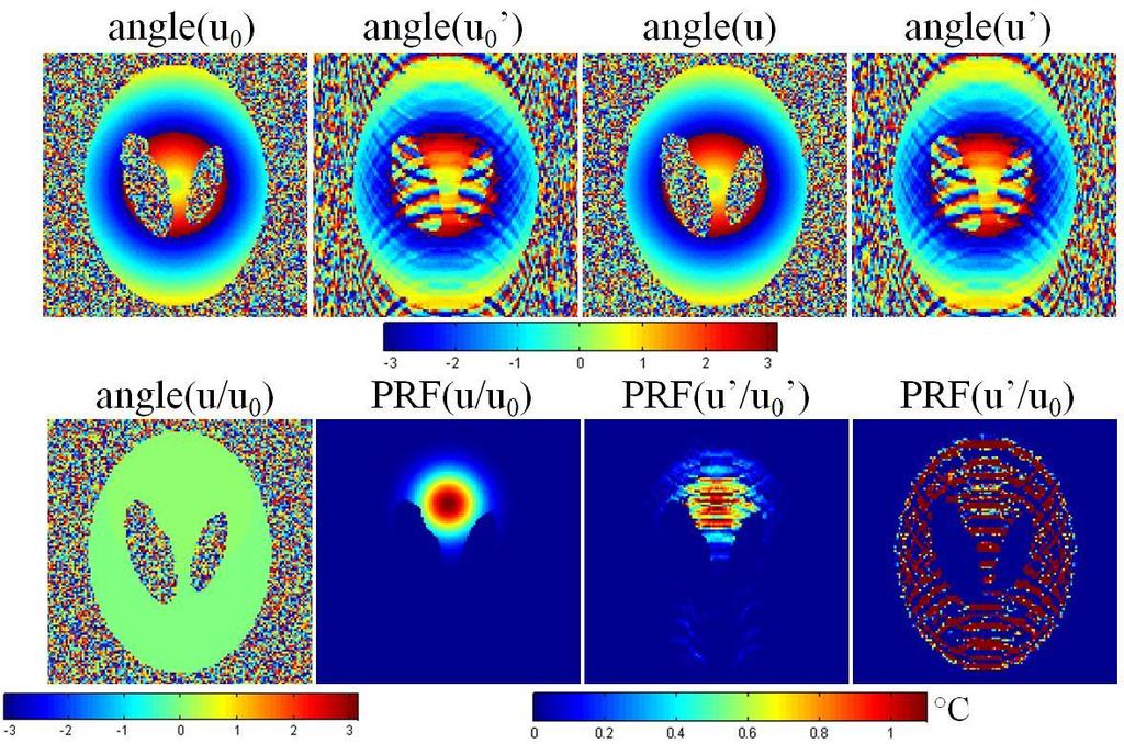
86 (a) 76

87 77 (b) Figure 5-2. Magnitude images (a), phase and masked PRF temperature change images (b) used in the simulation study. Post-heating and baseline images are denoted as u and u 0. Undersampling images are denoted with. The undersampling mask is shown in (a). The effect of proposed reconstruction method on the simulation study is demonstrated in Figure With image SNR = 1500, the proposed method reconstructed a much better PRF temperature image compared to either separated CS, or low resolution reconstructed by zero filling and FFT. Although such effectiveness decreased when image SNR dropped to 150, the method still outperformed the other two methods. Also, although phase wrapping is intentionally designed at locations of temperature changes, it is found to have no noticeable effect on the reconstruction accuracy. Figure 5-3. PRF images with different magnitude image SNRs and from various reconstruction methods, with RMSEs listed on the lower right for the heated ROI.

88 78 The results of the in vivo human forearm heating experiment are shown in Figure 5-4. The fully-sampled magnitude and phase images are first shown, followed by PRF temperature changes images, complex difference magnitude images ( u-u 0 ), and the absolute magnitude difference image in percent ratio ( u - u 0 / u 0 ). The complex difference magnitude images show close resemblance to the PRF temperature change images, proving that complex difference can be used to approximate PRF temperature change in practice. The magnitude difference image shows that changes of image magnitudes can already be found in the in vivo temperature changes (generally smaller than 10 o C) in this study.

89 79 Figure 5-4. Fully-sampled magnitude and phase images of the post-heating images, and their corresponding PRF temperature change images, complex difference magnitude images, and magnitude difference ratio images (in percent), all from the retrospective multi-slice in vivo forearm heating study. The robustness of the proposed method on a variety of temperature change patterns and sampling trajectories are demonstrated in Figure For almost all cases, the proposed method shows improved accuracy compared to separated CS and zero-filled low resolution FFT. Only one exception was found with one undersampling direction for slice 5 (Figure 5-5(e)), where the temperature change is extremely focal and close to the edge of tissue and when the

90 80 undersampling was performed in the tissue-air direction that would cause severe artifacts to the PRF temperature map. These results also showed slight changes in tissue magnitude contrast and patient motion did not detrimentally affect the reconstruction accuracy.

91 81 Figure 5-5. Reconstruction results from a retrospectively undersampled k-space dataset for in vivo human forearm heating. Results here demonstrate improved accuracy and robustness of the proposed method by using various undersampling trajectories and reconstruction methods on different imaging slices. The RMSE are shown below each error images for peak temperature error and average temperature error. These slices correspond to slices 1~5 in Figure 5-4. For the ex vivo beef heating study, the anatomical image of the beef is shown in Figure 5-6 with the location of temperature probe.

92 82 Figure 5-6. Anatomical image from the beef heating study. The arrow shows the location (red) where a fiber optic temperature probe was inserted. The reconstruction accuracy and robustness of the proposed method is demonstrated in Figure 5-7 and Figure 5-8. The reconstruction accuracy with varying degree of RF heating and PRF SNR was again demonstrated in Figure 5-7. Generally, the proposed method achieved good accuracy for all frames of the dataset, especially for the last frame (12), demonstrating its potential usage in temperature monitoring for a future time frame. It should be emphasized that such dataset was collected with system body coil that has limited image SNR, therefore the proposed method is expected to achieve better reconstruction accuracy when, for example, monitoring temperature increase of the human head using a head coil.

93 83 Figure 5-7. Reconstructed PRF images and their spatial error distributions with RMSE of different time frames from a 12-frame time series. All units are in degree Celsius. In Figure 5-8, the temporal consistency is further validated with the temperature probe reading. Temperature measurement by fully-sampled PRF images achieved very good agreement with the temperature probe reading, especially when the temperature increase is large and PRF SNR gets better. The undersampled PRF temperature readings reconstructed with the proposed method achieved excellent fidelity with the fully-sampled PRF temperature readings.

94 84 Figure 5-8. Evaluation of temporal consistency of the proposed reconstruction method by comparing with temperature probe reading and/or fully-sampled temperature change at different locations. Finally, the proposed reconstruction method is compared with the published TCR method with the beef dataset, as shown in Figure 5-9. It is shown in the result that simple modifications to the TCR method with additional L 1 or spatial TV penalty does not result in significant better reconstruction accuracy, unless the complex difference is constrained as proposed in this report.

95 85 Figure 5-9. Reconstruction accuracy demonstration of the proposed method compared to variations of previously-published method with reconstructed temperature maps listed on the left, spatial error on the right, and RMSE at the bottom. 5.6 Discussion This study proposed, validated, and demonstrated the usefulness of a modified k-t sparse reconstruction method for imaging RF heating effects with PRF thermometry by constraining the PRF temperature change through complex difference with the availability of a fully-sampled baseline image. The proposed formalism should provide improved accelerated results in situations where the expected temperature is either smooth, local or a combination of both. The effectiveness of the proposed method is proved by comparing it with classic and existed CS methods. In the demonstrated result, the proposed method not only achieved better accuracy in regions with most dramatic temperature changes, but also demonstrated improved accuracy in regions with mild temperature changes. This is especially important for SAR quantification of