EDF 7405 Advanced Quantitative Methods in Educational Research. Data are available on IQ of the child and seven potential predictors.

Transcription

1 EDF 7405 Advanced Quantitative Methods in Educational Research Data are available on IQ of the child and seven potential predictors. Four are medical variables available at the birth of the child: Birthweight (BW) the weight of the new born in grams; very large or very small weights may indicate health problems ( X ). APGAR a quick assessment of overall newborn well being. Low numbers may indicate problems ( X ). Intrapartum factors (IF) a measure of the quality of the delivery. Low numbers indicate problems occurred in the delivery ( X 3 ). Neonatal factors (NF) a measure of the health of the newborn. Low numbers may indicate health problems ( X 4 ). Three are sociological variables measured at the time of the baby s birth. Socioeconomic status a measure of the material resources available to the mother. Higher scores indicate more resources ( X 5 ). Social support a measure of the social resources available to the mother. Higher scores indicate more resources ( X 6 ). Stressful life events (SLE) a measure of the extent of stressors in the mother s life in the prior year. Higher scores indicate more stressors ( X 7 ) We want to consider the medical variables as control variables and test whether or not the sociological variables are related to IQ when the medical variables are controlled. To do this we need results for two models:

2 The full model: Y X X X X X X X The reduced model: Y X X X X In terms of the abbreviations for the variables these models are The full model: Y BW APGAR IF NF SES SS SLE The reduced model: Y BW APGAR IF NF 3 4 I present the regression results only. The residual plots for the full model should be examined before using the results for the models. Full Results See pages 8-9 of the first section for directions to conduct a regression analysis. Regression Variables Entered/Removed b Variables Entered SLE, IF, Variables Removed Method BW, SES,. Enter APGAR, SS, NF a a. All requested variables entered. b. Dependent Variable: IQ

3 3 Summary Std. Error Adjusted of the R R Square R Square Estimate.60 a a. Predictors: (Constant), SLE, IF, BW, SES, APGAR, SS, NF ANOVA b Sum of Squares df Mean Square F Sig. Regression a Residual Total a. Predictors: (Constant), SLE, IF, BW, SES, APGAR, SS, NF b. Dependent Variable: IQ Unstandardized Coefficients Coefficients a Standardi zed Coefficien ts B Std. Error Beta t Sig. (Constant) BW 5.950E APGAR IF NF 8.393E SES SS SLE a. Dependent Variable: IQ Reduced Results

4 4 See pages 8-9 of the first section for directions to conduct a regression analysis. Regression Variables Entered/Removed b Variables Entered NF, IF, Variables Removed Method APGAR, BW a. Enter a. All requested variables entered. b. Dependent Variable: IQ Summary Std. Error R R Square Adjusted R Square of the Estimate.380 a a. Predictors: (Constant), NF, IF, APGAR, BW ANOVA b Sum of Squares df Mean Square F Sig. Regression a Residual Total a. Predictors: (Constant), NF, IF, APGAR, BW b. Dependent Variable: IQ Unstandardized Coefficients Coefficients a Standardi zed Coefficien ts B Std. Error Beta t Sig. (Constant) BW 5.979E APGAR IF NF a. Dependent Variable: IQ

5 5 EDF 7405 Advanced Quantitative Methods in Educational Research SEQUENT.SAS In this handout a procedure for obtaining control-preceding variables tests is presented. Here is the SPSS Windows editor with part of the data displayed. To conduct the analysis press analyze, regression and linear

6 You get the following screen: 6

7 7 Move iq into the Dependent slot by highlighting iq and pressing the arrow to the left of the Dependent slot and bw into the Independent(s) slot by highlighting bw and pressing the arrow to the left of the independents slot. You get Now press next. You get

8 8 Notice that Block of has changed to Block of and the Independent(s) slot is empty. Move SES into the Independent(s) slot. You get Press next. You get

9 9 Notice that Block of has changed to Block 3 of 3 and the Independent(s) slot is empty. Move MAGE in the Independent(s) slot. Continue in this fashion until you have moved all independent variables into the Independent(s) and in the appropriate order. The final screen looks like this

10 0 Block 8 of 8 indicates that eight independent variables have been moved to the Independent(s) slot. Now click Statistics. The screen looks like this Unclick estimates and click R squared change. Then click continue and when the new screen opens, click OK. These results follow over several pages. Regression [DataSet] C:\7405\Spss.Programs\Third\sequent.sav Variables Entered/Removed b Variables Entered Variables Removed Method bw a. Enter ses a. Enter 3 mage a. Enter 4 apgar a. Enter 5 nf a. Enter 6 if a. Enter 7 ss a. Enter 8 sle a. Enter a. All requested variables entered. b. Dependent Variable: iq

11 In the following you will find the up to j R X in the R square column, the Type I squared semi partial correlation coefficients in the R square change column, the control-preceding-variables F statistic in the F change column and the control-precedingvariables p value in the Sig F change column. Summary Change Statistics Adjusted Std. Error of R Square R R Square R Square the Estimate Change F Change df df Sig. F Change.30 a b c d e f g h a. Predictors: (Constant), bw b. Predictors: (Constant), bw, ses c. Predictors: (Constant), bw, ses, mage d. Predictors: (Constant), bw, ses, mage, apgar e. Predictors: (Constant), bw, ses, mage, apgar, nf f. Predictors: (Constant), bw, ses, mage, apgar, nf, if g. Predictors: (Constant), bw, ses, mage, apgar, nf, if, ss h. Predictors: (Constant), bw, ses, mage, apgar, nf, if, ss, sle

12 The following results contain the F statistics for testing the omnibus multivariable hypothesis for each successive model. We do not use these results Regression Residual Total Regression Residual Total Regression Residual Total Regression Residual Total Regression Residual Total Regression Residual Total Regression Residual Total Regression Residual Total a. Predictors: (Constant), bw ANOVA i Sum of Squares df Mean Square F Sig a b c d e f g h b. Predictors: (Constant), bw, ses c. Predictors: (Constant), bw, ses, mage d. Predictors: (Constant), bw, ses, mage, apgar e. Predictors: (Constant), bw, ses, mage, apgar, nf f. Predictors: (Constant), bw, ses, mage, apgar, nf, if g. Predictors: (Constant), bw, ses, mage, apgar, nf, if, ss h. Predictors: (Constant), bw, ses, mage, apgar, nf, if, ss, sle i. Dependent Variable: iq

13 3 EDF 7405 Advanced Quantitative Methods in Educational Research Fathers are randomly assigned to either an experimental or a control group. The experimental treatment is designed to increase fathers' authoritative towards child rearing. The fathers were post tested with the Eversoll Father Role Questionnaire. In the data the control group is coded Z for the experimental group Z 0 for the control group This kind of coding is called dummy coding. The variable is denoted by a Z to emphasize that it is a categorical variable rather than a quantitative variable.

14 4 The Data Group EFRQ The model is Y Z or in terms of the abbreviations for the variables EFRQ Group The symbol is used in place of to emphasize that it is a regression coefficient for a categorical variable rather than for a quantitative variable.

15 5 The same steps that were used in simple regression analyses in the first section of the course are used again (see pages 8-9 of the first section to conduct a regression analysis). However before doing the regression analysis we must compute descriptive statistics for each group. Descriptive Statistics by Treatment Group

16 See pages 0- of the first section for directions to obtain descriptive statistics. 6

17 7 Descriptives GROUP = 0 Descriptive Statistics a EFRQ Valid N (listwise) a. GROUP = 0 Std. N Minimum Maximum Mean Deviation GROUP = Descriptive Statistics a EFRQ Valid N (listwise) a. GROUP = Std. N Minimum Maximum Mean Deviation Before conducting the regression analysis we must turn off the split-file option. To do this follow the steps used to turn it on until you get to the screen Select Analyze all cases, do not create groups and then click OK.

18 8 Regression Analysis Regression Variables Entered/Removed b Variables Entered Variables Removed Method GROUP a. Enter a. All requested variables entered. b. Dependent Variable: EFRQ Summary Std. Error R R Square Adjusted R Square of the Estimate.437 a a. Predictors: (Constant), GROUP ANOVA b Sum of Squares df Mean Square F Sig. Regression a Residual Total a. Predictors: (Constant), GROUP b. Dependent Variable: EFRQ Unstandardized Coefficients Coefficients a Standardi zed Coefficien ts B Std. Error Beta t Sig. (Constant) GROUP a. Dependent Variable: EFRQ

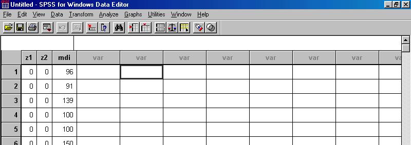
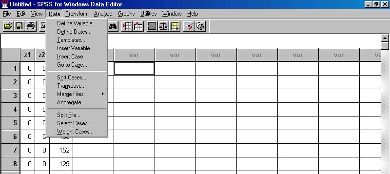
19 9 EDF 7405 Advanced Quantitative Methods in Educational Research QUAL.SAS Data are available on 5 teenage mothers and their children. The data consist of dummy variables indicating the prenatal care program in which the mother took part and mental development index (MDI) scores derived from the Bayley scales of infant development. The prenatal care was delivered by the teenage pregnancy team, private physicians, or the Shands high risk clinic. The coding of the groups is presented in the following table Prenatal Care Z Z Teenage Pregnancy Team 0 Private Physician 0 Shands High Risk Clinic 0 0 The MDI scores were obtained at age six months. The data are used to illustrate the use of regression to conduct a one-way between-subjects ANOVA. Descriptive Statistics for Each Group To get descriptive statistics on the groups, before using the Descriptive Statistics option within the Analyze option it is necessary to split the file. To review, splitting the file is done by using the Split File option within the Data option in the SPSS for Windows Data Editor.

20 0

21 Descriptives Z = 0, Z = 0 Descriptive Statistics a MDI Valid N (listwise) a. Z = 0, Z = 0 Std. N Minimum Maximum Mean Deviation Z = 0, Z = Descriptive Statistics a MDI Valid N (listwise) a. Z = 0, Z = Std. N Minimum Maximum Mean Deviation Z =, Z = 0

22 Descriptive Statistics a MDI Valid N (listwise) a. Z =, Z = 0 Std. N Minimum Maximum Mean Deviation Before running the regression analysis the file must be unsplit. Just select Analyze all cases, do not select groups in the following screen: Regression Analysis The following is the result of running the SPSS regression analysis (see pages 8-9 of the first section to conduct a regression analysis). It provided the test of the omnibus hypothesis and of the comparison of Teenage Pregnancy Team to Shands High Risk Clinic and of Private Physicians to Shands High Risk Clinic. A method for obtaining the comparison of Teenage Pregnancy Team and Private Physicians is presented after the initial regression results.

23 3 Regression Variables Entered/Removed b Variables Variables Entered Removed Method Z, Z a. Enter a. All requested variables entered. b. Dependent Variable: MDI Summary Std. Error Adjusted of the R R Square R Square Estimate.39 a a. Predictors: (Constant), Z, Z Regression Residual Total a. Predictors: (Constant), Z, Z b. Dependent Variable: MDI ANOVA b Sum of Mean Squares df Square F Sig a (Constant) Z Z a. Dependent Variable: MDI Unstandardized Coefficients Coefficients a Standardi zed Coefficien ts B Std. Error Beta t Sig

24 4 Unfortunately the SPSS regression program does not automatically produce a t statistic for comparing Teenage Pregnancy Team and Private Physicians. The t statistic can be computed by using the SPSS line code. In the following screen for the regression program press Paste: The SPSS syntax editor displays the following code: REGRESSION /MISSING LISTWISE /STATISTICS COEFF OUTS R ANOVA /CRITERIA=PIN(.05) POUT(.0) /NOORIGIN /DEPENDENT mdi /METHOD=ENTER z z Add BCOV to the statistics line: REGRESSION /MISSING LISTWISE /STATISTICS COEFF OUTS R ANOVA BCOV /CRITERIA=PIN(.05) POUT(.0) /NOORIGIN

25 5 /DEPENDENT mdi /METHOD=ENTER z z Press Run and then press All. The results will be the same as for the new full model with the exception that the following results will be added at the end. Coefficient Correlations(a) z z Correlations z z Covariances z z a Dependent Variable: mdi These results are confusingly labeled because they are not correlation coefficients and covariances for the variables. Rather they are sampling correlations and covariances. The t statistic for H0 : 0 is t S S C The results required for the denominator are Name of Statistic Sampling variance for Sampling variance for Sampling covariance for and Symbol S S C.760 Numeric value Each sampling variance is the square of a standard error, a term with which you are more familiar. The coefficients and can be found in the results labeled coefficients. These results are on page 3. Substituting in the t statistic for testing H 0 : 0

26 6 t S S C yields

27 7 EDF 7405 Advanced Quantitative Methods in Educational Research ANCORAN.SAS In the investigation of the treatment designed to increase fathers' authoritative towards child rearing, fathers were pre and post tested with the Eversoll Father Role Questionnaire. This handout illustrates how to incorporate the pretest and test for the covariate x treatment interaction. The groups are again coded The data Z for the experimental group Z 0 for the control group Group EFPOST EFPRE

28 8 for testing the interaction: The model is Y X XZ or in terms of the abbreviations of the variables EFPOST ( EFPRE) Group ( Group EFPRE). The symbol emphasizes it is a regression coefficient for the product term. We must use the TRANSFORM and COMPUTE option to add the product (GROUP EFPRE) to the data set (see pages of the first section to use the compute feature). The product is denoted by PR is the SPSS results. The following shows the resulting data See pages 6-9 of the first section for directions to produce case summaries. Summarize Case Processing Summary a Cases Included Excluded Total N Percent N Percent N Percent EFPOST % 0.0% % EFPRE % 0.0% % PR % 0.0% % a. Limited to first 00 cases.

29 9 Case Summaries a EFPOST EFPRE PR Total N a. Limited to first 00 cases.

30 30 See pages 8-9 of the first section for directions to conduct a regression analysis. Regression Variables Entered/Removed b Variables Entered PR, Variables Removed Method EFPRE, GROUP a. Enter a. All requested variables entered. b. Dependent Variable: EFPOST Summary Std. Error R R Square Adjusted R Square of the Estimate.70 a a. Predictors: (Constant), PR, EFPRE, GROUP ANOVA b Sum of Squares df Mean Square F Sig. Regression a Residual Total a. Predictors: (Constant), PR, EFPRE, GROUP b. Dependent Variable: EFPOST Unstandardized Coefficients Coefficients a Standardi zed Coefficien ts B Std. Error Beta t Sig. (Constant) GROUP EFPRE PR a. Dependent Variable: EFPOST

31 3 The evidence to this point indicates lack of support for a covariate x treatment interaction. I next show how to test the treatment effect, under the assumption that there is no covariate x treatment interaction. The groups are again coded for testing the treatment effect The model is Z for the experimental group Z 0 for the control group Y X or in terms of the abbreviations of the variables EFRQ _ POST ( EFRQ _ PRE) Group. Note that the product term has been removed. See pages 8-9 of the first section for directions to conduct a regression analysis. Regression Variables Entered/Removed b Variables Entered Variables Removed Method EFPRE, GROUP a. Enter a. All requested variables entered. b. Dependent Variable: EFPOST Summary Std. Error R R Square Adjusted R Square of the Estimate.677 a a. Predictors: (Constant), EFPRE, GROUP

32 3 Regression Residual Total ANOVA b Sum of Mean Squares df Square F Sig a a. Predictors: (Constant), EFPRE, GROUP b. Dependent Variable: EFPOST (Constant) GROUP EFPRE Unstandardized Coefficients a. Dependent Variable: EFPOST Coefficients a Standardi zed Coefficien ts B Std. Error Beta t Sig

33 33 EDF 7405 Advanced Quantitative Methods in Educational Research ANCORAN.SAS Adult children of alcoholic parents were tested using a healthy coping behaviors scale, randomly assigned to one of three treatments:. Cognitive treatment. Experiential treatment 3. Control treatment and then tested again using the healthy coping behaviors scale. Our first purpose is to test for a covariate x treatment interaction. That is, we want to determine if there is evidence for the claim that the direction and/or size of the treatment effects depends on degree of healthy coping behavior as measured by the pretest. The following are the data Treatment GROUP PRETEST POSTTEST `

34 34 for testing the interaction: The model that includes the interaction (product) terms is Y X Z Z XZ XZ or in terms of the abbreviations of the variables Post Pre Z Z Pre Z Pre Z () We must use the TRANSFORM and COMPUTE option to add the product terms to the data set (see pages of the first section to use the compute feature). These products are denoted by PR and PR in the SPSS results. The hypothesis we want to test is H : 0. 0 This is a hypothesis on a subset of the coefficients and requires us to use a full model and a reduced model. The full model is equation (). The reduced model is obtained by eliminating the coefficients in the hypothesis Post Pre Z Z. () The following are the results for the full model. See pages 8-9 of the first section for directions to conduct a regression analysis.from the model summary section we find R FM.546.

35 35 Regression Variables Entered/Removed b Variables Entered PR, PRE, Variables Removed Method Z, PR, Z a. Enter a. All requested variables entered. b. Dependent Variable: POST Summary b R R Square Adjusted R Square Std. Error of the Estimate.739 a a. Predictors: (Constant), PR, PRE, Z, PR, Z b. Dependent Variable: POST ANOVA b Sum of Squares df Mean Square F Sig. Regression a Residual Total a. Predictors: (Constant), PR, PRE, Z, PR, Z b. Dependent Variable: POST Unstandardized Coefficients Coefficients a Standardized Coefficients B Std. Error Beta t Sig. (Constant) Z Z PRE PR PR a. Dependent Variable: POST

36 36 Residuals Statistics a Minimum Maximum Mean Std. Deviation N Predicted Value Residual Std. Predicted Value Std. Residual a. Dependent Variable: POST The following are the results for the reduced model. See pages 8-9 of the first section for directions to conduct a regression analysis. From the model summary section we find R RM.504. Regression Variables Entered/Removed b Variables Entered Variables Removed Method PRE, Z, Z a. Enter a. All requested variables entered. b. Dependent Variable: POST Summary b R R Square Adjusted R Square Std. Error of the Estimate.70 a a. Predictors: (Constant), PRE, Z, Z b. Dependent Variable: POST ANOVA b Sum of Squares df Mean Square F Sig. Regression a Residual Total a. Predictors: (Constant), PRE, Z, Z b. Dependent Variable: POST

37 37 (Constant) Z Z PRE a. Dependent Variable: POST Unstandardized Coefficients Coefficients a Standardized Coefficients B Std. Error Beta t Sig Residuals Statistics a Minimum Maximum Mean Std. Deviation N Predicted Value Residual Std. Predicted Value Std. Residual a. Dependent Variable: POST To test a subset hypothesis H : 0. 0 we use the test statistic F R FM R RM nk k g R FM. In the current example we get F The critical value is F,, F.,,, and we fail to reject the null kg nk or hypothesis. Had we rejected the null hypothesis, we would have been interested in plotting the regression lines for the three groups. To do so, on the following screen

38 press Save to obtain 38

39 39 and select the unstandardized predicted values and then plot these against the pretest. See pages -3 of the first section for directions to construct a scatter plot. The following is the plot with annotations added:

40 40 Plot of Predicted Postest Score vs. Pretest 50 Score for with Product Terms Cognitive Predicted Posttest Experiential Control Pretest Since the null hypothesis was not rejected, we conclude that the following model is adequate for the data Post Pre Z Z. (3) This becomes our new full model. The hypothesis of interest is H : 0 0 Since this a hypothesis on a subset of the parameters we need a new reduced mode: Post Pre (4) We already have results for the new full model since it was out old reduced model. For this model, R FM.504. The following are the results for the new reduced model. From the model summary section we find R RM.85.

41 4 Regression Variables Entered/Removed b Variables Entered Variables Removed Method PRE a. Enter a. All requested variables entered. b. Dependent Variable: POST Summary b R R Square Adjusted R Square Std. Error of the Estimate.533 a a. Predictors: (Constant), PRE b. Dependent Variable: POST ANOVA b Sum of Squares df Mean Square F Sig. Regression a Residual Total a. Predictors: (Constant), PRE b. Dependent Variable: POST Unstandardized Coefficients Coefficients a Standardized Coefficients B Std. Error Beta t Sig. (Constant) PRE a. Dependent Variable: POST Residuals Statistics a Minimum Maximum Mean Std. Deviation N Predicted Value Residual Std. Predicted Value Std. Residual a. Dependent Variable: POST

42 4 To test the subset hypothesis H : 0 0 we use the test statistic F R FM R RM nk k g R FM. In the current example we get F The critical value is F,, F.,,, and we reject the null hypothesis. kg nk or Since we have rejected the null hypothesis H : 0 0 we want to test specific hypotheses to determine which pairs of treatments had different vertical separation between the regression lines. That is we want to test Groups Compared Cognitive vs. Control Experiential vs. Control Cognitive vs. Experiential Hypothesis H0 : 0 H0 : 0 H : 0 0 The t statistics for the first two hypotheses can be found in the coefficients section of the printout for the new full model (which was the original reduced model). These are shown in the following table:

43 43 Groups Compared Cognitive vs. Control Experiential vs. Control Cognitive vs. Experiential Hypothesis H0 : H0 : H : 0 0 t Unfortunately the SPSS regression program does not automatically produce a t statistic for a third hypothesis. The t statistic can be computed by using the SPSS line code. In the following screen for the regression program press Paste:

44 44 The SPSS syntax editor displays the following code REGRESSION /MISSING LISTWISE /STATISTICS COEFF OUTS R ANOVA /CRITERIA=PIN(.05) POUT(.0) /NOORIGIN /DEPENDENT post /METHOD=ENTER pre z z /SAVE PRED. Add BCOV to the statistics line: REGRESSION /MISSING LISTWISE /STATISTICS COEFF OUTS R ANOVA BCOV /CRITERIA=PIN(.05) POUT(.0) /NOORIGIN /DEPENDENT post /METHOD=ENTER pre z z Press Run and then press All. The results will be the same as for the new full model with the exception that the following results will be added at the end. Correlations Covariances Coefficient Correlations a Z PRE Z Z PRE Z a. Dependent Variable: POST Z PRE Z E E-0.578E E E-0. These results are confusingly labeled because they are not correlation coefficients and covariances for the variables. Rather they are sampling correlations and covariances. The t statistic for H0 : 0 is t S S C

45 45 The results required for the denominator are Name of Statistic Sampling variance for Sampling variance for Sampling covariance for and Symbol S S. C 5.49 Numeric value Each sampling variance is the square of a standard error, a term with which you are more familiar. The coefficients and can be found in the results labeled coefficients. These results are on page 4. Substituting in the t statistic for testing H 0 : 0 t S S C yields We will use the Bonferroni critical value in order to control the family wise error rate: t /,, C, nk t.05/,3,33.4

46 46 Collecting all of the results we have Groups Compared Cognitive vs. Control Experiential vs. Control Cognitive vs. Experiential Hypothesis t t /,, C, n k Decison H0 : Reject H0 : Fail to reject H : Fail to reject 0 and we conclude that there is a treatment difference between Cognitive and Control, but we do not have sufficient evidence to conclude that there is a treatment difference between Experiential and Control or between Cognitive and Experiential. The regression lines in the following plot are consistent with these results. Plot of Predicted Postest Score vs. Pretest 60 Score for without Product Terms Predicted Posttest Experiential Cognitive Control Pretest

47 47 EDF 7405 Advanced Quantitative Methods in Educational Research STEPWISE.SAS In this handout I show how to use SPSS to do stepwise regression. The data are from a textbook example. The textbook did not include a context. The data Y X X X To do stepwise regression, follow the steps to conduct a regression analysis (see pages 8-9 of the first section) until you get to the following screen.

48 48 In addition to declaring the independent and dependent variables, you must change the method to stepwise by selecting it in the drop-down menu

49 49 To make the results agree with the results in SAS I have changed some of the options. It is not necessary to change the options in order to run a stepwise regression, but SAS and SPSS will give different results if you do not. I changed the entry probability to.5 and the removal probability to.5.

50 50 Thus a coefficient that is significant at the.5 alpha level will enter the model and a coefficient that is not significant at the.5 alpha level will be removed from the model. Regression

51 5 Variables Entered/Removed a 3 4 Variables Entered X. X. X3.. X a. Dependent Variable: Y Variables Removed Method Stepwise (Criteria: Probabilit y-of-f-to-e nter <=.50, Probabilit y-of-f-to-r emove >=.5). Stepwise (Criteria: Probabilit y-of-f-to-e nter <=.50, Probabilit y-of-f-to-r emove >=.5). Stepwise (Criteria: Probabilit y-of-f-to-e nter <=.50, Probabilit y-of-f-to-r emove >=.5). Stepwise (Criteria: Probabilit y-of-f-to-e nter <=.50, Probabilit y-of-f-to-r emove >=.5).

52 5 3 4 Summary Std. Error Adjusted of the R R Square R Square Estimate.607 a b c d a. Predictors: (Constant), X b. Predictors: (Constant), X, X c. Predictors: (Constant), X, X, X3 d. Predictors: (Constant), X, X3 3 4 Regression Residual Total Regression Residual Total Regression Residual Total Regression Residual Total a. Predictors: (Constant), X b. Predictors: (Constant), X, X ANOVA e Sum of Mean Squares df Square F Sig a b c d c. Predictors: (Constant), X, X, X3 d. Predictors: (Constant), X, X3 e. Dependent Variable: Y

53 (Constant) X (Constant) X X (Constant) X X X3 (Constant) X X3 a. Dependent Variable: Y Unstandardized Coefficients Coefficients a Standardi zed Coefficien ts B Std. Error Beta t Sig X X3 X3 X Excluded Variables d Collinearit y Partial Statistics Beta In t Sig. Correlation Tolerance.56 a a b c a. Predictors in the : (Constant), X b. Predictors in the : (Constant), X, X c. Predictors in the : (Constant), X, X3 d. Dependent Variable: Y

54 54

55 55 EDF 7405 Advanced Quantitative Methods in Educational Research SUBSET.SAS SPSS does not have an all possible subsets program.

56 56 EDF 7405 Advanced Quantitative Methods in Educational Research SUBCOMP.SAS SPSS does not have an all possible subsets program.

57 57 EDF 7405 Advanced Quantitative Methods in Educational Research This shows how to use SPSS to do a multicategory logistic regression. After importing the data into the SRSS Data Editor, click Analyze, Regression, Multinomial Logistic. For my data the result is: Move MATHGRP into the dependent slot because it is the variable indicating math group membership: = Advanced; = Regular; 3 = Remedial. Move SAS into the Covariates slot. Here covariate is being used as a synonym for quantitative independent variable. The results are

58 58 Nominal Regression MATHGRP Valid Missing Total Subpopulation Case Processing Summary 3 Marginal N Percentage % % % % a a. The dependent variable has only one value observed in 5 (0.0%) subpopulations. Fitting Information Intercept Only Final Fitting Criteria Likelihood Ratio Tests - Log Likelihood Chi-Square df Sig Pseudo R-Square Cox and Snell Nagelkerke McFadden Effect Intercept SES Likelihood Ratio Tests Fitting Criteria Likelihood Ratio Tests - Log Likelihood of Reduced Chi-Square df Sig The chi-square statistic is the difference in - log-likelihoods between the final model and a reduced model. The reduced model is formed by omitting an effect from the final model. The null hypothesis is that all parameters of that effect are 0.

59 59 MATHGR a Intercep SES Intercep SES a. The reference category is: 3. Parameter Estimates B Std. Error Wald df Sig. Exp(B) Lower BoundUpper Bound % Confidence Interval fo Exp(B)

60 60

61 6 EDF 7405 Advanced Quantitative Methods in Educational Research This shows how to use SPSS to do a proportional odds logistic regression. After importing the data into the SRSS Data Editor, click Analyze, Regression, Ordinal. For my data the result is: Move MATHGRP into the dependent slot because it is the variable indicating math group membership: = Advanced; = Regular; 3 = Remedial. Move SAS into the Covariates slot. Here covariate is being used as a synonym for quantitative independent variable. The results are:

62 6 PLUM - Ordinal Regression Warnings There are 6 (0.7%) cells (i.e., dependent variable levels by combinations of predictor variable values) with zero frequencies. Case Processing Summary MATHGRP Valid Missing Total 3 Marginal N Percentage % % % % Fitting Information - Log Likelihood Chi-Square df Sig. Intercept Only Final Link function: Logit. Goodness-of-Fit Chi-Square df Sig. Pearson Deviance Link function: Logit. Pseudo R-Square Cox and Snell Nagelkerke McFadden Link function: Logit Parameter Estimates 95% Confidence Interval Estimate Std. Error Wald df Sig. Lower BoundUpper Bound Threshold [MATHGRP = [MATHGRP = Location SES Link function: Logit.