STATISTICAL ORBIT DETERMINATION

Transcription

1 STATISTICAL ORBIT DETERMINATION Satellite Tracking Example of SNC and DMC ASEN 5070 LECTURE

2 We will develop a simple state noise compensation (SNC) algorithm. This algorithm adds process noise to the acceleration equations of the system. Process-noise is added to the differential equation of motion given by Eq. (4..1), i.e., t F, t Bt t where u is white Gaussian process noise with where ij is the kronicker delta. X X u (1) T t 0, ti t j u Qti ij u u () The matrix, B, maps the process noise into the state derivatives.

3 Expanding Eq. (1) in a Taylor series about a reference trajectory, X * t, yields t t F X X X X X u X * * * t t t t B t t (3) define * t t t and At x X X F X X t t * (4) Thus the state deviation propagation equation including process noise for a linear system is given by (see Eq. (4.9.1)) t t t t t x x u (5) 3

4 We will further assume that process noise is only being added to the acceleration components of the state; hence, x y z u X 3x3 x, u u, Y x (6) 3x3 u Z y z The time update for the estimation error covariance matrix is given by Eq. (4.9.44). t k1,,, ( ) ( ), t t t t t B QB t d (7) k1 k1 k k k1 k k1 k1 t k 4

5 In this case is a constant given by Eq. (6) and t r r tk tk r tk tk 1 1 tk 1, r 1 r 1 r r r is given by, k1. (8) Each element of is a 3x3 matrix, so for simplicity define. (9) 1 t k 1, 3 4 Then 1 t k 1, (10) 5

6 One could substitute values of and 4 into Eq. (7) and carry out the integration as a quadrature. Alternatively one can approximate the values of and 4 and carry out the integration analytically. We will do the latter. From Eq. (8) we see that X t X t X t X Y Z r t Y t Y t Y t k1 k1 k1 k 1 k 1 k 1 k 1 r X Y Z Z t Z t Z t X Y Z k1 k1 k1. (11) 6

7 Because we are generally dealing with dense tracking data, the time between observations is usually 10 seconds or less. Therefore, we can assume that X () is constant over this interval X t by and approximate and k 1 X t X t (1) k1 k1 X t X k1 t k1. (13) 7

8 X t will be negligibly affected by Z. The same arguments apply to Yt and, hence Here we have assumed that for t k1 small, k 1 k 1 Z tk 1 Y and Also, tk k 1 0. (14) 0 0 tk 1 4 tk 1, r tk1 r. (15) Again the off diagonal terms are small and the diagonal terms are Aproximately=1. We assume that the velocity is constant over the interval so (, ) 1 4 t k 1 8

9 Substituting Eqs. (14) and (16) into Eq. (7) and assuming that Q is given by Define Q 0 0 X 0 Y Z k1 t t t (18) k (17) 9

10 then the process noise contribution to the estimation error covariance matrix time update at tk 1 is given by t k1 t k, ( ) ( ), t B QB t d k1 k1 3 t t X X 3 3 t t Y Y 3 t t t 0 0 t 0 0 X X t t 0 Y Y t t 3 Z z Z Z. (19) 10

11 Eq. (19) represents the contribution to the estimation error covariance matrix from uncertainty in the accelerations acting on the system. The values chosen for, and should X Y Z correspond to the magnitude of the uncertainty of the acceleration acting on the system. For example, if we were trying to compensate for atmospheric drag uncertainty this would primarily be along track. In the RTN frame one might assume that R N 0 and T corresponds to the uncertainty in the drag acceleration. A transformation to the X,Y,Z frame, which is generally ECI, would be made at each observation time so that (see Eq. ( )) Q ECI T QRTN (0) where is the transformation matrix from ECI to RTN (see Eq. (4.16.)). Note that Q ECI is not diagonal nor is it constant and Eq. (19) must be reevaluated with the proper value of Q ECI at each observation time. 11

12 The J 3 Example An ephemeris was generated for a satellite in an orbit similar to that of the Quikscat spacecraft (sun sync, 800 km, circular orbit). The propagator used in the ephemeris generation used a gravitational potential that included J and J 3 as well as atmospheric drag. Observations of range and range rate from three tracking spacecraft in Geostationary orbit were generated for a five hour data arc. Using the simulated observations containing Gaussian noise in a Kalman Filter, the position and velocity were estimated for the satellite and compared with the true values. 1

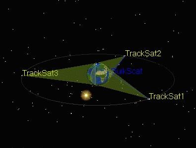
13 Tracking Configuration 13

14 The J 3 Problem Gravitational Potential Function for the J 3 Model U r 1 J R r 3sin 1 J 3 R r 3 5sin 3 3sin where sin 1 z r r x y z 14

15 J 3 Equations of Motion Taking the partials of the Gravitational Potential to get x,y,z accelerations 3 3 U x 3 Re z 5 Re z z x 1 J J x r r r r r r 3 3 U y 3 Re z 5 Re z z y 1 J J y r r r r r r 3 3 U z 3 Re z 3 Re z 35 z r z 1 J J z r r r r r 3 r z 15

16 Conventional Kalman Filter (CKF) y hxˆ y hx 16

17 Conventional Kalman Filter (CKF) RSS=4.18 m/s Velocity RSS = x 10 - m/s Position RSS = m RSS errors are based on X T (X * + ) at each stage ˆx 17

18 Extended Kalman Filter (EKF) No State Noise Added EKF implemented after 154 minutes y Hxˆ y Hx Note that pre-fit residuals for the CKF are much larger that the EKF but post-fit residuals are identical indicating that the reference trajectory for the CKF is in the linear range 18

19 Extended Kalman Filter (EKF) Velocity RSS = 4.33 x 10 - m/s Position RSS = m RSS position and velocity errors for CKF and EKF are nearly identical 19

20 Band Diagonal State Noise Matrix 3 t t X X 3 3 t t Y Y 3 t t T Q 3 t 0 0 t 0 0 X X t t 0 Y Y t t 3 Z Z Z Z See web page handouts or previous slides for derivation 0

21 Conventional Kalman Filter with SNC Band Diagonal State Noise Matrix results for optimum value: = y Hxˆ y hx y hx 1

22 Conventional Kalman Filter with SNC Band Diagonal State Noise Matrix results for optimum value: = Velocity RSS = 1.6 x 10 - m/s Position RSS = 8.43 m

23 Conventional Kalman Filter with SNC Band Diagonal State Noise Matrix results for optimum value: = Kalman gain is so large that data is fit almost perfectly well below noise levels of 1cm and 1mm/s This is what happens if an input error inject a huge amount of process noise i.e. = instead of

24 Conventional Kalman Filter with input error Band Diagonal State Noise Matrix results for optimum value: = standard deviations of estimation error covariance are red lines Velocity RSS = 1. x 10 - m/s Position RSS = m Small residuals do not a good orbit Make RSS errors are larger than Previous results 4

25 Extended Kalman Filter with State Noise (SNC) Band Diagonal State Noise Matrix 3 t t X X 3 3 t t Y Y 3 t t T Q 3 t 0 0 t 0 0 X X t t 0 Y Y t t 3 Z Z Z Z 5

26 Extended Kalman Filter with State Noise (SNC) Band Diagonal State Noise Matrix Looked for optimum values of by analyzing residuals and errors Optimum value to minimize position errors: =

27 Extended Kalman Filter with State Noise (SNC) Band Diagonal State Noise Matrix results for optimum value: = y Hxˆ y Hx y ( recall that x 0) 7

28 Extended Kalman Filter with State Noise (SNC) Band Diagonal State Noise Matrix results for optimum value: = Velocity RSS = x 10 - m/s Position RSS = 8.50 m Position RSS = 8.50 m The CKF and EKF results are Nearly identical indicating that Initial conditions are in the linear range 8

29 Extended Kalman Filter with Fading Adds a fading term to the time update this downweights earlier data by Keeping the Kalman gain elevated P i s(t i,t i1 )P i1 T (t i,t i1 ) where t s e >1 t = time between measurements = 0 seconds = age-weighting time constant 9

30 Extended Kalman Filter with Fading Looked for optimum value of s to minimize the residuals and errors Optimum value of s ~ This corresponds to a of 10 minutes 30

31 Extended Kalman Filter with Fading Optimum values of s to minimize position and velocity errors : s = y Hxˆ x y 31

32 Extended Kalman Filter with Fading Optimum values of s to minimize position and velocity errors : s = Velocity RSS = x 10 - m/s Position RSS = m Position RSS=8.688 m 3

33 Kalman Filter Results Comparison Conventional Kalman Extended Kalman Filter State Noise Matrix State Noise Matri Fading N/A N/A N/A Ra nge Residual (m) Ra nge Rate Residua l (m) E E E-03 X Position Erro r (m) Y Position Erro r (m) Z Position Erro r (m) Position RSS (m) X Velocity Error (m/s) 1.41E E E-0 5.7E E-03 Y Velocity Error (m/s) 3.0E E E E E-03 Z Velocity Error (m/s).66e-0 1.1E-0.58E E-0 1.1E-0 Velocity RSS (m/s) 4.394E-0 1.6E E E E-0 Conclusions: The CKF and EKF produce comparable results indicating that the reference orbit for the CKF is in the linear range for this example. Fading produces comparable results to SNC 33

34 Dynamic Model Compensation (DMC) DMC accounts for unmodeled or inaccurately modeled accelerations acting on the spacecraft - J 3 in this problem. The state vector was augmented to the following: X x, y, z, x, y, z, x, y, z where x, y, and z are the accelerations A Gauss-Markov process is used to account for these accelerations: ( t) ( t) u( t) where u(t) is white Gaussian noise with E(u) 0 Eu(t)u() (t ) and 1 Where is a time constant 34

35 Dynamic Model Compensation and were optimized to give the lowest position and velocity errors: 10 orbital period =

36 Dynamic Model Compensation Optimized Results Velocity RSS = 1.49 x 10 - m/s Position RSS = m 36

37 Dynamic Model Compensation Optimized Results Actual vs estimated accelerations Errors in acceleration estimates in x,y, And z directions Note: the DMC did a poor job of recovering accelerations. More work is needed on optimizing and.we should do a better job of recovering accelerations and the state while reducing tracking residuals. 37

38 Filter Comparisons Conventional Kalman Extended Kalman Filter DMC State Noise Matrix State Noise Matri Fading N/A N/A N/A Ra nge Residual (m) Ra nge Rate Residual (m) E E E E-03 X Position Error (m) Y Position Error (m) Z Position Error (m) Position RSS (m) X Velocity Error (m/s) 1.41E E E-0 5.7E E E-03 Y Velocity Error (m/s) 3.0E E E E E E-03 Z Velocity Error (m/s).66e-0 1.1E-0.58E E-0 1.1E E-0 Velocity RSS (m/s) 4.394E-0 1.6E E E E E-0 All filters achieved comparable results; however we should do better with the DMC 38

39 Added deviations to the initial conditions so that they are outside linear range to show Convergence for EKF with SNC Divergence for CKF with SNC Original Initial Conditions [ , , , , , ] m and m/s Deviation [8, 5, 5, 8, 5, 5] m and m/s Perturbed Initial Conditions [ , , , , , ] m and m/s 39

40 Conventional Kalman Filter Band Diagonal State Noise Matrix results for optimum value: = Deviated Initial Conditions y hxˆ y Hx y hx 40

41 Conventional Kalman Filter Band Diagonal State Noise Matrix results for optimum value: = Deviated Initial Conditions Velocity RSS =.88 m/s Position RSS = m 41

42 Extended Kalman Filter Band Diagonal State Noise Matrix results for optimum value: = Deviated Initial Conditions y Hxˆ y Hx y 4

43 Extended Kalman Filter Band Diagonal State Noise Matrix results for optimum value: = Deviated Initial Conditions Velocity RSS =.53 x 10 - m/s Position RSS = m 43

44 Filter Comparisons CKF EKF Initial Co nditions Linear R ange Nonlinear R ange Linear R ange Nonlinear R ange Ra nge Residual (m) Ra nge Rate Residual (m) 6.64E E E E-0 X Position Erro r (m) Y Position Erro r (m) Z Position Erro r (m) Position RSS (m) X Velocity Error (m/s) 6.19E E E E-03 Y Velocity Error (m/s) 8.89E E E-0 Z Velocity Error (m/s) 1.1E E E-0 3D Velocity RSS (m/s) 1.6E E-0.58E-0 While the CKF does not diverge, its solution is significantly In error 44

45 Added deviations to the initial conditions to show Convergence for EKF with SNC Divergence for the Batch Processor Original Initial Conditions [ , , , , , ] m, m/s Deviation [1000, 1000, 1000, 500, 500, 500] m,m/s Perturbed Initial Conditions [ , , , , , ] m, m/s 45

46 Batch Processor Pass 1 Range RMS = km Range rate RMS = km/s Pass 3 Range RMS = km Range rate RMS = km/s Note that the batch processor is not converging and successive Iterations show divergence 46

47 Extended Kalman Filter Band Diagonal State Noise Matrix results for various values of Deviated Initial Conditions Trajectory updated after 30 minutes Note: Values of from 10-5 to 10-0 were tested. However, the residuals and errors were orders of magnitude higher for value of between 10-5 to Therefore, those values are not shown on the plots. Note that the optimal value for is the same as for small initial condition errors. 47

48 Extended Kalman Filter Band Diagonal State Noise Matrix results for = Deviated Initial Conditions Trajectory updated after 30 minutes y Hxˆ y y 48

49 Extended Kalman Filter Band Diagonal State Noise Matrix results for = Deviated Initial Conditions Position Errors after 50 minutes Position Errors Position RSS = m 49

50 Extended Kalman Filter Band Diagonal State Noise Matrix results for = Deviated Initial Conditions Velocity Errors after 50 minutes Velocity Errors Velocity RSS = 1.58 x 10 - m/s Note that position and velocity RSS are comparable to those on slide 40. If IC errors are large it may be Colorado Center Advantageous for Astrodynamics to use the Research EKF to The University Obtain of Colorado ICs for the batch 50

51 Transformation of State and Covariance Matrix to Alternate Frames Sometimes it is desirable to transform the state vector and the estimation error covariance into alternate coordinate systems. It may be of interest to view these quantities in a radial, transverse, and normal (RTN) system. The general transformation between any two coordinate frames (say prime to unprimed) for a position vector is given by r r a, ( ) where is an orthogonal transformation matrix. r is the vector in the unprimed frame, and a is the vector offset of the origin of the two systems. 51

52 Transformation of State and Covariance Matrix to Alternate Frames The velocity transforms according to r rr ( ) Generally will be zero unless we are transforming from a rotating to a nonrotating frame or vice versa; for example, ECEF to ECI. It can be shown that r r, where is the angular velocity of the rotating frame. The transformation we want is ECI to RTN. We assume that the RTN frame is fixed to the osculating orbit at each point in time; hence 0 and r 0 r 0 v v RTN ECI. ( ) 5

53 Transformation of State and Covariance Matrix to Alternate Frames The covariance of the estimation error is transformed as follows: xˆ x xˆ x, RTN ECI where 0 0 rˆ r 0 0 and ˆ ˆ x x v v, ( ) 0 0 I ˆ and r, v, and represent the true values of the position, velocity, and all other quantities in the state vector, respectively. It is assumed that none of the elements of are affected by the coordinate transformation. 53

54 Transformation of State and Covariance Matrix to Alternate Frames The desired covariance is given by P RTN xˆ xxˆ x E x xx x RTN T T E ˆ ˆ. T ECI ( ) The elements of for the ECI to RTN transformation are given by R T N r * u i j k r * r* v* u i j k, r* v* X Y Z u u u i j k N R X Y Z X Y Z (4.16.0) where ur, ut, u N are unit vectors in the RTN frame, i, j, and k are unit vectors in the ECI frame, and r* and v* are the position and velocity vectors of the reference orbit. 54

55 Transformation of State and Covariance Matrix to Alternate Frames Equation (4.16.0) may be written ur X Y Z i u j. (4.16.1) T X Y Z u N X Y Z k Hence, the transformation matrix relating the RTN and ECI frame is X Y Z X Y Z. (4.16.) X Y Z The transformation relating the covariance matrix in two different frames is P P. B B A A B A T 55

56 Transformation of State and Covariance Matrix to Alternate Frames Assume we wish to transform Φ(t i, t j ) from the A frame to the B frame r t i x( ti ) v ti Let Recall that and x( ti ) ( ti, t j ) x( t j ) A A A A B x( t ) x( t ) i B T 0 T 0 A B x( t ) A B i A i A 56

57 Transformation of State and Covariance Matrix to Alternate Frames But Hence, x( ti ) B ti, t j ( t j ) B x A A B B ti, t j A x( t j ) x( ti ) ( ti, t j ) x( t j ) B B B t, t A t, t B i j B B i j A A A A A B where B A A B T 57