EC 624 Digital Image Processing ( ) Class I Introduction. Instructor: PK. Bora

Transcription

1 EC 624 Digital Image Processing ( ) Class I Introduction Instructor: PK. Bora

2 Digital Image Processing Digital Image Processing means processing of digital images on digital hardware usually a computer

3 What is an analog image? Electrical Signal, for example, the output of a video camera, that gives the electric voltage at locations in an image

4 What is a digital Image 2D array of numbers representing the sampled version of an image The image defined over a grid, each grid location being called a pixel. Represented by a finite grid and each intensity data is represented a finite number of bits. A binary image is represented by one bit gray-level image is represented by 8 bits. Pixel and Intensities

5 Mathematically We can think of an image as a function, f, from R 2 to R: f( x, y ) gives the intensity at position ( x, y ) Realistically, we expect the image only to be defined over a rectangle, with a finite range: f: : [a,[ b]x[c, d] [0, 1]

6 What is a Colour Image? Three components: R,G, B each usually represented by 8 bits We call 24-bit video These three primary are mixed in different proportions to get different colours For different processing applications other formats (YIQ,YCbCr,, HIS etc) are used A color image is just a three component function. We can write this as a vector-valued function: rxy (, ) f ( xy, ) = gxy (, ) bxy (, )

7 Types of Digital Image Digital images include Digital photos Image sequences used for video broadcasting and playback Multi-sensor data like satellite images in the visible, infrared and microwave bands Medical images like ultra-sound, Gamma-ray images, X-ray images and radio-band images like MRI etc Astronomical images Electron-microscope images used to study material structure

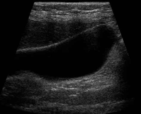
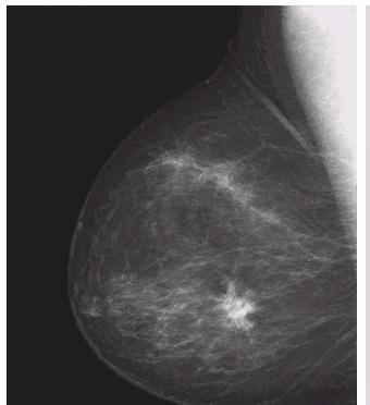
8 Photgraphic Examples Ultrasound Mammogram

9 Image processing Digital Image processing deals with manipulation and analysis of the digital image by a digital hardware, usually a computer. Emphasizing certain pictorial information for better clarity (human interpretation) Automatic machine processing of the scene data. Compressing the image data for efficient utilization of storage space and transmission bandwidth

10 Image Processing An image processing operation typically defines a new image g in terms of an existing image f. We can also transform O the domain of f:

11 Image Processing image filtering: change range of image f h f x g(x) ) = h(f(x)) x image warping: change domain of image f h f x g(x) ) = f(h(x)) x

12 Example Image Restoration Degraded Image Processing Restored Image

13 Image Processing steps Acquisition, Sampling/ Quantization/ Compression Image enhancement and restoration Feature Extraction Image Segmentation Object Recognition Image Interpretation

14 Image Acquisition An analog image is obtained by scanning the sensor output. Some of the modern scanning device such as a CCD camera contains an array of photo- detectors, a set of electronic switches and control circuitry all in a single chip

15 Image Acquisition Image Sensor Sample and Hold Analog to to Digital Takes a measurement and holds it for conversion to digital. Converts a measurement to digital Digital Image

16 Sampling/ Quantization/ Compression A digital image is obtained by sampling and quantizing an analog image. The analog image signal is sampled at rate determined by the application concerned Still image 512X512, 256X256 Video: 720X480, 360X240, 1024x 768 (HDTV) The intensity is quantized into a fixed number of levels determined human perceptual limitation 8 bits is sufficient for all but the best applications 10 bits Television production, printing bits Medical imagery

17 Sampling/ Quantization/ Compression (Contd.) Raw video is very bulky Example:The transmission of high- definition uncompressed digital video at 1024x 768, 24 bit/pixel, 25 frames requires 472 Mbps We have to compress the raw data to store and transmit

18 Image Enhancement Improves the qualities of an image by enhancing the contrast sharpening the edges removing noise, etc. As an example, let us explain the image filtering operation to remove noise.

19 Example: Image Filtering Original Image Filtered Image

20 Histogram Equalization Enhance the contrast of images by transforming the values in an intensity image to its normalized histogram the histogram of the output image is uniformly distributed. Contrast is better

21 Feature Extraction Extracting Features like edges Very important to detect the boundaries of the object Done through digital differentiation operation

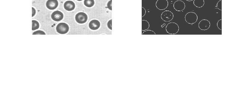
22 Example: Edge Detection Original Saturn Image Edge Image

23 Segmentation Partitioning of an image into connected homogenous regions. Homogeneity may be defined in terms of: Gray value Colour Texture Shape Motion

24 Segmented Image

25 Object Recognition An object recognition system finds objects in the real world from an image of the world, using object models which are known a priori labelling problem based on models of known objects

26 Object Recognition (Contd.) Object or model representation Feature extraction Feature-model matching Hypotheses formation Object verification

27 Image Understanding Inferring about the scene on the basis of the recognized objects Supervision is required Normally considered as part of artificial intelligence

28 Books 1. R. C. Gonzalez and R. E. Woods, Digital Image Processing,, Pearson Education, 2001 (Main Text) 2. A. K. Jain, Fundamentals of Digital Image processing,, Pearson Education, R. C. Gonzalez, R. E. Woods and S. L. Eddins, Digital Image Processing using MATLAB, Pearson Education, (Lab Ref)

29 Evaluation Scheme End Sem 50 Mid Sem 25 Quiz 5 Matlab Assignment 10 Mini Project 10 Total 100

30 1. MINI PROJECT Matlab Implementation and preparing Report and Demonstration of any advanced topic like: Video compression Video mosaicing Video-based tracking Medical Image Compression Video Watermarking Medical Image Segmentation Image and Video Restoration Biometric recognition

31 2D Discrete Time (Space) Fourier Transform Recall DTFT of a 1D sequence, Given X ω e ω ( ) = x[ n] n=- [ ] { xn, n=... } j n is and Note that 1 2π [ ] X( ω) xn = π π ( + 2 ) = X( ) X ω π ω e jωn dω ( ) exists if and only if X ω x[ n] is absolutely summable, i.e., n= [ ] xn <

32 Relationship between CTFT and DTFT Consider a discrete sequence { xn [ ], n=... } obtained by sampling an analog signal xa ( t) at a uniform sampling rate 1 F, where T is s = the sampling period. T We can represent the sampling process by means of the Dirac delta function with the relation [ ] = ( ), n=0, ± 1... xn x nt Now the sampled signal can be represented in continuous domain as, () = x () δ ( ) x t t t nt s = x a n=- n=- a a ( nt ) δ ( t nt ) Thus, the analog and discrete frequencies are related as w= ΩT.

33 2D DSFT Consider the signal two-dimensional space. { f[ m, n], m=,...,, n=,..., } defined over the Also assume m= n= f[ m, n] <. Then the two-dimensional discrete-space Fourier transform (2D DSFT) and its inverse are defined by the following relations: and F( u, v) = n= m= f [ m, n] e j( um+ vn) 1 + jum ( + vn) f [ mn, ] = Fuve (, ) du dv 2 4π

34 F( uv, ) Note that is doubly periodic in u and v. Following properties of F( uv, ) are easily verified: Linearity Separability Shifting theorem: Convolution theorem: If fmn [, ] 2 D DSFT ( vn) 2 D DSFT 0 0 [, ] (, ), 0 0 Fuv (, ), then jum+ f m m n n e F u v If f [ m, n] F( u, v) and f [ m, n] F ( u, v), then 2 D DSFT 2 D DSFT f [ m, n])* f [ m, n] F( u, v) F ( u, v) 2 D DSFT Eigen function Modulation Correlation Inner product Parseval s theorem

35 2D DFT Motivation Consider the 1D DTFT which is uniquely defined for each ω. [0, 2 π ]. X( ω) = x[ ne ] X ( ω) n= Numerical evaluation of involves very large (infinite) data and is to be done for each ω. An easier way is the Discrete Fourier transform (DFT) which is obtained by sampling X ( ω) at a regular interval. 1 N jwn 1 Sampling periodically in the frequency domain at a rate means that the data sequence will be periodic with a period N N. The relation between the Fourier transform of an analog signal x a (t) and the DFT of the sampled version is illustrated in the Figure below.

36 2D DFT The 2D DFT of a 2D sequence is defined as N-1 M-1 2π 2π j mk1+ nk2 M N 1 2 = 1 = 2 n= 0 m= 0 [ ] [ ] F k, k f m, n e, k 0,1,..., M 1, k =0,1,...,N-1 and the inverse 2D DFT is given by k and k 1 2 k =0 k =0 2 1 j 2π mk 2π 1 nk + 2 M N N-1 M-1 1 f [ m, n] = F[ k 1, k2] e, m= 0,1,..., M 1, n=0,1,...,n-1 MN 2D DFT is periodic in both Thus Fk [, k] = Fk [ + Mk, + N]

37 Properties of 2D DFT Shifting property 2 D DFT If f[ m, n] F[ k1, k2], then 2 2 j m0k1 n0k2 2 D DFT + M N f [ m m, n n ] e F[ k, k ] π π Separability propery Since 2π 2π j mk nk 2π 2π + j mk j nk M N M N = e e e

38 Thus the 2D DFT can be computed from a 1D FFT routine Properties of 2D DFT Separability propery Since 2π 2π j mk nk 2π 2π + j mk j nk M N M N = e e e We can write N -1 M -1 2 π 2 π j m k + n k M N [, ] = [, ] F k k f m n e n = 0 m = 0 N -1 M -1 2 π j m k = [, ] n = 0 m = 0 = N -1 n = 0 F [ k, n ] e [ ] M f m n e e 2 π j n k N w here F [ k, n ] = f m, n e M m = π j m k M 1 2 π j N nk 2

39 2D Fourier Transform Frequency domain representation of 2D signal :: x, y. ( ) Consider a two-dimensional signal The signal f ( x, y) and its two-dimensional Fourier transform are related by :: f x, y F( u, v) u and v represent the spatial frequency in radian/length. F(u,v) represents the component of f(x,y) with frequencies u and v. A sufficient condition for the existence of F(u,v) is that f(x,y) is absolutely integrable. f ( ) 2DFT j( xu+ yv) F u v f x y e dx dy (, ) (, ) = 1 j( xu + yv) f ( x, y) = F ( u, v) e du dv 2 4π f( x, y) dxdy < F ( uv, )

40 2D Fourier Transform u and v represent the spatial frequency in horizontal and vertical directions inradian/length. F(u,v) represents the component of f(x,y) with frequencies u and v. Illustration of 2D Fourier transform

41 2D Fourier Transform A sufficient condition for the existence of F(u,v) is that f(x,y) is absolutely integrable. f( x, y) dxdy <

42 Properties of 2D Fourier Transform 1. The 2D Fourier transform is in general a complex function of the real variables uand v. As such, it can be expressed in terms of the magnitude Fuv (, ) and the phase F( uv, ). 2. Linearity Property: f ( x, y) F( u, v) 2D FT 1 1 f ( x, y) F ( u, v) 2D FT 2 2 a f ( x, y) + bf ( x, y) af( uv, ) + bf( uv, ) 2D FT Shifting Property: f ( x x o, y y o 2D FT ) e j( xo u+ y o v) F( u, v) Phase information changes, no change in amplitude. 4. Modulation Property: f ( x, y) e + j( u o x+ v o y) F( u u o, v v o )

43 5. Complex exponentials are the eigen functions of linear shift invariant systems. The Fourier bases are the Eigen functions of linear systems For an imaging system, h(x, y) is called the point spread function and H (u, v) is called the optical transfer function

44 6. Separability property: jux jvy F( u, v) = f ( x, y) e dx. e dy where = f ( x, y) = f1( x) f2( y) 1 F ( u, v) e Particularly if then jvy dy F ( u, v) is 1-D Fourier Transform F( uv, ) = F( uf ) ( v) Suppose x y f ( x, y) = rect. rect a a, then F uv, = asincau asincav ( ) ( ) 2 = a sincau sincav

45 7. 2D Convolution: If g( x, y) = f( x, y)* hxy (, ) Guv (, ) = FuvHuv (, ) (, ) Similarly if g( x, y) = f( x, y) hxy (, ) 1 Guv (, ) = Fuv (, )* Huv (, ) 2 4π Thus the convolution of two functions is equivalent to product of the corresponding Fourier transforms.

46 8. Preservation of inner product: Recall that the inner product of two functions is defined by f( x, y), h( x, y) f( x, y) h( x, y) dx dy = The inner product is preserved through Fourier transform. Thus, 1 f( x, y), h( x, y) = F( u, v), H( u, v) 2 4π where Fuv (, ), Huv (, ) FuvHuv (, ) (, ) du dv = f ( x, y) and h( x,y) Particularly, 1 f( x, y), f( x, y) = F( u, v), F( u, v) 2 4π f ( x, y) dx dy = F( u, v) du dv 2 4π Hence Norm is preserved through 2D Fourier transform.

47 2D Discrete Time (Space) Fourier Transform Recall DTFT of a 1D sequence, Given X ω e ω ( ) = x[ n] n=- [ ] { xn, n=... } j n is and Note that 1 2π [ ] X( ω) xn = π π ( + 2 ) = X( ) X ω π ω e jωn dω ( ) exists if and only if X ω x[ n] is absolutely summable, i.e., n= [ ] xn <

48 Relationship between CTFT and DTFT Consider a discrete sequence { xn [ ], n=... } obtained by sampling an analog signal xa ( t) at a uniform sampling rate 1 F, where T is s = the sampling period. T We can represent the sampling process by means of the Dirac delta function with the relation [ ] = ( ), n=0, ± 1... xn x nt Now the sampled signal can be represented in continuous domain as, () = x () δ ( ) x t t t nt s = x a n=- n=- a a ( nt ) δ ( t nt ) Thus, the analog and discrete frequencies are related as w= ΩT.

49 2D DSFT Consider the signal two-dimensional space. { f[ m, n], m=,...,, n=,..., } defined over the Also assume m= n= f[ m, n] <. Then the two-dimensional discrete-space Fourier transform (2D DSFT) and its inverse are defined by the following relations: and F( u, v) = n= m= f [ m, n] e j( um+ vn) 1 + jum ( + vn) f [ mn, ] = Fuve (, ) du dv 2 4π

50 F( uv, ) Note that is doubly periodic in u and v. Following properties of F( uv, ) are easily verified: Linearity Separability Shifting theorem: Convolution theorem: If fmn [, ] 2 D DSFT ( vn) 2 D DSFT 0 0 [, ] (, ), 0 0 Fuv (, ), then jum+ f m m n n e F u v If f [ m, n] F( u, v) and f [ m, n] F ( u, v), then 2 D DSFT 2 D DSFT f [ m, n])* f [ m, n] F( u, v) F ( u, v) 2 D DSFT Eigen function Modulation Correlation Inner product Parseval s theorem

51 Colour Image Processing Colour plays an important role in image processing Colour image processing can be divided into two major areas Full-colour processing: Colour sensors such as colour cameras and colour scanners are used to capture coloured image. Processing involves enhancement and other image processing tasks Pseudo-colour processing : Assigning a colour to a particular monochrome intensity range of intensities to enhance visual discrimination.

52 Colour Fundamentals Visible spectrum: approx. 400 ~ 700 nm The frequency or mix of frequencies of the light determines the colour Visible colours: VIBGYOR with UV and IR at the two extremes (excluding)

53 HVS review Cones are the sensors in the eye responsible for colour vision Humans perceive colour using three types of cones Primary colours: RGB because the cones of our eyes can basically absorb these three colours. The sensation of a certain colour is produced due to the mixed response of these three types of cones in a certain proportion Experiments show that 6-7 million cones in the human eye can be divided into red, green and blue vision. 65% cones are sensitive to red vision, 33% are for green and only 2% are for blue vision (blue cones are the most sensitive)

54 Experimental curves for colour Sensitivity Absorption of light by red, green and blue cones in the human eye as a function of wavelength

55 Colour representations: Primary colours According to the CIE (Commission Internationale de l Eclairage, The International Commission on Illumination) the wavelength of each primary colour is set as follows: blue=435.8nm, green=546.1nm, and red=700nm. However this standard is just an approximate; it has been found experimentally that no single colour may be called red, green, or blue There is no pure red, green or blue colour. The primary colours can be added in certain proportions to produce different colours of light.

56 Natural and Artificial Colour The colour produced by mixing RGB is not a natural colour. A natural colour will have a single wavelength, say λ. On the other hand, the same colour is artificially produced by combining weighted R, G and B each having different wavelength. The idea is that these three colours together will produce the same amount of response as that would have been produced by wavelength λ alone (proportion of RGB is taken accordingly), thereby giving the sensation of the colour with wavelength λ to some extent.

57 Colour representations: Secondary colours Mixing two primary colours in equal proportion produces a secondary colour of light: magenta (R+B), cyan (G+B) and yellow (R+G). Mixing RGB in equal proportion produces white light. The second figure shows primary/secondary colours of pigments.

58 Colour representations: Secondary colours There is a difference between the primary colours of light and primary colours of pigments. Primary colour of a pigment is defined as one that subtracts or absorbs a primary colour of light and reflects or transmits the other two. Hence, the primary colours of pigments are magenta, cyan, and yellow. Corresponding secondary colours are red, green, and blue.

59 Brightness, Hue, and Saturation Brightness perceived (subjective brightness) is a logarithmic function of light intensity. In other words it embodies the chromatic notion of intensity. Hue is an attribute associated with the dominant wavelength in a mixture of light waves. It represents the dominant colour as perceived by an observer. Thus, when we call an object red, orange, or yellow, we are specifying its hue. Saturation refers to the relative purity or the amount of white light mixed with hue. The pure spectrum colours are fully saturated. colour such as pink (red and white) is less saturated. The degree of saturation is inversely proportional to the amount of white light added.

60 Brightness, Hue, and Saturation (contd..) Red, Green, Blue, Yellow, Orange, etc. are different hues. Red and Pink have the same hue, but different saturation. A faint red and a piercing intense red have different brightness. Hue and saturation taken together are called chromaticity. So, brightness + chromaticity defines any colour.

61 XYZ Colour System CIE (Commision Internationale de L Eclairage), Spectral RGB primaries (scaled, such that X=Y=Z matches spectrally flat white). The entire colour gamut can be produced by the three primaries used in CIE 3-colour system. A particular colour (of wavelength λ) be represented by three components X, Y, and Z. These are called tri-stimulus values. X Rλ Y = G λ Z Bλ λ denotes corresponding spectral component

62 Colour composition using XYZ XYZ Colour System A colour is then specified by its tri-chromatic coefficients, defined as x= X/(X+Y+Z) y= Y/(X+Y+Z) z = Z/(X+Y+Z) so that x + y +z=1 For any wavelength of light in the visible spectrum, these values can be obtained directly from curves or tables compiled from experimental results.

63 Chromaticity Diagram Shows colour composition as a function of x and y (only two of x, y and z are independent z = 1 (x + y) and so not independent of them) The triangle in the diagram below shows the colour gamut for a typical RGB system plotted as the XYZ system. 1 y The axes extend from 0 to 1. The origin corresponds to BLUE. The extreme points on the axes correspond to RED and GREEN.The point corresponding to x= y= 1/3 (marked by the white spot) corresponds to WHITE. 0 1 x

64 Actual Chromaticity Diagram The positions of various spectrum colours from violet (380nm) to red (700 nm) are indicated around the boundary (100% saturation). These are pure colours. Any inside point represents mixture of spectrum colours. A straight line joining a spectrum colour point to the equal energy point shows all the different shades of the spectrum colour.

65 Any color in the interior of the horse shoe" can be achieved through the linear combination of two pure spectral colors A straight line joining any two points shows all the different colours that may be produced by mixing the two colours corresponding to the two points The straight line connecting red and blue is referred to as the line of purples

66 RGB primaries form a triangular color gamut. The white colour falls in the center of the diagram W

67 Colour vision model: RGB colour Model Colour models are normally invented for practical reasons, and so a wide variety exist. The RGB colour space (model) is a linear colour space that formally uses single wavelength primaries. Informally, RGB uses whatever phosphors a monitor has as primaries Available colours are usually represented as a unit cube usually called the RGB cube whose edges represent the R, G, and B weights. Schematic of the RGB colour cube RGB 24-bit colour cube

68 CMY and CMYK colour models Cyan, Magenta, Yellow Primary pigment colour Subtractive color space Related to RGB by C 1 M = 1 Y 1 Should produce black C 1 R M = 1 G Y 1 B Practical printing devices additional black pigment is needed. This gives the CMYK colour space

69 Decoupling the colour components from intensity Decoupling the intensity from colour components has several advantages: Human eyes are more sensitive to the intensity than to the hue We can distribute the bits for encoding in a more effective way. We can drop the colour part altogether if we want gray-scale images. In this way, black-and-white TVs can pick up the same signal as color ones. We can do image processing on the intensity and color parts separately. Example: Histogram equalization on the intensity part to contrast enhance the image while leaving the relative colors the same

70 HSI Colour system Hue is the colour corresponding to the dominant wavelength measured in angle with reference to the red axis Saturation measures the purity of the colour. In this sense impurity means how much white is present. Saturation is 1 for a pure colour and less than 1 for an impure colour. Intensity is the chromatic equivalent of brightness also means the grey level component. S I H I

71 HSI Colour Model HSI model can be obtained from the RGB model. The diagonal of the joining Black and White in the RGB cube is the intensity axis

72 HSI Model

73 HSI Colour Model HSI colour model based on a triangle and a circle are shown The circle and the triangle are perpendicular to the intensity axis.

74 [ ] [ ] ( ) [ ] ) ( 3 1 ),, min( 3 1 ) )( ( ) ( ) ( ) ( 2 1 cos if 360 if B G R I B G R B G R S B G B R G R B R G R G B G B H o + + = + + = + + = > = θ θ θ Conversion from RGB space to HSI The following formulae show how to convert from RGB space to HSI:

75 Conversion from RGB space to HSI To convert from HSI to RGB, the process depends on which colour sector H lies in. For the RG sector: For the GB sector: For the BR sector: o 0 H 120 o 120 o o H 240 o 240 o H 360 H = H 240 G= I(1 S) B= I 1 + R= 3I ScosH cos60 ( H) ( G+ B) B= I(1 S) R= I 1 + G= 3I H= H 120 R= I(1 S) ScosH cos60 ( H) ( R+ B) ScosH G= I 1+ cos 60 B= 3I R+ G ( H) ( )

76 YIQ model YIQ colour model is the NTSC standard for analog video transmission Y stands for intensity I is th e in phase component, orange-cyan axis Q is the quadrature component, magenta-green axis Y component is decoupled because the signal has to be made compatible for both monochrome and colour television. The relationship between the YIQ and RGB model is Y R I G = Q B

77 Y-Cb-Cr colour model International standard for studio-quality video This colour model is chosen in such a way that it achieves maximum amount of decorrelation. This colour model is obtained by extensive experiments on human observers Y = 0.299R G B C = B Y b C = R Y r

78 Colour balancing Refers to the adjustment of the relative amounts of red, green, and blue primary colors in an image such that neutral colors are reproduced correctly Colour imbalance is a serious problem in Colour Image Processing Select a gray level, say white, where RGB components are equal Examine the RGB values. Keep one component fixed and match the other components to it, there by defining a transformation for each of the variable components Apply the transformation to all the images

79 Example: Colour Balanced Image

80 Histograms of a colour image -Histogram of Luminance and chrominance components separately -Colour histograms ( H-S components or normalized R-G components -Useful way to segment objects like skin non-skin Hue S7 S4 Saturation S1 -Colour based indexing of images

81 Contrast enhancement by histogram equalisation Histogram equalisation cannot be applied separately for each channel Convert to HIS space Apply histogram equalisation to the I component Correct the saturation if needed Convert back to RGB values Digital Image Processing, 2nd ed. Chapter 6 Color Image Processing R. C. Gonzalez & R. E. Woods

82 Colour image smoothing Vector processing is used Averaging in vector is equivalent to averaging separately in each channel Example- Averaging low pass filter: Averaging a vector is equivalent to averaging all the components

83 Colour image sharpening

84 Vector median filter We cannot apply the median filtering to the component images separately because that will result in colour distortion If each channel is separately median filtered then the net median will be completely different from the values of the pixel in the window Vector median filter will minimize the sum of the distances of a vector pixel from the other vector pixels in the window The pixel with the minimum distance will give the vector median. The set of all vector pixels inside the window is given by X = { x, x,..., x } W 1 2 N

85 Computation of vector median filter (1) Find the sum of the distances δ i of the i th (1 i N ) vector pixel from all other neighbouring vector pixels in the window given by N δ = d ( x, x ) i i j j = 1 where d ( x i, x j ) represents an appropriate distance measure between the ith and jth neighbouring vector pixels δ (2) Arrange i s in the ascending order. Assign the vector pixel x i a rank equal to that of δ i. Thus, an ordering δ (1) δ (2)... δ ( N ) implies the same ordering of the corresponding vectors given as x (1) x (2)... x ( N ) x x... x N where (1) (2) ( ) are the rank-ordered vector pixels with the number inside the parentheses denoting the corresponding rank.

86 Computation of vector median filter (contd..) The set of rank ordered vector pixels is given by X = { x, x,..., x } R (1) (2) ( N ) (3) Take the vector median as xvmf = x(1) The vector median is defined as the vector that corresponds to the minimum SOD to all other vector pixels

87 Edge Detection and Colour image segmentation Considering the vector pixels as feature vectors we can apply clustering technique to segment the colour image

88 EDGE DETECTION Edge detection is one of the important and difficult operations in image processing. It is important step in image segmentation the process of partitioning image into constituent objects. Edge indicates a boundary between object(s) and background.

89 Edge When pixel intensity is plotted along a particular spatial dimension the existence of edge should mean sudden jump or step.

90 df dx Magnitude of first derivative is maximum X 0 2 d f dx 2 Second derivative crosses zero at the edge point X 0

91 All edge detection methods are based on the above two principles. In two dimensional spatial coordinates the intensity function is a two dimensional surface. We have to consider the maximum of the magnitude of the gradient.

92 The gradient magnitude gives the edge location. For simplicity of implementation, the gradient magnitude is approximated by The direction of the normal to the edge is obtained from Second derivative is implemented as a Laplacian given by

93 differentiation is highly prone to high frequency noise. An ideal differentiation corresponds to the function being changed in the frequency domain by the addition of a zero at origin. Thus there is an increase of 20dB per decade. This will lead to high frequency noise being amplified. To circumvent this problem, low pass filtering has to be performed. Differentiation is implemented as finite difference operation.

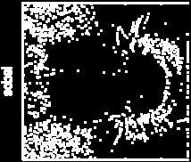
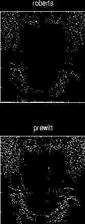
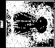
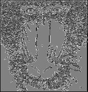
94 Three types of differences generally done are: forward difference = f(x+1) f(x) backward difference = f(x) f(x+1) centre difference = { f(x+1) f(x-1) } / 2 The most common kernels used for the gradient edge detector are the Roberts, Sobel and Prewitt edge operators.

95 Roberts Edge Operator Disadvantage: High sensitivity to noise

96 Prewitt Edge Operator Does some averaging operation to reduce the effect of noise. May be considered as the forward difference operations in all 2-pixel blocks in a 3 x 3 window.

97 Sobel Edge Operator Does some averaging operation to reduce the effect of noise, like the Prewitt operator. May be considered as the forward difference operations in all 2 x 2 blocks in a 3 x 3 window.

98 Gradient Based Edge detection Find f x and f y using a suitable operator. Compute gradient Edge pixels are those for which where T is a suitable threshold

99 Example

100 Second derivative Based For the two-dimensional image, we can consider the orientation-free Laplacian operator as the second derivative. The Laplacian of the image f is given by

101

102 Laplacian Operator Advantages: No thresholding symmetric operation Disadvantages: Noise is more amplified It does not give information about edge orientation

103 Model based edge detection Marr studied the literature on mammalian visual systems and summarized these in five major points: In natural images, features of interest occur at a variety of scales. No single operator can function at all of these scales, so the result of operators at each of many scales should be combined. A natural scene does not appear to consist of diffraction patterns or other wave-like effects, and so some form of local averaging (smoothing) must take place. The optimal smoothing filter that matches the observed requirements of biological vision (smooth and localized in the spatial domain and smooth and band-limited in the frequency domain) is the Gaussian.

104 When a change in intensity (an edge) occurs there is an extreme value in the first derivative or intensity. This corresponds to a zero crossing in the second derivative. The orientation independent differential operator of lowest order is the Laplacian. Based on the five observations an edge detection algorithm is proposed as follows: Convolve the image with a two dimensional Gaussian function. Compute the Laplacian of the convolved image. Edge pixels are those for which there is a zero crossing in the second derivative.

105 LOG Operation Convolving the image with Gaussian and Laplacian operator can be combined into convolution with Laplacian of Gaussian (LoG) operator ( Inverted Maxican Hat) Continuous function and discrete approximation

106 Canny Edge detector Canny s criterion: Minimizing the error of detection. Localization of edge i.e. edge should be detected where it is present in the image. single response corresponding to one edge.

107 Canny Algorithm 1. Smooth the image with Gaussian filter If one wants more detail of the edge, then the variance of the filter is made large.if less detail is required, then the variance is made small. Noise is smoothed out 2. Gradient Operation 3. Non Maximal Suppression: Consider the pixels in the neighborhood of the current pixel. If the gradient magnitude in either of the pixels is greater than the current pixel, mark the current pixel as non edge. 4. Thresholding with hysterisis: mark all pixels with Δf > T H as the edges. mark all pixels with Δf < T L as non edges. a pixel with T L > Δf < T H marked as an edge only if it is connected to a strong edge.

108 Example Canny

109 Edge linking After labeling the edges, we have to link the similar edges to get the object boundary. Two neighboring points (x 1,y 1 ) and (x 2,y 2 ) are linked if

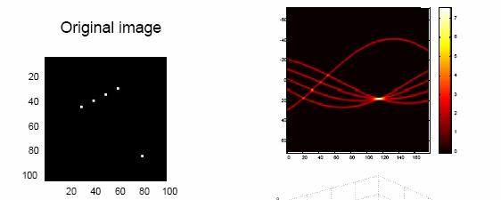
110 Line Detection and Hough transform Many edges can be approximated by straight lines. n n(n 1) 2 For edge pixels, there are possible lines. To find whether a point is closer to a line we have to perform n(n 1) 3 comparisons. Thus, a total of 0( n ) comparisons. 2

111 Hough transform uses parametric representation of a straight line for line detection. y y= mx+ c c ( mc, ) x m

112 y ( x, y ) 1 1 c l 2 c= mx+ y ( xy, ) P l 1 x m The points ( x, y) and ( x1, y1) are mapped to lines l 1and 2 m c respectively in space l 1 and l 2 will intersect at a point P representing the values of the line joining (, y) and ( x, y ). x 1 1 The straight line map of another point collinear with these two l ( mc, ) points will also intersect at P The intersection of multiple lines in the m- c plane will give the (m,c) values of lines in the edge image plane.

113 The transformation is implemented by an accumulator array A, each accumulator corresponding to a quantized value of ( mc, ). The array A is initialized to zero. Corresponding to each edge point for each in the range [ m m ] min,, max c = m x+ y j Increment i find A( i, j) by 1 c N c max ( xy, ), m i M m max m

114 Hough transform algorithm Initialize a 2-D array A of accumulators to zero. For each edge point ( xy, ), find c= mx+ y Increment A( i, j) by 1 Threshold the accumulators: the indices of accumulators with entry greater than a threshold give ( mc, ) values of the lines. Group the edges that belong to each line by traversing each line.

115 m Hough transform variation c and are, in principle, unbounded: cannot handle all situations. Rewrite the line equation as x cos( ) + ysin( ) = θ θ ρ

116 Instead of (, ), we can consider as the parameters α mc ( ρ, θ ) with varying between -90 o and 90 o to M + N for an M N image. p and varying from θ ρ

117 Example

118 Circle detection Other parametric curves like circle ellipse etc. can be detected by Hough transform technique o ( x x ) + ( y y ) = r = constant o For circles of undetermined radius, use 3-d Hough transform for parameters

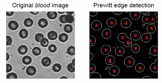
119 Example

120 Compression Basics Today s world is dependent upon a lot of data either stored in a computer or transmitted through a communication system Compression involves reducing the number of bits to represent the data for storing and transmission. Particularly, Image compression is the application of compression on digital images.

121 Storage Requirement Example:One second of digital video without compression requires 720X480X24X25~24.8 MB Example: One 4-minute song: 44100samples per second X16 bits per samplex4x60~20 MB How to store these data efficiently?

122 Band-width requirement The large data rate also means a larger bandwidth requirement for transmission For an available bandwidth of B, the maximum allowable bit-rate is 2B. 2B bits/s can be resolved without ambiguity How to send large amount of data in real-time data through a limited bandwidth channel, say a telephone channel? We have to compress the raw data to store and transmit.

123 Lossless Vs Lossy Compression Lossless A compressed image can be restored without any loss of information Applications Medical images Document images GIS Lossy Perfect reconstruction is not possible but visually useful information is retained Provides large compression Examples Video broadcasting Video conferencing Progressive transmission of images Digital libraries and image databases

124 Encoder and Decoder A digital compression system requires two algorithms: Compression of data at the source (encoding) Decompression at the destination (decoding)

125 What are the principles behind compression? Compression is possible if the signal data contains redundancy. Statistically speaking the data contain highly correlated sample values. Example : Speech data, Image data Temperature and Rainfall Data

126 Types of Redundancy Coding Redundancy Spatial Redundancy Temporal Redundancy Perceptual Redundancy

127 Coding Redundancy Some symbols may be used more often than others In English text, the letter E is far more common than the letter Z. More common symbols are given shorter code-lengths Less common symbols are given bigger code-lengths Coding redundancy is exploited in loss-less coding like Huffman coding

128 Example of Coding Redundancy Morse Code Morse noticed that certain letters occurred more frequently than others. In order to reduce the average time required to send a telegraph message, frequent letters were given shorter symbols. Example: e., a., q and j.--- ( ) ( ) ( ) ( )

129 Spatial Redundancy Neighboring data samples are correlated Given a sample a part of x n 1, x n 2,..., ( ) ( ) x( n) can be predicted if the data are correlated

130 Spatial Correlation: Example

131 Temporal Redundancy In video, same objects may be present in consecutive frames so that objects may be predicted Frame k Frame k+1

132 Perceptual Redundancy Humans are sensible to only limited changes in the amplitude of the signal While choosing the levels of quantization, this fact may be considered Visually lossless means that the degradation is not visible to the human eye

133 Example: Humans are less sensitive to variation of colour 64 levels 32 levels

134 Principle Behind lossless Compression Lossless compression methods work by identifying some frequently occurring symbols in the data, and by representing these symbols in an efficient way. Examples: Run-Length Encoding (RLE). Huffman Coding. Arithmetic coding.

135 Elements of Information Theory Information is a measure of uncertainty A more uncertain (probable) symbol has more information Information of a symbol is related to probability

136 Information Theory (Contd.) Source X is a random variable that takes the symbols x, x,..., x 1 2 with probabilities 1 2 n p, p,..., p The self information or information Ix ( ) is defined as Ix ( ) log i n 1 = 2 p i i

137 Information Theory (Contd.) Suppose a symbol x always occurs. Then p(x) = 1 => I(x) = 0 ( no information) If the base of the logarithm is 2, then the unit of information is called a bit. If p(x) = 1/2, I(x) = -log2(1/2) = 1 bit. Example: Tossing of a fair coin: outcome of this experiment requires one bit to convey the information.

138 Information Theory (Contd.) n 1 ( ) = log / H X p bits symbol i 2 i= 1 pi Average Information content of the source. Measures the uncertainty associated with a source and is called entropy

139 Entropy Introduced by Ludwig Boltzmann His only epitaph S = klnw

140 Properties of Entropy 1. 0 H( X) log 2 ( n) 2. H( X) = log 2 ( n) when all n symbols are equally likely If X is a binary soure with symbols 0 and 1 emitted with probability p and (1- p ) respectively, then 1 1 H( X) = plog 2 ( ) + (1 p) log2 ( ) p 1 p

141 Properties of a Code Codes should be uniquely decodable. Should be instantaneous ( we can decode the code by reading from left to right as soon as the code word is received. Instantaneous codes satisfy the prefix property (no code word is a prefix to any other code). The average codeword length L avg is given by n L = li p avg i i = 1

142 i=1 2 Kraft s Inequality There is an instantaneous binary code with codewords having lengths l, l,... l if and only if n l 2 i For example, there is an instantaneous binary code with lengths 1, 2, 3;,3, since = An example of such a code is 0; 10; 110; 111. There is no instantaneous binary codewith lengths 1, 2, 2, 3, since = > I

143 Shannon s Noiseless Coding theorem Given a discrete memoryless source X with symbols x, x,..., x 1 2 n the average code word length for any instantaneous code is given by L H( X) avg More over there exists at least one code such that L H( X ) + 1 avg

144 Shannon s Noiseless Coding theorem (Contd..) Given a discrete memory less source X with symbols x, x,..., x if we code strings of symbols at a time, 1 2 n the average code word length for any instantaneous code is given by L avg H( X)

145 Example Symbol Probability x x x x H( X ) = 0.125log (1/ 0.125) log (1/ 0.125) log (1/ 0.25) log 2(1/ 0.5) =1.125 bit/symbol 2

146 Example (Contd..) Symbol Probability code x x x x L = 0.125X X X2+ 0.5X1 av = bit/symbol

147 Prefix code and binary tree A prefix code can be represented by a binary tree, each branch being denoted by 0 or 1, emanating from a root node and having n leaf nodes A prefix code is obtained by tracing out branches from the root node to each leaf node.

148 Huffman coding Based on a loss-less statistical method of the 1950s. 0 Creates a probability tree and combines the two lowest probabilities to obtain the code

149 Huffman Coding ( Contd..) Most common data value (with the highest frequency) has the shortest code Huffman table of data value versus code must be sent Time of coding and decoding can be long Typical compression ratios 2:1 3:1

150 Steps in Huffman Coding Arrange symbol probabilities in decreasing order while there is more than one node Merge the two nodes with the smallest probabilities to form a new node with probabilities equal to their sum Arbitrarily assign 1 and 0 to each pair of branches merging in to a node Read sequentially from the root node to the leaf node where the symbol is located p i

151 Run-length coding Looks for sequential pixel values Example: 1 row of an image with the new code below Has reduced the size from 18 bytes to 6 Higher compression ratios when predominantly low frequency information Typical compression ratios of 4:1 to 10:1 Used in Fax machine Used for coding the quantized transform coefficients in a lossy coder

152 Arithmetic coding Codes a sequence of symbols rather than a single symbol at a time A= { a, a, a}; pa ( ) = 0.7, pa ( ) = 0.1, pa ( ) = Now, the sequence has to be coded A single number lying between 0 and 1 is generated, corresponding to all the symbols in the sequence, this number is called tag aa a a Fa ( ) = 0.7, Fa ( ) = 0.8, Fa ( ) =

153 a3 a a a a3 a2 a1 a1 a2 a1 a2 a2 a1 a2 a2 a1 a3 Tag Choose the interval corresponding to the first symbol; the tag will lie in the interval Go on subdividing the subintervals according to the symbol probability The code is the AM of the final subinterval The tag is sent to decoder which has to know the symbol probabilities The decoder will repeat the same procedure to decode the symbols

154 Decoding algorithm for Arithmetic coding 0 0 Initialise k = 0, l = 0, u = 1 Repeat k = k + 1 k 1 * TAG l t = k 1 k 1 u l x such that F ( x ) t < F x ( ) * k X k 1 x k k Update u, l k Until k= size of the sequence Arithmetic code is used to code the symbols in JPEG2000 Disadvantage Assumes data to be stationary, does not consider dynamics of data

155 LZW (Lemple, Ziv and Welch) coding Similar to run-length coding but with some statistical methods similar to Huffman Dynamically builds up a dictionary by both encoders and decoders Examples: Unix command compression Image Compression- Graphics Interchange Format (GIF) Portable document format (PDF)

156 LZW Coding (contd..) Initialize table with single character strings STRING = first input character WHILE not end of input stream CHARACTER = next input character IF STRING + CHARACTER is in the string table STRING = STRING + CHARACTER ELSE output the code for STRING add STRING + CHARACTER to the string table STRING = CHARACTER END WHILE output code for STRING

157 Example Let aabbbaa be the sequence to be encoded; the dictionary will be The output for the given sequence is 11253, which is aabbbaa according to dictionary

158 Lossy Compression Throws away both non-relevant information and a part of relevant information to achieve required compression Usually, involves a series of algorithm-specific transformations to the data, possibly from one domain to another (e.g to frequency domain in Fourier Transform) without storing all the resulting transformation terms and thus, loosing some of the information contained

159 Lossy Compression (contd..) Perceptually unimportant information is discarded. The remaining information is represented efficiently to achieve compression The reconstructed data contains degradations with respect to the original data

160 Example Differential Encoding: Stores the difference between consecutive data samples using a limited number of bits. Discrete Cosine Transform (DCT): Applied to image data. Vector Quantization JPEG (Joint Photographic Experts Group)

161 Fig. Original Lena image, and Reconstructed image from lossy Compression

162 Rate distortion theory Rate distortion theory deals with the problem of representing information allowing a distortion -Less exact representation requires less bits Lossy Coder X Y 2 2 Average distortion ( ) = ( ) E X Y x y p( x) p( y/ x) xy

163 Minimize the bit rate Rate Distortion theory Constraint: Average Distortion between X and Y D source X Lossy Coder Y I( X,Y ) = H(X) H(X Y) Hence: minimize I( X,Y ) under the constraint D

164 Rate Distortion function for a Gaussian source If the source X is a Gaussian random variable, the rate distortion function is given by R( D) = log σ, D< σ 2 D 0, otherwise 2 σ is the variance of Gaussian random variable R(D) D σ 2

165 Rate Distortion Gaussian case presents the worst case of coding For a non Gaussian case, achievable bit error rate is lower than that of Gaussian. If we do not know about anything about the distribution of X, then Gaussian case gives us the pessimistic bound. An increase of 1 bit improves the SNR by about 6 db.

166 Lossy Encoder Fig. A Typical Lossy Signal/Image Encoder Input Data Prediction/ Transformation Quantization Entropy Coding Compressed Data Quantization table Entropy-coding table

167 Differential Encoding [ ] [ ] [ ] Given a sample x n 1, x n 2,..., x n p, a part of xn [ ] can be predicted if the data are correlated. A simple prediction scheme expresses the predicted value as a linear combination of past p samples: p = i i= 1 [ ] [ ] xn ˆ axn i

168 Linear Prediction Coding (LPC) The prediction parameters are estimated using correlation among data The prediction parameters and the prediction error are transmitted a, a... a 1 2 p a, a... a 1 2 p xn ( ) xn ˆ( )

169 LPC (contd..) Variants of LPC (10) are used for coding speech for mobile communication Speech is sampled at 8000 samples per second Frames of 240 samples ( 30 msec of data) are considered for LPC Corresponding to each frame, quantized versions of 10 prediction parameters and approximate prediction errors are transmitted

170 Transform coding Transform coding applies an invertible linear coordinate transformation to the image. Correlated data Transform Less correlated data Most of the energy will be stored in a few transform coefficients Example: Discrete Cosine transform (DCT), Discrete wavelet transform (DWT)

171 Transform selection Transform Merits Demerits KLT Theoretically optimal Data dependent Not fast DFT Very fast Assumes periodicity of data High frequency distortion is more DCT DWT Less high frequency distortion High energy compaction High Energy Compaction Scalabilty because of Gibb s phenomenon Blocking Artifacts Computationally complex Also, DCT is theoretically closer to KLT and implementation wise closer to DFT

172 Discrete Cosine Transform (DCT) Reversible transform, like Fourier Transform N samples of signal f[ m, n], m = 0,1,..., N 1, n = 0,1,..., N 1 DCT is given by ((2m+ 1) u+ ( 2n+ 1) v) N 1 N 1 π Fc ( u, v) = α( u) α( v) f[ m, n]cos, u = 0,1,.. N 1, v= 0,1,.., N 1 m 0 n 0 2N = = 1 1 u = 0 v 0 N = N with α( u) = and α( v) = 2 2 u = 1, 2,.., N -1 v= 1,2,.., N -1 N N

173 DCT (contd..) x DCT Round Threshold IDCT We see that only two DCT coefficients contain most information about the original signal DCT can be easily extended to 2D

174 Block DCT DCT can be efficiently implemented in blocks using FFT and other fast methods. FFT based transform is more computationally efficient if applied in blocks rather than on the entire data. For a data length N and N point FFT, computational complexity is of order Nlog2 If the data is divided into sub-blocks of length then the number of sub-blocks is and the N n N n computational complexity = N n log n 2 = N log n 2 n

175 How to choose block size? Smaller block-size gives more computational efficiency Neighboring blocks will be correlated causing inter block redundancy. If blocks are coded independently, blocking artifact will appear Reconstruction error Block size Beyond 8 8 block size, reduction in error is not significant.

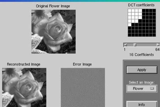
176 4 DCT co-efficients per 8X8 block 8 DCT co-efficients per 8X8 block 16 DCT co-efficients per 8X8 block

177 Quantization Replaces the transform coefficients with lower-precision approximations which can be coded in a more compact form A many-to-one function. Precision is limited by the number of bits available. X= Quant(X)=

178 Quantization (contd..) Information theoretic significance More the variance of the co-efficients, more is the information Estimate the variance of each transform coefficient from given image or determine the variance from the assumed model In the DCT, DC co-efficients: Raleigh distribution AC co-efficients: Generalized Gaussian distribution model

179 Two methods for quantization are zonal coding and threshold coding Zonal coding The co-efficients with more information content (more variance) are retained Threshold coding The co-efficients with higher energy are retained, the rest are assigned zero More adaptive Computationally exhaustive

180 Zonal Coding mask and the number of bits allotted for each coefficient

181 Original image and its DCT Reconstructed image from truncated DCT

182 JPEG Joint Photographic Expert Group A generally used lossy image coding format Allows tradeoff between compression ratio and image quality Can achieve high compression ratio(20+) with almost invisible difference

183 JPEG (contd..) Quantization Table Huffman Table Image 8x8 DCT quantization Huffman Coding Coded Image

184 Baseline JPEG Divide image into blocks of size 8X8. Level shift all 64 pixels values in each 1 block by subtracting, 2 n (where 2 n is the maximum number of gray levels). Compute 2D DCT of a block. Quantize DCT coefficients using a quantization table. Zig-zag scan the quantized DCT coefficients to form 1-D sequence. Code 1-D sequence (AC and DC) usingjpeg Huffman variable length codes.

185 An 8X8 intensity block An image block and DCT

186 Quantization Quantization table

187 Zig-zag scanning

188 Zigzag scanning AC Coefficients (39 zeros)

189 Wavelet Based Compression Recall that DWT is implemented through Row-wise and column-wise filtering and the down-sampling by 2 after each filtering. The approximate image is further decomposed. First and second stages of decomposition are illustrated in the figure below. LL2 HL2 LL1 HL1 HL1 LH2 HH2 LH1 HH LH1 HH 1 First stage 1 Second stage

190 Embedded Tree Image Coding Embedded bit stream: A bit stream at a lower rate is contained in a higher rate bit stream (good for progressive transmission) Embedded Zero-tree Wavelet (EZW) coding algorithm, Shapiro [1993] Set Partitioning In Hierarchical Trees (SPIHT)- based algorithm, Said and Pearlman [1996] EBCOT (Embedded Block Coding with Optimized Truncation) proposed by Taubman in 2000.

191 Tree representation of Wavelet Decomposition

192 EZW EZW scans wavelet coefficients subband by subband. Parents are scanned before any of their children, but only after all neighboring parents have been scanned.

193 EZW coding Each coefficient is compared against the current threshold T. A coefficient is significant if its amplitude is greater then T; such a coefficient is then encoded as Positive significant (PS) Negative significant (NS) Zerotree root (ZTR) is used to signify a coefficient below T, with all its children also below T Isolated zero (IZ) signify a coefficient below T, but with at least one child not below T 2 bits are needed to code this information

194 Successive Approximation quantization Sequentially applies a sequence of thresholds T0,,TN-1 to determine significance Three-level mid-tread quantizer Refined using 2-level quantizer

195 Example Threshold T log2 Cmax lo g2 52 = 2 = 2 = 32

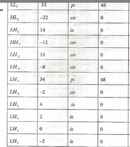
196 Quantization +8-8

197 2 nd Pass

198 JPEG 2000 Not only better efficiency, but also more functionality Superior low bit-rate performance Lossless and lossy compression Multiple resolution Region of interest(roi)

199 JPEG2000 v.s. JPEG JPEG DCT Discrete Cosine Transform 8x8 Quantization Table Huffman Coding Transform Quantization Entropy Coding J2K DWT Discrete Wavelet Transform Quantization for each sub-band Arithmetic Coding

200 JPEG2000 v.s. JPEG low bit-rate performance

201 Video Compression A video sequence consists of a number of pictures, containing a lot of time domain redundancy. This is often exploited to reduce data rates of a video sequence leading to video compression. Motion-compensated frame differencing can be used very effectively to reduce redundant information in sequences Finding corresponding points between frames (i.e., motion estimation) can be difficult because of occlusion, noise, illumination changes, etc Motion vectors (x,y-displacements) are sent

202 Motion-compensated Prediction Reference frame Current frame Predicted frame Error frame

203 Search procedure Reference frame Current frame Best match Search region Current block

204 Search Algorithms Exhaustive Search Three-step search Hierarchical Block Matching

205 Three step search algorithm Search window of ±(2 N 1) pixels is selected (N=3) Search at location (0,0) Set S= 2 N-1 (the step size) Search at eight locations ±S pixels around location (0,0) From the nine locations searched so far, pick the location with smallest Mean Absolute Difference (MAD) and make this the new search origin. Set S=S/2. Repeat stages 4-6 until S=1

206 Three step search algorithm First iteration Minimum at first iteration Second iteration Minimum at second iteration Third iteration Minimum at third iteration

207 Video Compression Standards Two Formal Organizations International Standardization Organization/ International Electro- technical Commission (ISO/IEC) International Telecommunications Organization (ITU-T) ITU-T Standard H.261 (1990) H.263 (1995) ITU-T and ISO/IEC MPEG-2 (1995) H.264/AVC (2003) ISO/IEC standards MPEG-1 (1993) MPEG-4 (1998)

208 Applications And The Bit-rates Supported Standard Application Target bit-rate H.261 Video conferencing and video telephony Px64 kbps 1 P 30 MPEG-1 CD-ROM video applications 1.5Mbps MPEG-2/ H.262 HDTV and DVD Mbps H.263 Transmissions over PSTN networks Up to 64kbps MPEG-4 Multimedia applications 5kbps-50Mbps H.264 Broad cast over cable, Video on demand, Multimedia streaming services 64kbps to 240Mbps

209 MPEG Video Standards Motion Pictures Expert Group Standards for coding video and the associated audio Compression ratio above 100 MPEG 1, MPEG 2, MPEG 4, MPEG 7, MPEG 21.

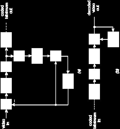
210 MPEG 2 Coder Decoder

211 MPEG 2 Frame Types The MPEG system specifies three types of frames within a sequence: Intra-coded picture (I-frame): Coded independently from all other frames Predictive-coded picture (P-frame): Coded based on a prediction from a past I- or P-frame Bidirectionally predictive coded picture (Bframe): Coded based on a prediction from a past and/or future I- or P-frame(s). Uses the least

212 MPEG 2 GOP structure

213 Image Enhancement Aimed at improving the quality of an image for Better human perception or Better interpretation by machines. Includes both spatial- and frequency-domain techniques: Basic gray level transformations Histogram Modification Average and Median Filtering Frequency domain operations Edge enhancement

214 Image enhancement Input image Enhancement technique Better image Application specific No general theory Can be done in - Spatial domain: Manipulate pixel intensity directly - Frequency domain: Modify the Fourier transform

215 Spatial Domain technique gxy [, ] = T( f[ xy, ]) or s = T( r) X -Simplest case g[.] depends only on the value of f at [ xy, ]; does not depend on the position of the pixel in the image. called brightness transform or point processing

216 Contrast stretching s = T() r

217 Some useful transformations

218 s = 255 r r

219 s = T() r r Enhanced in the range and

220 Thresholding If I[ m, n] > Th Imn [, ] = 255 else Imn [, ] = 0 Th= 120

221 Log transformation Compresses the dynamic range s = clog( r + 1) where c is the scaling factor. Example : Used to display the 2D Fourier Spectrum

222 Log transformation (Contd..)

223 Power law transformation Expands dynamic range s = cr γ where γ c and are positive constants Often referred to as gamma-correction Example : γ =1, Image scaling, same effect as adjusting camera exposure time.

224 Example: Image Display in the monitor Sample Input to Monitor Monitor output

225 Gamma Correction Sample Input Gamma Corrected Input Monitor Output

226 Gamma corrected image Original Image Corrected by γ = 1.5

227 Gamma correction (Contd..)

228 Gray level slicing s s r r

229 Results of slicing in the black and white regions

230 Bit-plane slicing Highlights the contribution of specific bits to image intensity Analyses relative importance of each bit; aids determining the number of quantization levels for each pixel

231 MSB plane Original MSB plane obtained by thresholding at 128

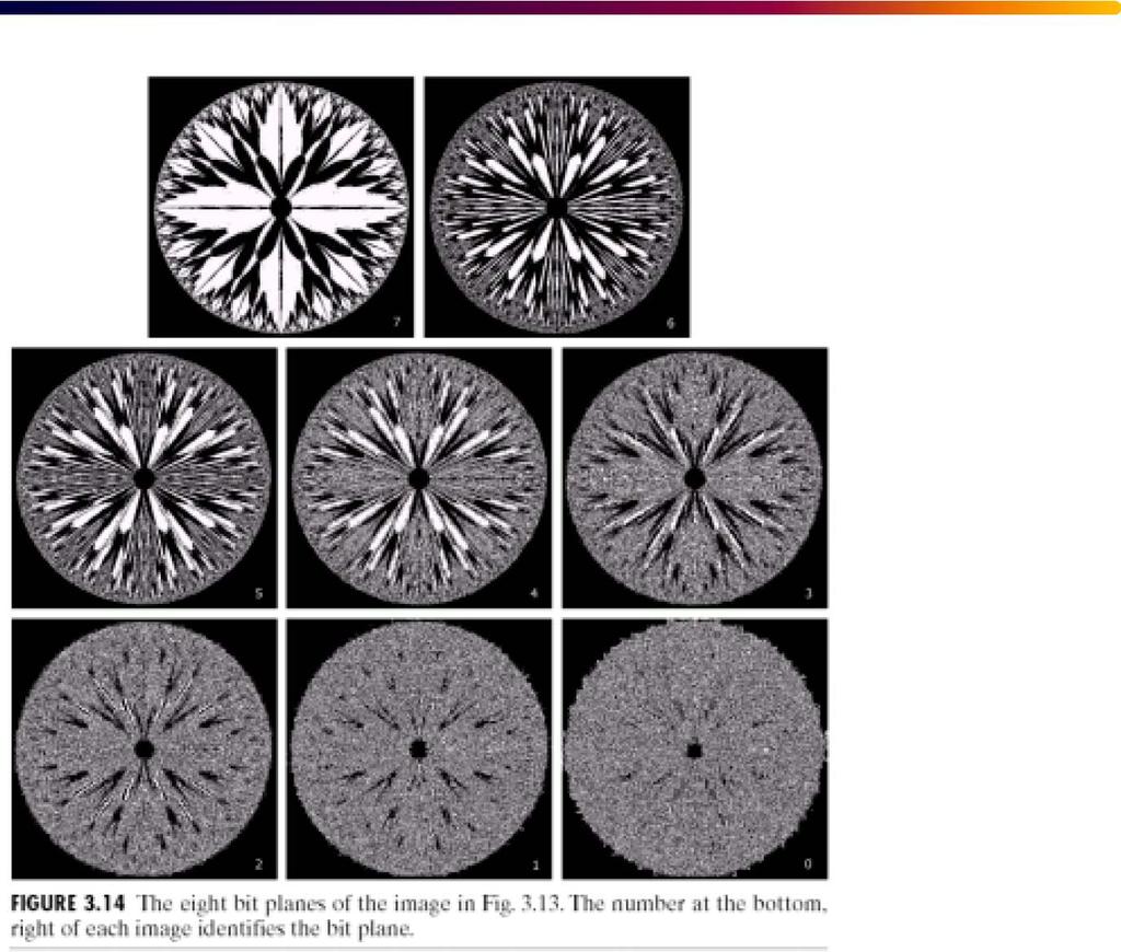
232 Original Image and Eight bit-planes

233 Histogram Processing Includes Histogram Histogram Equalization Histogram specification

234 Histogram r k {0,1,.., L 1} nk pr ( k ) = n n Number of pixels with k gray level r k n Total number of pixels histogram: For B-bit image, initialize 2 B bins with 0 For each pixel x,y If f(x,y)=i, increment bin with index I endif endfor

235 Histogram

236 Low-contrast image Histogram

237 Improved-contrast image Histogram

238 Histogram Equalisation Suppose r represents continuous gray levels0 r 1. Consider a transformation of the form s= T( r) that satisfies the following conditions s= T r is single valued, monotonically increasing in r. (1) ( ) (2) 0 T( r) 1 [ 0,1] T [ 0,1] for 0 r 1 1 Inverse transformation is ( ) T s = r, 0 s 1

239 Histogram Equalisation (contd.) r can be treated as a random variable in [ 0, 1 ] with pdf p r.the pdf of s= T( r) is r ( ) p s ( s) = p ds dr r ( r) r= T 1 ( s) ( ) ( ) Suppose s=t r = p u du,0 r 1 ds then, dr = p r ( r) r 0 r ( r) ( r) pr ps ( s) = 1, 0 s 1 p = r

240 Histogram Equalisation r k k {0,1,.., L 1} nk pr ( k ) = n g = k i= 0 p( r) i The resulting g k needs to be scaled and rounded.

241 Histogram-equalized image image Histogram

242 Histogram-equalized Image

243 Example The following table shows the process of histogram equalization for a 128X128 pixel 3-bit (8- level) image. Gray level r ( ) k nk nk n k ni sk = round X 7 i= 0 n

244 Histogram specification Given an image with a particular histogram, another image which has a specified histogram can be generated and this process is called histogram specification or histogram matching. r 0 z r z ( ) ( ) p r original histogram p z desired histogram ( ) s = pr u du 0 ( ) r = pz w dw ( ) ( ) 1 1 z = G s = G T r

245 Image filtering Image filtering involves Neighbourhood operation taking a filter mask from point to point in an image and perform operations on pixels inside the mask.

246 Linear Filtering he case of linear filtering, the mask is placed over the pixel; the gray value of the image are multiplied with the corresponding mask weights and then added up to give the new value of the pixel. Thus the filtered image g[m,n] is given by gmn [, ] = w f[ m m', n n'] m', n' m' n' Where summations are performed over the window. The filtering window is usually symmetric about the origin so that we can write gmn [, ] = w f[ m+ m', n+ n'] m' n' m', n'

247 Linear Filtering Illustrated

248 Averaging Low-pass filter An example of a linear filter is the averaging low-pass filter. The output I avg of an averaging filter at any pixel is the average of the neighbouring pixels inside the filter mask. It can be given as favg[ mn, ] = wi, j f[ m+ in, + j], where the filter mask is of size m nand fi, j, w i, j are the image pixel values and filter weights respectively. Averaging filter can be used for blurring and noise reduction. Show that averaging low-pass filter reduces noise. Large filtering window means more blurring i j

249 Averaging filter Original Image Noisy Image 1/9 1/9 1/9 1/9 1/9 1/9 1/9 1/9 1/9 Filtered Image

250 Low-pass filter example Filtered with 7X7 averaging mask

251 High-pass filter A highpass filtered image can be computed as the difference between the original and a lowpass filtered version. Highpass = Original Lowpass /9 1/9 1/ /9 1/9 1/ /9 1/9 1/9 = -1/9-1/9-1/9-1/9 8/9-1/9-1/9-1/9-1/9

252 High-pass filtering 1-1/9-1/9-1/9-1/9 8/9-1/9-1/9-1/9-1/9

253 f [ m, n] = Af[ m, n] f [ m, n] A> 1 s Unsharp Masking av = ( A 1) f[ m, n] + f[ m, n] f [ m, n] = ( A 1) f[ m, n] + f [ m, n] high av

254 Verify that median filter is a nonlinear filter. Median filtering The median filter is a nonlinear filter that outputs the median of the data inside a moving window of pre-determined length. This filter is easily implemented and has some attractive properties Useful in eliminating intensity spikes ( salt & pepper noise) Better at preserving edges Works up to 50% of noise corruption

255 Median Sorted data Median= 20, and 255 will be replaced by 20

256 Median Filtering

257 IMAGE TRANSFORMS

258 Image transform Signal data are represented as vectors. The transform changes the basis of the signal space. The transform is usually linear but not shift-invariant. Useful for compact representation of data separation noise and salient image features efficient compression.. A transfom may be orthonormal/unitary or non-orthonormal complete, overcomplete, or undercomplete. applied to image blocks or the whole image..

259 DATA 1D TRANSFORM

260 UNITARY TRANSFORM

261 Unitary transform and basis t t... t 0,0 0,1 0, N 1 t t... t 1,0 1,1 1, N 1 T = : t t... t N 1,0 N 1,1 N 1, N 1 Then T 1 * * * t t... t 0,0 1,0 N 1,0 * * * t t... t 0,1 1,1 1, N 1 = : * * * t t... t N 1,0 N 1,1 N 1, N 1

262 Unitary transform and basis (Contd..) Therefore, * * * f[0] t t... t 0,0 1,0 N 1,0 F[0] * * * f[1] t t... t 0,1 1,1 1, N 1 F[1] : = : : * * * f[ N 1] t t... t F[ N 1] 0, N 1 1, N 1 N 1, N 1 * * * t0,0 t1,0 tn 1,0 * * * t0,1 t1,1 tn 1,1 = F[0] : + F[1] : +... F[1] : * * * t t t N 1,0 1, N 1 N 1, N 1 Since the columns of T 1 are independent, they form a basis for the N- dimensional space

263 Examples of Unitary Transform 2D DFT Other Examples : DCT (Discrete Cosine Transform) DST (Discrete Sine Transform) DHT (Discrete Hardmard Transform) KLT (Karhunen Loeve Transform)

264 Properties of Unitary Transform 1. The rows of T form an orthogonal basis for the N- dimensional complex space. 2. All the eigen vectors of T have unit magnitude Tf = λf

265 3. Parseval s theorem: T is energy preserving transformation, because it is an unitary transform which preserves energy F*' F = energy in transform domain f*' f = energy in data domain F*' F = [Tf]*' Tf = f*' T*' Tf = f*' I f = f*' f 4. Unitary transform is a length and distance preserving transform. 5. Energy is conserved, but often will be unevenly distributedamong coefficients.

266 Decorrelating property makes the data sequence uncorrelated. useful for compression Let f = [ f[0],,f[n-1] ] T be data vector, = Covariance matrix = Covariance matrix of transformation Diagonal elements of C Ft variance, off-diagonal elements of C Ft Covariance Perfect Decorrelation off-diagonal elements are zero.

267 2D CASE

268 Separable Property

269 Matrix representation If we consider separable, unitary and symmetric transform. = N 1 N 1 f n n t k n t n k n = n = [, ][, ][, ] 2 1 Thus we can write

270 2D Separable, unitary and symmetric transforms have following properties: i. Energy preserving ii. iii. iv. Distance preserving Energy compaction Other properties specific to particular transforms..

271 Karhunen Loeve (KL) transform Let f = [ f[0],,f[n-1] ] T be data vector, = Covariance matrix C f can be diagonalised by UCU f =Λ Λ where is diagonal matrix formed by eigen values U is matrix formed by eigen vectors as columns Transform matrix of KL transform is T = U

272 KL Transform KL transform is F KLT=T KLT(f-μ f) E(F KLT ) = 0

273 KL Taransform Covariance Matrix C FKLT is

274 For KLT eigen values are arranged in descending order and the transformation matrix is formed by considering the eigen vectors in order of the eigen values. Reconstructed value is Suppose we want to retain only k- transform coefficients we will retain the transformation matrix formed by the k largest eigen vectors. Principal Component Analysis (PCA) Linear combination of largest principal eigen vectors.

275 KLT Illustrated F 2 F 1

276 KL transform Mean square error of approximation is E( f-fˆ)( f-fˆ) = Energy of f Energy of f N 1 J 1 = λ λ = i= 0 i i= 0 N 1 i= j Mean square error is minimum over all affine transforms. Transform matrix is data dependent so computationally extensive. λ i i

277 1D-DCT Let f = [ f[0],,f[n-1] ] T be data vector 1D-DCT of data vector f and its IDCT are where

278 The transformation can be written as F = T C f where T C is transformation matrix with elements DCT is a real transform. T C is orthogonal transform T C T C = I so T C -1 = T C

279 f ( n ) = f ( n ), n N 1 = 0, N < 1 n 2 N 1 Relation with DFT DCT : j2π 1 nk jπ k N FC() k α()re k al = f() ne 2N e 2N n = 0 Let f () n = f [ n], for n= 0,1,..., N 1 0, otherwise DCT of f() n is given by j2π 2 1 nk jπ k N FC() k α()re k al = f () ne 2N e 2N n = 0

280 Another interpretation (21),fN = N < Extend the data symmetrically about n=n-1 so that f () n = DFT of f () n is given by F fn [ ], for n= 0,1,..., N 1 f (2N 1 n), n= N, N+ 1,...,2N 1 N 1 = n = 0 ( k) f( n) e + f(2n 1 n) e j2π j2π nk k(2n 1 n) ' 2N 2N j2 j j2 j N 1 π nk π nk πnk π nk = f n e 2N e 2N + e 2N e 2N j2π nk e 2N () n = 0 jπ nk N 1 ()cos( k e N f n π = (2n+ 1) ) 2N n = 0 N 1 ( ) ( ) ()cos( π k F k = α k (2n 1) c f n + ) n = 0 2N jπnk jπnk N e N en n = 0 = = α( k) + e jπ nk N α( kf ) '( k) 1 f()cos( n π k (2n 1) ) 2N

281 Interpretation of DCT with DFT DCT

282 2D-DCT f(, nn) The 2D DCT of is 1 2 2D DCT can be implemented from 1D DCT by Performing 1D DCT column wise Then performing 1D DCT row wise

283 DCT is close to KLT Firstly, DCT of basis vectors will be eigen vectors of triangular matrix Secondly, a first order markov process with correlation coefficient ρ has a covariance matrix

284 If ρ is close to 1 then Therefore for a Markov first order process with ρ close to 1 DCT is close to KLT. Because of closeness to KLT, energy compaction, data decorrelation and ease of computation DCT is used in many applications.

285 Matrices Many image processing operations are efficiently implemented in terms of matrices Particularly, many linear transforms are used Simple example: colur transformation Y R I = G Q B

286 Matrix representation of linear operations [ ] [ ] [ ] Let x 0, x 1,..., x N 1 be N data samples. These data points can be represented by a vector Consider a transformation [ 0] [] 1 y y... y N N 1 [ ] [ ] j= 0 Denoting we get where [ -1] y= y=ax x 0 x 1 x= x N-1 yn= ax j, n= 0,1,..., N 1 nj A a a a... a a a a... a a a a... a 0,0 0,1 0,2 0, N 1 1,0 1,1 1,2 1, N 1 2,0 2,1 2,2 2, N 1 =.. a a a... a N 1,0 N 1,1 N 1,2 N 1, N 1

287 Example: Discrete Fourier transform N 1 [ ] [ ] xk = n= 0 xne 2π i nk N k=0,1,...n-1 [ ] [] 1 X x 0 2π 2 π ( 1) X j j N N N 1 e... e x[] 1.. = π 2π. j ( N 1 ) j ( N 1) ( N 1) N N X[ N 1] 1 e... e xn [ 1] [ ]

288 Example: Rotation operation y ( x, y ) θ r θ 0 r ( xy, ) x = xcosθ ysinθ x y = xsinθ + ycosθ x cos θ sinθ x = y sin θ cosθ y

289 Transpose of a matrix: Matrices - Basic Definitions T A A Symmetric Matrix: = T A A *T Hermitian Matrix: = A Example: A 1 i 1 i -i 1 -i 1 T =, A = 1 A A= I A Inverse of a Matrix: for a non singular matrix

290 Unitary Matrix A 1 T A matrix of complex elements is called unitary if A = A A Example = j j j j

291 Orthogonal Matrix For an orthogonal matrix A A 1 T = A Real-valued unitary matrices are orthogonal Example: Rotation operation y = xsinθ + ycosθ x = xcosθ ysinθ A cosθ -sinθ = sin θ cosθ 1 cos θ sin θ A = = -sin θ cos θ A T

292 Example Is the following matrix orthogonal?

293 Toeplitz Matrix A matrix is called Toeplitz if the diagonal contains the same element, each of the sub-diagonals contains the same element and each of the super-diagonals contains the same element. The system matrix corresponding to linear convolution of two sequences is a Toeplitz matrix. The autocorrelation matrix of a wide-sense stationary process is Toeplitz. Example A a0,0 a0,1... a0, N 1 a a a... a a a a... a 1,0 0,0 0,1 1, N 1 2,0 1,0 0,0 2, N 1 =.. a a.. a a N 1,0 N 1,1 1,0 0,0

294 Circulant Matrix A matrix is called a Circulant Matrix if each row is obtained by the circular shift of the previous row. a0,0 a0,1... a0, N 1 a0, N 1 a0,0 a0,1... a0, N 2 a0, N 2 a0, N 1 a0,0... a 0, N 3 Example A =.. a0,1 a0, a0, N 1 a 0,0 The system matrix corresponding to circular convolution of two sequences is a circulant matrix.

295 Eigen Values and Eigen Vectors A λ Ax = λx λ x If is a square matrix and is a scalar such that then is the eigen value and is the corresponding eigen vector. Thus the eigen vectors are invariant in direction under an operation by a matrix. Example: Rotation operation with x 0-1 x = y 1 0 y A θ = = 1 0 then then No real eigen values and eigen vectors exist. Now consider Rotation operation with θ =180 so that each vector is invariant under rotation by then A -1 0 = 0-1

296 Morphological Image Processing Basically, a filtering operation. Set-theoretic operations are used for image processing applications. Such operations are simple and fast. In normal image filtering, we have an image and filtering is done through the convolution mask. In morphological image filtering, the same is done through the structuring element

297 Binary Morphology Basics Image plane is represented by a set {( x, y) ( x, y) Z 2 } A binary object is represented by A= (, x y) I(, x y) = 1 { } in Binary Image Morphology Background c A = (, x y) I(, x y) = 0 In Gray-scale Morphology, { } { 2 (,, ) (, ) Z, (, ) } A = x y z x y I x y = z A The value of z gives the gray value and (x, y) gives the gray point.

298 Structuring element It is similar to mask in convolution It is used to operate on the object image A A Structuring element A Entire image B

299 B Bˆ Reflection and Translation operations (1) Reflection Operation: Reflection of is given by A A ˆ = (, xy ) ( x, y ) A { } (2) Translation Operation: Translation of by an amount is given by A = a + x a A ( ) { } x A x x

300 Binary image morphology operations a. Dilation operation b. Erosion operation c. Closing operation d. Opening operation e. Hit or Miss transform

301 Dilation operation Given a set A and the structuring element B, we define dilation of A with B as { ( ˆ ) } A B = x A B x A A A B B

302 Why dilation? If there is a very small object, say (hole) inside the object A, then this unfilled hole inside the object is filled up. Small disconnected regions outside the boundary may be connected by dilation. Irregular boundary may be smoothened out.

303 Properties of Dilation A B = B A A ( B C) = ( A B) C Dilation is commutative Dilation is associative ( A B) x = A x B 3. Dilation is translation invariant

304 Erosion operation Erosion of A with B is given by, { } AΘ B = x B A x A B Here, structuring element B should be completely inside the object A.

305 Why Erosion? 1. Two nearly connected regions will be separated by erosion operation. 1. Shrinks the size of the objects 3. Removes peninsulas and small objects. 4. Boundary may be smoothened

306 Properties of Erosion AΘ B = A ΘB 1. Erosion is translation invariant ( ) x x 2. Erosion is not commutative 3. Erosion is not associative ( A B) Θ BΘA ( AΘB) Θ C= AΘ( B C) Dilation and erosion are dual operations in the sense that, ( ) C C AΘ B = A Bˆ ( ˆ ) C C A B = A ΘB

307 Opening and Closing operation Dilation, and Erosion changes size By opening and closing operations, irregular boundaries may be smoothened without changing the overall size of the object Original Dilated

308 Closing operation Dilation, followed by Erosion A B = ( A B) ΘB After Dilation operation, the size of the object is increased and it is brought back to the original size by erosion operation Closing Object A Structuring element B By closing operation, irregular boundaries may be smoothened depending upon the structural element

309 Example Original Dilated Closed

310 Opening operation Erosion, followed by Dilation A o B = ( AΘB) B Opens the weak links between the nearby objects Smoothens the irregular boundary In all operations, performance depends upon the structuring element and is applied to binary images. Example: Edge detection

311 Example A={(1,0), (1,1), (1,2),(1,3), (0,3)} B={(0.0), (1.0)} A B = ={(1,0), (1,1), (1,2),(1,3), (0,3),(2,0), (2,1), (2,2),(2,3)} AΘ B = {(1,3), (0,3)} We can similarly do other morphological operations

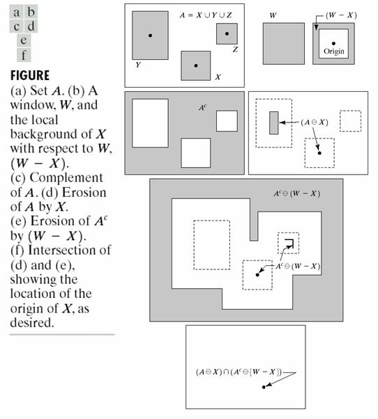
312 The transform is given by Hit or Miss transform ( ) ( C ) 1 2 A B= AΘB A ΘB ( ) ( ˆ ) 1 2 A B= AΘB A B C where B 2 = W B1 W is the window around the structuring element The main aim of this transform is pattern matching

313 Procedure for Hit-or-Miss Transform W Object A Structuring element B1 C A B2=W-B1 After B2 is obtained, find ( ) ( C ) 1 2 A B= AΘB A ΘB

314 Example In a text, how many F s are present? Structuring element or The structuring element will match both E & F.In such cases, background is also considered for pattern matching Hit or miss transform will match F only

315 Example

316 Applications of binary morphology operations 1. Boundary extraction β ( A ) = A ( AΘB)

317 Applications of binary morphology operations 2. Region filling (a)starts with a pixel inside the unfilled region (b)select a proper structuring element B and perform X = X B A n ( ) n 1 X 0 Repeat this operation n n 1 X C = X After getting X n find A X n to get the filled region

318 3. Thinning operation This gives the image as single pixel width line object Thinning object skeletonizing

319 3. Thinning operation Thinning and skeletonizing are impact operations Thinning operator A B = A ( A B)

320 B 1 Original image A 1 s 0 s Go on matching until exact matching is achieved Now, consider another structuring element 2 Then, the thinning operation is B ( ) ( 1) A B= A A B A A B B 1 2 In this manner, we can do hit or miss with structuring elements to get ultimately thinned object

321 Skeletonizing The skeleton is given by the operation K SA ( ) = S( A) where k= 0 k S ( A) = ( AΘkB) ( AΘkB) ob k U

322 Gray-scale morphology.generalization of binary morphology to gray-level images Max and Min operations are used in place of OR and AND Nonlinear operation The generalization only applies to flat structuring elements..

323 Gray scale morphological operations f x, y ( ) Object (intensity surface) bxy (, ) Structuring element (will also have an intensity surface) Domain of f ( x, y ) Domain of bxy (, ) D f Db Domain of object Domain of structuring element

324 Dilation at a point (s,t) of f with b ( )(, ) max (, ) (, ),,,(, ) { } f b s t = f s x t y + b x y s x t y D x y D It can also be written like in convolution f ( x, y) + b( s x, t y) Here, mask is rotated by 180 degree and placed over the object; from overlapping pixels, maximum value is considered. Since it is a maxima operation, darker regions become bright Applications 1. Pepper noise can be removed 2. Size of the image is also changed. f b

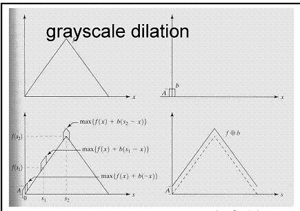
325 Dilation Illustrated

326 Dilation Result

327 Erosion operation ( )(, ) min (, ) (, ),(, ),(, ) { } f Θ b s t = f s+ xt+ y bxy s+ xt+ y D x y D It is a minimum operation and hence, bright details will be reduced. Application: Salt noise is removed f b We can erose and dilate with a flat structuring element

328 Erosion Result

329 Closing operation f b= ( f b) Θb Removes pepper noise Keeps intensity approximately constant Keeps brightness features

330 Opening operation f ob= ( fθb) b Removes salt noise Brightness level is maintained Dark features are preserved

331 Opening and Closing illustration

332 Closing and Opening results Original image closing opening

333 Duality Gray-scale dilation and erosion are duals with respect to function complementation and reflection c f Θ b s, t = f bˆ s, t ( ) ( ) ( c )( ) Gray-scale opening and closing are duals with respect to function complementation and reflection ( ) c c f b = f obˆ

334 Smoothing Opening followed by closing Removes bright and dark artifacts, noise

335 Morphological gradient g = f b fθb Subtract the Eroded image from the dilated image Similar to boundary detection in the case of binary image Direction Independent

336 Probability and Random processes Probability and random processes are widely used in image processing. For example in Image enhancement Image coding Texture Image processing Pattern matching Two ways of applications: (a) The intensity levels can be considered as the values of a discrete random variable with a probability mass function. (b) Image intensity as two-dimensional random process

337 The following figure shows an image and its histogram We can use this distribution of grey levels to extract meaningful information about the image. Example: Coding application and segmentation application

338 We may also model the analog image as a continuous random variable

339 Probability concepts Random Experiment: An experiment is a random experiment if its outcome cannot be predicted precisely. One out of a number of outcomes is possible in a random experiment. A single performance of the random experiment is called a trial. 2. Sample Space: The sample space is the collection of all possible outcomes of a random experiment. The elements of are called sample points. 3. Event: An event A is a subset of the sample space such that probability can be assigned to it.

340 Probability Definitions Classical definition of probability) Consider a random experiment with a finite number of outcomes. If all the outcomes of the experiment are equally likely, the probability of an event is defined by N A N A P( A) = N Where is the number of outcomes favourable to A. Example A fair die is rolled once. What is the probability of getting a 6? Here S = {'1', '2 ', '3', '4 ', '5', '6 '} and 1 P( A) =. 6 A = { '6'}.

341 Relative Frequency Definition If an experiment is repeated n times under similar conditions and the event A occurs in times, then n A na PA ( ) = Lim n n Example: Suppose a die is rolled 500 times. The following table shows the frequency each face. Face Frequency Then 78 1 PA= ( ) 500 6

342 PX Image Intensity as a Random Variable x 0 1. L-1 ( x) p 0. p p 1 L 1 For each gray level i, fi hi [] = N where f i is the number of pixels with intensity i. The probability is estimated from the histogram of the image.

343 Some Important Properties Probability that either A or B or both occurs is given by PAUB ( ) = PA ( ) + PB ( ) PA ( B) PS ( ) = 1 If A and B are mutually exclusive or disjoint, then PA ( B) = 0

344 Conditional Probability the conditional probability of B given A denoted by is defined by P(B/A) P(B/A) = Similarly PA ( / B) = N N A B A N A B = N N A N PA ( B) = PA ( ) PA ( B) PB ( )

345 Independent events Two events are called independent if the probability of occurrence of one event does not affect the probability of occurrence of the other. Thus the events A and B are independent if and only if or PB ( / A) = PB ( ) PA ( / B) = PA ( ) and hence P( A B) = P( A) P( B)

346 Random variable A random variable associates the points in the sample space with real numbers. Consider the probability space and function mapping the sample space into the real line. Real line S Domain of X Figure Random variable X Range of X

347 Probability Distribution Function The probability P({ X x}) = P({ s X( s) x, s S}) is called the probability distribution function (also called the cumulative distribution function abbreviated as CDF) of X and denoted by FX ( x ). Thus (, x], F ( x) = P({ X x}) X FX ( x) Value of the random variable Properties of Distribution Function Random variable 0 F ( x) 1 X F X (x) is a non-decreasing function of X. Thus, x 1 < x 2 FX x 1 < FX x 2 F ( ) = X 0, then ( ) ( ) F ( ) = 1 X P x1 < X x2 = FX x2 FX x1 ({ }) ( ) ( )

348 Example Suppose S = { H, T} and X: S is defined by XH= ( ) 1 and XT ( ) = 1. Therefore, X is a random variable that can take values 1 with probability 1 2 and -1 with probability 1 2. S H 1 T -1 F () X x X o x x

349 If F X (x) is differentiable, the probability density function (pdf) of, f x is defined as by ( ), X f d ( x) FX ( x) dx X = Properties of the Probability Density Function fx ( x) 0. Probability Density Function This follows from the fact that F ( x) is a non-decreasing function X X denoted x FX( x) = fx( u) du f X ( x) f X ( x) dx = 1 P ( x1 < X x2 ) = f x 2 x 1 X ( x) dx x 0 x +Δ x 0 0 P({ x < X x +Δx }) f ( x ) Δx X 0 0 x

350 Example Uniform Random Variable 1 fx ( x) = b- a 0 a x b otherwise Gaussian or Normal Random Variable 1 fx ( x) = e 2πσX, < x < 2 1 x μ X 2 σ X

351 Functions of a Random variable Let X be a random variable and g (.) be a function of X. Then Y = g( X ) is a random variable. We are interested to find the pdf of Y. For example, suppose X represents the random voltage input to a full-wave rectifier. Then the rectifier output Y is given by Y = X. We have to find the probability description of the random variable Y. We consider the case when g( X ) is a monotonically increasing or monotonically decreasing function. Here fx( x) fx( x) fy ( y) = = dy g ( x) x= g 1 ( y) dx Example: Probability density function of a linear function of a random variable Suppose Y = ax + b, a> 0. y b dy Then x = and = a a dx y b f ( ) f ( ) X X x fy ( y) = = a dy a dx

352 EXPECTATION AND MOMENTS OF A RANDOM VARIABLE The expectation operation extracts a few parameters of a random variable and provides a summary description of the random variable in terms of these parameters. The expected value or mean of a continuous random variable X is defined by μ X = EX = N i= 1 xf X xp ( x) dx for a continuous RV i X i ( x) for a discrete RV Generally for any function g( X ) of a RV X Particularly, Mean-square value Variance EY = Eg( X ) = g( x) f ( x) dx 2 2 = X X X X X X E X x f (x)dx σ =E(X-μ ) = (x- μ ) f (x)dx

353 Multiple Random variables In many applications we have to deal with many random variables. For example, the noise affecting the R B channels of colour video may be represented by three random variables. In such situations, it is conven to define the vector-valued random variables where each component of the vector is a random variable. Joint CDF of n random variables Consider nrandom variables X1, X2,.., X n defined on the same sample space. We define the random vect as, X 1 X 2 X =.. X n A particular value of the random vector Xis denoted by x1 x x xn 2 =. The CDF of the random vector X is defined as follows F ( x, x,.. x ) = F (x) X, X,.., X 1 2 n X 1 2 n = P({ X x, X x,.. X x }) n n

354 Multiple random variables If X is a continuous random vector, that is, F ( x, x,.. x ) is continuous in each of X, X,.. X 1 2 n 1 2 n its arguments, then X can be specified by the joint probability density function n f (x) = f ( x, x,.. x ) = F ( x, x,.. x ) X X, X,.. X 1 2 n... X, X,.. X 1 2 n 1 2 n x x x 1 2 n 1 2 n We also define the following important parameters. The mean vector of X, denoted by μ, is defined as X μ X E( X) E( X ) 1 E( X ) E( X ) n μ X 1 μ μ X n 2 = = X 2 =

355 Multiple Random Variables Similarly for each ( i, j) i= 1,2,.., n, j = 1,2,.., n we can define the covariance Cov( X, X ) = E( X μ )( X μ ) = EX X μ μ and the correlation coefficient ρ X, X i j i j i X j X i j X X Cov( X i, X j) = σ σ X i X j i j i j All the possible covariances and variances can be represented in terms of a matrix called the covariance matrix C defined by C = E( X μ )( X μ ) X X X var( X1) cov( X1, X2) cov( X1, Xn) cov( X, X ) var( X ). cov( X, X ) cov( Xn, X1) cov( Xn, X2) var( Xn) n = X

356 Multi-dimensional Gaussian Suppose for any positive integer, n 1 2 X, X,..., X n represent n jointly random variables. These random variables are called jointly Gaussian if the random variables X, X,..., X 1 2 n have joint probability density function given by f ( x, x,... x ) = X, X,..., X 1 2 n 1 2 n e ( π ) 1 ( )' 1 X μx C X ( X μx ) 2 n 2 det( ) C X where C = E( X μ )( X μ )' is the covariance matrix and X X X [ 1 2 ] μ = E( X) = E( X ), E( X )... E( X n ) ' is the vector formed by the means of the random X variables.

357 Example 2D Gaussian Two random variables X and Y are called jointly Gaussian if their joint density function is + 1 fx, Y( x, y) = e 2πσ σ 1 ρ 2 X Y X, Y ( x μ ) 2 ( x μ )( y μ ) ( y μ ) 2 1 X 2 X Y Y 2(1 2 ρ ) 2 XY ρ σ σ 2 X, Y σ X X Y σ Y - < x<, - < y< The joint pdf is determined by 5 parameters means μ and μ X Y variances 2 2 σ and σ X Y correlation coefficient ρ, X Y.

358 Karhunen-Loe ve transform (KLT) X [ 1] X [ 2] Let a random vector X be given as and characterized by mean μ and X =.. X[ N ] auto co-variance matrix C ( )( ) ' X = E X μx X μx. is a positive definite matrix. This matrix can be digitalized as C X λ λ2.. T φ C = Xφ λn Where λ1, λ2... λnare the eigen values of the matrix C and φ X is the matrix formed with the eigen vectors as its columns. ( ) T Consider the transformation Y = φ X μ x. Then, CYwill be a diagonal matrix and the transformation is called the Karhunen Loe ve transform (KLT). x

359 Random Process X(, t s 3) S s 3 X(, t s 2) s 2 s 1 X(, t s 1) Recall that a random variable maps each sample point in the sample space to a point in the real line. A random process maps each sample point to a waveform. A random process is thus a function of t and s. The random process X(t,s) is usually denoted by X(t). Discrete time random process X[n].

360 The discrete random process dimensional variable n. is a function of one- Some important parameters of a random process are: Mean: Variance: [ n] EX[ n] μ = σ { X[ n] } [ n] = E X n μ[ n] ( [ ] ) 2 2 Auto correlation: Auto covariance: X X [, ] = [ ] [ ] ( )( [ ] μ[ ]) [, ] [ ] μ[ ] ( ) R nm E X n X m C n m = E X n n X m m

361 Wide sense stationary (WSS) random process For WSS process the Mean [ ] = = constant EX n μ X and the autocorrelation function [ ] R mn, = EXmXn [ ] [ ] X is a function of the lag X [ n], n m only. X [ n], We denote the autocorrelation function of a WSS process at lag k by Autocorrelation function R [ ] is even symmetric with a maximum at k=0. X k

362 Mean vector: Matrix Representation We can represent N samples by an N-dimensional random vector [ 1] [ 2] X X X =.. X [ N ] μx [ ] [ ] [ ] [ ] EX 1 μx 1 EX 2 μx 2 = EX =. =... EX [ N ] μx [ N ] Autocorrelation matrix: Auto covariance matrix: RX = E XX C =E X-μ ( )( X-μ ) x X X Check that R and C are symmetric Toeplitz matrix X X

363 Frequency-domain Representation A host of tools are available to study a WSS process. Particularly, we may have the frequency domain representation of a WSS process in terms of the power spectral density (PSD) given by j k SX( ω) = RX[ k] e ω k = ( ω) The autocorrelation function is obtained by the inverse transform of X as given by S π 1 [ ] jωk RX k = SX( ω) e dω 2 π π

364 Gaussian random process A random process { X [ n] } is called a Gaussian process if for any N, the joint density function is given by, 1 f x x x x = e (,,,..., ) X[1], X[2],..., X[ N] N N ( 2π ) det( C x ) 1 ( )' -1 x μx CX ( x μx ) 2 where the vecors and the matrices are as interpreted earlier.

365 Markov process { Xn [ ]} is a random process with discrete state.i.e. X[ n] can take the one of discrete values x 0, x 1, x 2,... x L 1with certain probabilities as shown below. State: x0, x1, x2,... x L 1 Probabilities: p0, p1, p2,..., pl 1 L { X[ n]} is called first-order Markov if { [ ] [ ] [ ] } [ ] [ ] Thus for a first-order Markov process, the current state depends on the immediate past. Similarly, { X[ n]} is called p th-order Markov if A first-order Markov process is generally called a Markov process. { } P( X n = x X n 1 = x, X n 2 = x,... ) = P( X n = x X n 1 = x ) n n 1 n 2 n n 1 ({ [ ] = n [ 1 ] = n 1, [ 2 ] = n 2,... }) [ ] [ 1 ], [ 2 ],..., [ ] P X n x X n x X n x ({ n n 1 n 2 n p} ) = P X n = x X n = x X n = x X n p = x

366 Random field A two dimensional random sequence { Xmn [, ]} is called a random field. For a random field { X [ mn, ]}, we can define the mean and the autocorrelation functions as follows: Mean: [ ] EX m, n = μ[ m, n] Autocorrelation: [ ] R m, n, m, n = EX[ m, n] X[ m, n ] X A random field { X[ mn, ]} is called a wide-sense stationary (WSS) or homogeneous random field if R [ mnm,,, n ] is a function of the lags [ m m, n n ]. X Thus, for a WSS random field { [, ]}, the autocorrelation function RX k, l can be defined by [ ] Xmn [ ] R kl, = EXmnXm [, ] [ + kn, + l) X = EX[ m+ kn, + lxmn ] [, ] X [, ] = R k l

367 A random field { Xmn [, ]} is called an isotropic random field if { [, ]} A random field is called a separable random field if R can be X m, n separated as R m, n = R m R n Two-dimensional power spectral density We have the frequency domain representation of a WSS random field in terms of the two-dimensional power spectral density given by j( uk + vl ) S ( u, v) R [ k, l] e The autocorrelation function R [ kl, ] is given by X 2 2 [,,, ] is a function of the distance ( ) + ( ) R m n m n m m n n Xmn [ ] [ ] [ ] [ ] X X X { f [ mn, ]} 1 2 f A random field is called a Markov random field if the current state at a location depends only on the states of the neighboring locations. X X = l= k= π π 1 = 2 4π π π juk ( + vl) [, ] (, ) R k l S u v e dudv X X

368 Segmentation Divide the image into homogenous segments. Homogeneity may be in terms of (1) Gray values (within a region the gray values don t vary much ) Ex: gray level of characters is < gray level of background colour (2) Texture : some type of repetitive statistical uniformity (3) Shape (4) Motion (used in video segmentation)

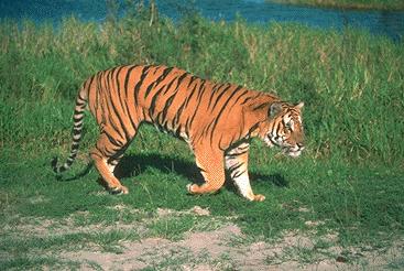
369 Example

370 Segmentation based on texture Segmentation based on Colour

371 Application Optical character recognition Industrial inspection Robotics Determining the microstructure of biological, metallurgical specimens Remote sensing Astronomical applications Medical image segmentation Object based compression techniques (MPEG 4) Related area in object representation

372 Histogram-based segmentation Region-based segmentation Edge detection Region growing Region splitting and merging. Clustering K-means Mean shift Main approaches Motion segmentation

373 Example: Text and Background Problem: we are given an image of a paper, and we would like to extract the text from the image. Thresholding: define a threshold Th such that If I(x,y) < Th Then object(character) Else background (paper) How do we determine the threshold? Just choose 128 as a threshold (problematic for dark images) Use the median/mean (both are not good, as most of the paper is white)

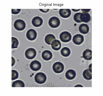
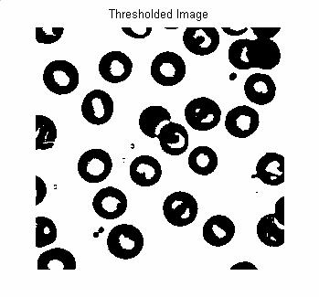
374 Example

375 Histogram-based Threshold Assumption Regions are distinct in terms of gray level range Frequency Gray level

376 Histogram-based threshold Compute the gray level histogram of the image. Find two clusters : black and white. Minimizing the L 2 error: Select initial estimate T Segment the image using T. Compute the average gray level of each segment m b,m w Compute a new threshold value: T = ½ (m b +m w ) Continue until convergence. We are already familiar with this algorithm!

377 Problems with this approach Noise Many holes and discontinuities in the segmentation. Changes in the illumination We do not use spatial information. Some of the problems can be solved using image processing techniques. For example, we can enhance the result using morphological operations. Yet How can we overcome the changes in the illumination?

378 Adaptive Thresholding Divide the image into sub-images. Assume that the illumination in each sub-images is constant. Use a different threshold for each sub-image. Alternatively use a running window (and use the threshold of the window only for the central pixel ) Problems: Rapid illumination changes. Regions without text: we can try to recognize that these regions is unimodal.

379 Optimal Thresholding We may use probability based approach. Intensity histogram is a mixture of Gaussian distribution. Normalized histogram = sum of two Gaussian with different mean and variance. Identify the Gaussian Decide the threshold

380 Region-based segmentation We would like to use spatial information. We assume that neighboring pixels tend to belong to the same segment (not always true) Edge detection: Looking for the boundaries of the segments. Problem: Edges usually do not determine close contours. We can try to do it with edge linking

381 Region-based segmentation Basic Formulation Let R represent the entire image region. Segmentation: Partitioning R into n subgroups R i s.t: a) U R i = R i b) R i is a connected region c) R I i R j = φ d) P( Ri U R j ) = False e) P( R i ) = True P is the partition predicate Partition should be such that each region is homogenous as well as connected.

382 Example of a Predicate A predicate P has values TRUE or False The intensity variation within the region is not much. Not a valid predicate The intensity difference between two pixels is less than 5.Valid Predicate The distance between two R, G, B vectors is less than 10.Valid Predicate

383 Region growing Choose a group of points as initial regions. Expand the regions to neighboring pixels using a predicate: Color distance from the neighbors. The total error in the region (till a certain threshold): Variance Sum of the differences between neighbors. Maximal difference from a central pixel. In some cases, we can also use structural information: the region size and shape. In this way we can handle regions with a smoothly varying gray level or color. Question: How do we choose the starting points? It is less important if we also can merge regions.

384 Selection of seed points One solution of selecting the seed point is to choose the modes of histogram. Select pixels corresponding to modes as seed points. Frequency S1 S2 S3 Intensity

385 Region merging and splitting In region merging, we start with small regions (it can be pixels), and iteratively merge regions which are similar. In region splitting, we start with the whole image, and split regions which are not uniform. These methods can be combined. Formally: 1. Choose a predicate P. 2. Split into disjoint regions any region Ri for which P( R i ) = False 3. Merge any adjacent regions Ri and Rj for which P( Ri U R j ) = True 4. Stop when no further merging and splitting is possible.

386 QuadTree R R 21 R 22 R 1 R 23 R 24 R 1 R 2 R 3 R 4 R 3 R 4 R 21 R 22 R 23 R 24 With quadtree, one can use a variation of the split & merge scheme: Start with splitting regions. Only at the final stage: merge regions.

387 Segmentation as clustering Address the image as a set of points in the n-dimensional space: Gray level images: p=(x,y,i(x,y)) in R 3 Color images: p =(x,y,r(x,y),g(x,y),b(x,y)) in R 5 Texture: p= (x,y,vector_of_fetures) Color Histograms: p=(r(x,y),g(x,y),b(x,y)) in R 3. we ignore the spatial information. From this stage, we forget the meaning of each coordinate. We deal with arbitrary set of points. Therefore, we first need to normalize the features (For example - convert a color image to the appropriate linear space representation)

388 Similarity Measure Given two vectors X, we can use measures like i and Xj Euclidean distance Weighted Euclidean distance Normalized correlation

389 Again, we can use splitting & merging Here, we merge each time the closest neighbors.

390 Idea: Determine the number of clusters Find the cluster centers and point-cluster correspondences to minimize error Problem: Exhaustive search is too expensive. Solution: We will use instead an iterative search [Recall the ideal quantization procedure.] Algorithm K-means Fix cluster centers 1, 2,..., k Allocate points to closest cluster Fix allocation; compute best cluster centers Error function = μ μ μ

391 Data set (72,180) (65,120) (59,119) (64,150) (65,162) (57,88) (72,175) (44,41) (62,114) (60,110) (56,91) (70,72) Intitial Cluster centres (45,50) (75,117) (45,117) (80,180) Iteration 1 Illustration of K-means (45,50) (44,41) New mean (44,41) (75,117) (62,114), (65,120) New mean (63,117) (45,117) (57,88),(59,119),(56,91),(60,110) New mean ( 58,102) (80,180) (72,180), (64,150),(65,162), (72,175),(70,172) New mean ( 39,170)

392 Example clustering with K-means using gray-level and color histograms

393 Mean Shift K-means is a powerful and popular method for clustering. However: It assumes a pre-determined number of clusters It likes compact clusters. Sometimes, we are looking for long but continues clusters. Mean Shift: Determine a window size (usually small). For each point p: Compute a weighted mean of the shift in the window: Set p := p + m Continue until convergence. r r r m = w ( p p) w i = d( p, pi ) i i window At the end, use a more standard clustering method. i

394 Mean Shift (contd..) This method is based on the assumption that points are more and more dense as we are getting near the cluster central mass.

395 Motion segmentation Background subtraction: Assumes the existence of a dominant background. Optical flow (use the motion vectors as features) Multi model motion: Divide the image to layers such that in each layer, there exist a parametric motion model.

396 Texture Texture may be informally defined as a structure composed of a large number of more or less ordered similar patterns or structures Textures provide the idea about the perceived smoothness, coarseness or regularity of the surface. Texture has played increasingly important role in diverse application of image processing Computer vision Pattern recognition Remote sensing Industrial inspection and Medical diagnosis.

397

398 Texture Image Processing Texture analysis: how to represent and model texture Texture synthesis: construct large regions of texture from small example images Shape from texture: recovering surface orientation or surface shape from image texture.

399 In image processing texture analysis is aimed at two main issues: Segmentation of the scene in an image into different homogeneously textured regions without a priori knowing the textures. Classification of the textures present in an image into a finite number of known texture classes. A closely related field is the image data retrieval on the basis of texture. Thus a speedy classification can help in browsing images in a database. Texture classification methods can be broadly grouped into one of the two approaches: Non-filtering approach and Filtering approach.

400 Co-occurrence Matrix Objective: Capture spatial relations A co-occurrence matrix is a 2D array C d in which Both the rows and columns represent a set of possible image values Cd (, i j) indicates how many times gray value i co-occurs with value j in a particular spatial relationship d. The spatial relationship is specified by a vector d = (dr,dc). C d From we can compute P, the normalized gray-level co-occurrence d matrix, where each value is divided by the sum of all the values.

401 Example d = 1 pixel right C= d P= d

402 Measures Extracted from GLCC Matrix From Co-occurrence matrices extract some quantitative features: 1. the maximum element of C 2. the element difference moment of order k C (, i j)/( i j) k d i, j Max( C ( i, j)) i, j d 3. the inverse element difference moment of order k d i, j C (, i j)( i j) k 4. entropy 5. uniformity d d i, j C (, i j)log C (, i j) C 2 d (, i j)

403 Disadvantages Computationally expensive Sensitive to gray scale distortion (co-occurrence matrices depend on gray values) May be useful for fine-grain texture. Not suitable for spatially large textures.

404 Non- Filtering approach Structural texture analysis methods that consider texture as a composition of primitive elements arranged according to some placement rule. These primitives are called texels. Extracting the texels from the natural image is a difficult task. Therefore these methods have limited applications. Statistical methods that are based on the various joint probabilities of gray values. Co-occurrence matrices estimate the second order statistics by counting the frequencies for all the pairs of gray values and all displacements in the input image. Several texture features can be extracted from the co-occurrence matrices such as uniformity of energy, entropy, maximum probability, contrast, inverse difference moments, and correlation and probability run-lengths. Model based methods that include fitting of model like Markov random field, autoregressive, fractal and others. The estimated model parameters are used to segment and classify textures.

405 Filtering approach In the filtering approach, the input image is passed through a linear filter followed by some energy measure. Feature vectors are extracted based on these energy outputs. Texture classification is based on these feature vectors. The following figure shows the basic filtering approach for texture classification. Filtering approach includes Laws mask, ring/wedge filters, dyadic Gabor filter banks, wavelet transforms, quadrature mirror filters, DCT, Eigen filters etc.

406 Gabor filters Gabor Filters Fourier coefficients depend on the entire image (Global): We lose spatial information. Objective: Local Spatial Frequency Analysis Gabor kernels: Fourier basis multiplied by a Gaussian 1 gx ( ) = exp ( iω( x x) iθ) exp 2 2πσ ( x x ) 2σ The product of a symmetric Gaussian with an oriented sinusoid

407 Gabor filter Gabor filters come in pairs: symmetric and antisymmetric Each pair recover symmetric and antisymmetric components in a particular direction. :the spatial frequency to which the filter responds strongly σ: the scale of the filter. When σ = infinity, similar to FT We need to apply a number of Gabor filters at different scales, orientations, and spatial frequencies.

408 Two Dimensional Signals and Systems An analog image is modeled as a two-dimensional (2D) signal. Consider an image plane where a point is denoted by the coordinate ( x, y). The intensity at by f ( xy, ). ( xy, ) is a two-dimensional function and is denoted The video is modeled as a three-dimensional function f( x, y, t). The digital image is defined over a grid, each grid location being called a pixel. We will denote this 2D discrete space signal as f[ m, n].

409 Some of the useful one-dimensional(1 D) functions 1. Dirac Delta or Impulse function :: Sifting property Scaling property δ ( x) = u ( x) δ ( x) = 0 x 0 δ ( xdx ) = 1 f ( x ) δ ( x x ) dx = f( x) δ ( ax) = δ ( x) a Dirac Delta function is the derivative of the unit step function -a 1 2a a x

410 2. Kronecker Delta or discrete-time impulse function :: Sifting property : m= m= 0 n 0 δ[ n] = 1 n = 1 f [ m] δ[ n- m] = f[ n] 3. Rectangle function :: 1 1, x rect( x) = 2 0 otherwise

411 4. Sinc function :: sin cx ( ) = sin π π x x 5. Complex exponential function :: e j ω x These functions are defined in two or multiple dimensions by the seperability property :: f ( x, y) = f ( x) f ( y) 1 2 f ( xy, ) is symmetric if f( xy, ) = f( xf ) ( y) For example, the complex exponential function is separable. j( ω x+ ω y) jω x jω y e = e e

412 2D Dirac delta function :: The two-dimensional delta functions δ = δ δ ( xy, ) ( x) ( y) 2D Kronecker Delta function :: δ[ mn, ] = δ[ m] δ[ n] Linear Systems and Shift Invariance A system is called linear if : And the input and output are : f[ m, n] = f[ m', n'] δ[ m m', n n'] m' n' m' n' T[ af [ m, n] + bf [ m, n]] = atf [ m, n] + btf [ m, n] g[ mn, ] = Tf [ mn, ] = f [ m', n'] Tδ[ m m', n n']

413 Shift invariance :: f[ n] g[ n] f[ n n ] g[ n n ] 0 0 gmn [, ] = Tf[ mn, ] = f[ m', n'] hmnm [,, ', n'] mn ' ' = f[ m', n'] h[ m m', n n'] mn ' ' For a 2-D linear shift invariant system with input f m, impulse response h [ m, n],the output g[ m, n] is given by gmn [, ] = hmn [, ]* f[ mn, ] [ n] and

414 Suppose hmn [, ] is defined for m= 0,1,.... M 1 and n= 0,1,...., N 1 2D convolution involves: 1. Rotate hm [, n] by to get h m, n 2. Shift the origin of h m, n to 1 1 and f[ m, n] is defined for m= 0,1,...., M 1 and n= 0,1,...., N Then gmn [, ] is defined for m 0,1,....,( M + M 2) and n= 0,1,....,( N + N 2) = [ ] [ ] [ mn, ] 3. Multiply/overlap elements and sum up. 2D convolution can be similarly defined in the continuous domain through f( x, y)* h( x, y) = f ( x, y ) hx ( x, y y ) dx, dy

415 Illustration of convolution of x[m,n] and h[m,n]

416

417 Illustration of convolution of x[m,n] and h[m,n] (contd) [m,n]

418 Example g [0, 0] = 0 g [1, 0] = 2 g [2, 1] 12 = and so on

419 Causality For a causal system, present output depends on present and past inputs. Other wise, the system is non-causal. The concept of causality is also extended. Particularly important is the non-symmetrical half-plane (NSHP) model. [m,n]

420 Lectures on WAVELET TRANSFORM

421 OUTLINE FT, STFT, WS & DWT Multi-Resolution Analysis (MRA) Perfect Reconstruction Filter Banks Filter Bank Implementation of DWT Extension to 2D Case (Image) Applications in Denoising, Compression etc.,

422 Fourier Transform F( ω ) = f ( t) e jωt dt Fourier analysis -- breaks down a signal into constituent sinusoids of different frequencies. a serious drawback In transforming to the frequency domain, time information is lost. When looking at a Fourier transform of a signal, it is impossible to tell when a particular event took place.

423 FT Sine wave two frequencies stationary f ( t ) = 0.25sin100 πt+ sin 200 πt 1 Peaks corresponding to 5 Hz and 10 Hz

424 FT Sine wave two frequenciesnonstationary f 2 sin 200 πtt< 50 () t = 0.25sin100πt+ sin 200 πt otherwise Peaks corresponding to 50 Hz and 100 Hz

425 The Short Time Fourier Transform Gabor Time parameter Frequency parameter jωt F (, τω) = f() t w( t τ) e dt STFT t Window function centered at τ

426 FT Sine wave two frequenciesnonstationary

427 Short Time Fourier Transform (STFT) Take FT of segmented consecutive pieces of a signal. Each FT then provides the spectral content of that time segment on Difficulty is in selecting time window. NOTE Low frequency signal better resolved in frequency domain High frequency signal better resolved in time domain

428 Uncertainty Theorem Uncertainty Theorem - We cannot calculate frequency and time of a signal with absolute certainty (Similar to Heisenberg s uncertainty principle involving momentum and velocity of a particle). In FT we use the basis which has infinite support and infinite energy. In wavelet transform we have to localize both in time domain (through translation of basis function) and in frequency domain (through scaling).

429 Example

430 The Wavelet Transform Analysis windows of different lengths are used for different frequencies: Analysis of high frequencies Use narrower windows for better time resolution Analysis of low frequencies Use wider windows for better frequency resolution Heisenberg principle still holds!!! The function used to window the signal is called the wavelet

431 Mother Wavelet In wavelet we have a mother wavelet as the basic unit. Daubechies Haar Shannon Wavelet ψ ( x) = sin(2 π x) sin( π x) π x

432 Translation and Scaling 1 x b Ψ ( x) = Ψ translated to b and scaled by a ab, a a Mother Wavelet f ( x ) f ( x b) Translation f ( ax) Scaling b 1 ω f ( ax) F a a

433 Continuous Wavelet Transform W a, b = f ( x) Ψa, b ( x) dx = f ( x), Ψa, b ( x ) f 1 = W a, b Ψa, b ( x) 2 C Ψ a ( x) da. db Where energy is C Ψ = Ψ F ( ω ) ω 2 d ω and Ψ F ( ω) = FT of Ψ( x)

434 Admissibility Criterion Requirement is < => C Ψ 1) Ψ (0) = 0 DC F term of the mother wavelet must be zero. 2) Ψ(x) should be of finite energy => Ψ(x) should have finite support (asymptotically decaying signal). Ψ ( ω )dω < 2 F 3) spectrum should be concentrated in a narrow band.

435 Wavelet series expansion () t 1 t τ s Ψ s, τ = Ψ s where scale s = s and translation τ = nτ s Discrete wavelet transform Dyadic wavelet m m o o o If scale and translation take place in discrete steps m/2 m mn t so sot nτ o Ψ, () = Ψ( ) If s = 2 & τ = 1 o mn, o m/2 m Ψ () t = 2 Ψ(2 t n)

436 f () t can be represented as a wavelet series iff (), mn, () mn, A f f t w t B f where A and B are positive constants independent of f () t Such a family of discrete wavelet functions is called a frame A= B, When the wavelets form a family of orthogonal basis functions

437 Discrete Wavelet transform f () t can be represented as a series combination of wavelets f () t = w Ψ () t mn mn, mn, where W = f(), t w () t mn, mn, m/2 m 0 o τ o t = s ft ( ) Ψ( st n ) dt and m/2 m Ψ mn, () t = 2 Ψ (2 t n )

438 Multi resolution analysis (MRA) A scaling function φ(t) is introduced Eg: Haar scaling function is given by φ ( t) = 1 0 t 1 = 0 elsewhere φ() t This scaling function is also to be scaled and translated to generate a family of scaling functions j/2 j φ jk, () t = 2 φ (2 t k )

439 A function f () t can be generated using the basis set of translated scaling functions. f () t = a φ ( t k) k k In the case of Haar basis, comprises of all piecewise continuous functions. j, k f () t { } This set of functions is called span of φ jk, (), t k Z Let this space be denoted by V j

440 Requirements of MRA Requirement 1 The scaling functions should be orthogonal with respect to their integral translates ( t), φ ( t) = 0 l k jk, jl, φ (), t φ () t dt = 0 l k t φ jk, jl, Haar basis function is orthogonal

441 Requirement 2... V V V V... 1 O 1 2 The Haar scaling function at resolution φ0,0() t = φ1,0 ( x) + φ1,0 ( t ) φ( t) = 2 φ(2 t) + 2 φ(2t 1) φ () t 1,0 scaling functions at low scale is nested with in the subspace spanned by the higher scale. In general, we can write basis function at lower scale Similarly, φ() t = h 2 φ(2 t k) k ψ () t = b 2 φ(2 t k) k k k basis function at the higher scale

442 Requirement 2(contd..) For example Haar wavelet h h o k = 1, h 1 1 = 2 2 = 0 k > 1 Triangular wavelet h k = 0 = 1, k = 2 2 otherwise 0,1,

443 Requirement 3 V... V V V... C V = { 0} zero function Requirement 4 All square integrable functions can be represented with arbitrary precision. In particular V L 2 ( R) V = 1 = V0 W0 V = V W = V W W and so on. Here denotes the direct sum. Thus at a scale, the function can be represented by a scale part and a number of wavelet parts. V 1 V 2 V 0 W 1 W 0

444 MRA equation or Dilation equation For scaling function, φ() t = h 2 φ(2 t k) k k For the wavelet bases, ψ () t = b 2 φ(2 t k) k k

445 MRA and DWT φ(t) 1 φ 1,0 (t) Ψ(t) φ1,0 () t = ( φ() t + ψ() t ) 2 f () t = C φ () t + d ψ () t f () t V 1 k 0, k k 0, k 1 1 k k Scaling part + wavelet part Low-pass part + high-pass part

446 Similarly, MRA and DWT ( Contd.) W 1 V 2 W 0 V 1 V () = kφ1, k() + kψ1, k(), 2() 2 k k f t C t d t f t V kφ1, k kψ1, k kψ1, k k k k = C () t + d () t + d () t and so on How to find those c and d coefficients? We have to learn a bit of filterbank theory to have an answer.

447 Perfect Reconstruction bank LPF h0 [ n] 2 2 g0 [ n] f [ n] HPF h1[ n] [ ] g n ˆf [ n] Analysis filter bank Synthesis filter bank Note that Xz () Yz () = ( Xz () + X( z)) 2

448 On the synthesis side To avoid aliasing, g0[ n]and g1[ n] can be selected by a simple relationship with [ ] [ ] h n and h n. 0 1 G ( z) = H ( z), G( z) = H ( z) o g [ n] = h[ n], g[ n] = ( 1) h[ n] o n

449 Orthonormal filters A class of perfect reconstruction filters needed for the filter bank implementation of discrete wavelet transform (DWT) These filters satisfy the relation h[ n] ( 1) h [ N 1 n] n 1 0 where N is the tap length required to be even The synthesis filters are given by g [ n ] = h [ n ] i {0,1} i i

450 Orthonormal filter banks hn [] [ n] h fn [ ] hn [] h1 [ n] ˆf [ n] Analysis filter bank Synthesis filter bank f [ n] ˆf [ n] is the original signal is the reconstructed signal

451 Filter bank implementation of DWT The MRA equation (or) dilation equation for the scaling function is φ() t = h [ k] 2 φ(2 t k) By slightly modifying the notations, we have jk, jk, k φ φ() t = h [ k] 2 φ(2 t k) k Ψ () t = h [ k] 2 Ψ(2 t k) k f ( t) = c φ ( t) + d Ψ ( t) k φ Ψ jk, jk, jk, jk, k φ (), t Ψ () t are orthogonal individually and to each other Further, orthonormality is assumed

452 Contd Using the orthogonality of the scaling and the wavelet bases c j, k The co-efficient can be given as the convolution of cj+ 1, k and hφ [ k] at alternate points Similarly c = h [ l 2 k] c d = h [ l 2 k] C j, k Ψ j+ 1, k l h [ k] is an anti-causal filter, but it is not a serious issue φ j, k φ j+ 1, l l C j + 1, k hφ [ 2 C, k] j k and can be addressed by proper translation of the function.

453 How to get the filter co-efficients? Integrating the dilation equation on both sides Similarly φ( tdt ) = 2 h[ k] φ(2 t kdt ) 2t- k= u 1 = 2 k k h [ k] φ( u) du h [ k] = (1) k 2 hφ k φ 2 φ ( xdx ) = 1 k φ φ [ ] = 1 (2)

454 Due to the orthogonality of the scaling function and its integer translates, we have φ( x) φ( x m) dx= δ[ m] If dilation equation is applied, we get hφ[ k] hφ[ k 2 m] = δ[ m] (3) k Considering the orthogonality of scaling function and wavelet functions at a particular scale k hψ [ k] = ( 1) hφ [ N k] h [ k] and h [ k] Hence, form perfect reconstruction φ Ψ orthonormal filter banks

455 Filter bank representation for 2-tap filter The equations representing the filter co-efficients are h φ [0] + h [1] = 2 φ + = 2 2 & hφ[0] hφ[1] 1 The unique solution for these equations s h [0] = h [1] = h h φ φ 1 2 = = 0 Ψ[0] ( 1) hφ [1] = = 1 Ψ[1] ( 1) hφ [0] There will be no filter with odd tap length

456 4-tap wavelet (Daubachies wavelet ) For a 4-tap filter, 3 k = 0 h [ k] = 2 φ 3 2 hφ k k = 0 [ ] = 1 h [0] h [2] + h [1] h [3] = 0 φ φ φ φ With these 3 equations, Daubachies wavelets can be generated h h φ φ [0] = hφ[1] = [2] = hφ[3] =

457 Where to start and where to stop? The raw data is considered as a scaled version of data at infinite resolution V 2 W0 V 1 V 0 W 1

458 The process of approximation from highest resolution can be explained as shown by the following figure Approximate h φ [ k] 2 Highest resolution h [ k] φ 2 Lowest resolution f [ k] h [ k] Ψ 2 h Detail 1 [ k] Ψ 2 Detail 2

459 Reconstruction Synthesis filter banks can be applied to get back the original signal Approximation Processing 2 g φ [ k] Detail - 2 Processing 2 g ψ [ k] + 2 g φ [ k] + Detail - 1 Processing 2 g ψ [ k] Reconstructed signal

460 2D Case For 2 dimensional case, separability property enables the use of 1D filters Ψ ( t, t ) =Ψ ( t ) Ψ ( t ) The corresponding filters can be first applied in first dimension and then in other dimension. First, the LPF and HPF operations are done row wise and then column wise. This can be explained with the following figure

461 column LP 2 LP 2 LL-scaling co-eff f [ mn, ] row HP 2 LH-scaling co-eff column HP 2 row column LP 2 HL-scaling co-eff HP 2 HH-scaling co-eff column LL HL LH HH Original image

462 Co-efficient of approximation at level 1 Co-efficient of horizontal detail at level 1 Co-efficient of vertical detail at level 1 Co-efficient of diagonal detail at level 1

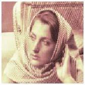
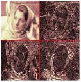
463 Original image Decomposition at level 1 Decomposition at level 2