repetition, part ii Ole-Johan Skrede INF Digital Image Processing

Transcription

1 repetition, part ii Ole-Johan Skrede INF Digital Image Processing Department of Informatics The Faculty of Mathematics and Natural Sciences University of Oslo

2 today s lecture Coding and compression Information theory Shannon-Fano coding Huffman coding Arithmetic coding Difference transform Run-length coding Lempel-Ziv-Welch coding Lossy JPEG compression Binary morphology Fundamentals: Structuring element, erosion and dilation Opening and closing Hit-or-miss transform Morphological thinning 1

3 coding and compression i

4 compression and decompression Figure 1: Compression and decompression pipeline We would like to compress our data, both to reduce storage and transmission load. In compression, we try to create a representation of the data which is smaller in size, while preserving vital information. That is, we throw away redundant information. The original data (or an approximated version) can be retrieved through decompression. 3

5 compression Figure 2: Three steps of compression We can group compression in to three steps: Transformation: A more compact image representation. Qunatization: Representation approximation. Coding: Transformation from one set of symbols to another. Encoding: Coding from an original format to some other format. E.g. encoding a digital image from raw numbers to JPEG. Decoding: The reverse process, coding from some format to the original. E.g. decoding a JPEG image back to raw numbers. 4

6 lossy and lossless compression Compression can either be lossless or lossy. There exists a number of methods for both types. Lossless: We are able to perfectly reconstruct the original image. Lossy: We can only reconstruct the original image to a certain degree (but not perfect). 5

7 redundancy We can use a different amount of data on the same signal. E.g. the signal 13 ISO (Latin-1): 16 bits: 8 bits for 1 (at 0x31) and 8 bits for 3 (at 0x33). 8-bit natural binary encoding: 8 bits: bit natural binary encoding: 4 bits: 1101 Redundancy: What can be removed from the data without loss of (relevant) information. In compression, we want to remove redundant bits. 6

8 different types of redundancy Psychovisual redundancy Information that we cannot percieve. Can be compressed by e.g. subsampling or by reducing the number of bits per pixel. Inter-pixel temporal redundancy Correlation between successive images in a sequence. A sequence can be compressed by only storing some frames, and then only differences for the rest of the sequence. Inter-pixel spatial redundancy Correlation between neighbouring pixels within an image. Can be compressed by e.g. run-length methods. Coding redundancy Information is not represented optimally by the symbols in the code. This is often measured as the difference between average code length and some theoretical minimum code length. 7

9 compression rate and redundancy The compression rate is defined as the ratio between the uncompressed size and compressed size Uncompressed size Compression rate = Compressed size or as the ratio between the mean number of bits per symbol in the compressed and uncompressed signal. Space saving is defined as the reduction in size relative to the uncompressed size, and is given as Compressed size Space savings = 1 Unompressed size Example: An 8-bit image has an uncompressed size of 256 kib, and a size of 64 kib after compression. Compression rate: 4 Space saving: 3/4 8

10 expected code length The expected length L c of a source code c for a random variable X with pmf. p X is defined as L c = p X (x)l c (x) x X where l c (x) is the length of the codeword assigned to x in this source code. Example: Let X be a random variable taking values in {1, 2, 3, 4} with probabilities defined by p X below. Let us encode this with a variable length source code c v, and a source code c e with equal length codewords. p X (1) = 1 2 c v (1) = 0 c e (1) = 00 p X (2) = 1 4 c v (2) = 10 c e (2) = 01 p X (3) = 1 8 c v (3) = 110 c e (3) = 10 p X (4) = 1 8 c v (4) = 111 c e (4) = 11 Expected length of the variable length coding: L cv = 1.75 bits. Expected length of the equal length coding: L ce = 2 bits. 9

11 information content We use information content (aka self-information or surprisal) to measure the level of information in an event X. The information content I X (x) (measured in bits) of an event x is defined as It can also be measured in nats I X (x) = log 2 1 p X (x). I X (x) = log e 1 p X (x), that is, with the natural logarithm, or in hartleys I X (x) = log 10 1 p X (x). If an event X takes value x with probability 1, the information content I X (x) = 0. 10

12 entropy The entropy of a random variable X taking values x X, and with pmf. p X, is defined as H(X) = p X (x)i X (x) x X = p X (x) log p X (x), x X and is thus the expected information content in X, measured in bits (unless another base for the logarithm is explicitly stated). We use the convention that x log(x) = 0 when x = 0. The entropy of a signal (a collection of events) gives a lower bound on how compact the sequence can be encoded (if every event is encoded separately). The entropy of a fair coin toss is 1 bit (since log = 1) The entropy of a fair dice toss is 2.6 bit (since log ) 11

13 estimating the probability mass function We can estimate the probability mass function with the normalized histogram. For a signal of length n with symbols taking values in the alphabeth {s 0,..., s m 1 }, let n i be the number of occurances of s i in the signal, then the normalized histogram value for symbol s i is p i = n i n. If one assume that the values in the signal are independent realizations of an underlying random variable, then p i is an estimate on the probability that the variable is s i. 12

14 shannon-fano coding A simple method that produces an instantaneous code. The resulting is quite compact (but not optimal). Algorithm that produces a binary Shannon-Fano code (with alphabeth {0, 1}): 1. Sort the symbols x i of the signal that we want to code by probability of occurance. 2. Split the symbols into two parts with approximately equal accumulated probability. One group is assigned the symbol 0, and the other the symbol 1. Do this step recursively (that is, do this step on every subgroup), until the group only contain one element. 3. The result is a binary tree with the symbols that are to be encoded in the leaf nodes. 4. Traverse the tree from root to the leaf nodes and record the sequence of symbols in order to produce the corresponding codeword. 13

15 shannon-fano example Two different encodings of the sequence HALLO. x p X (x) c(x) l(x) L 2/5 0 1 H 1/ A 1/ O 1/ c(hallo) = , with length 10 bits. x p X (x) c(x) l(x) L 2/ H 1/ A 1/ O 1/ c(hallo) = , with length 10 bits. 14

16 huffman coding An instantaneous coding algorithm. Optimal in the sense that it achieves minimal coding redundancy. Algorithm for encoding a sequence of n symbols with a binary Huffman code and alphabeth {0, 1}: 1. Sort the symbols by decreasing probability. 2. Merge the two least likely symbols to a group and give the group a probability equal to the sum of the probabilities of the members in the group. Sort the new sequence by decreasing probability. 3. Repeat step 2. until there are only two groups left. 4. Represent the merging as a binary tree, and assign 0 to the left branch and 1 to the right branch. 5. Every symbol in the original sequence is now at a leaf node. Traverse the tree from the root to the corresponding leaf node, and append the symbols from the traversal to create the codeword. 15

17 huffman coding: example The six most common letters in the english language, and their relative occurance frequency (normslized within this selection), is given in the table below. The resulting Huffman source code is given as c. x p(x) c(x) a e i n o t Figure 3: Huffman procedure example with resulting binary tree. 16

18 huffman coding: example The expected codeword length in the previous example is L = i l i p i = = And the entropy is H = i p i log 2 p i Thus, the coding redundancy is L H

19 ideal and actual code-word length For an optimal code, the expected codeword length L must be equal to the entropy p(x)l(x) = p(x) log 2 p(x) x x That is, l(x) = log 2 (1/p(x)), which is the information content of the event x. Figure 4: Ideal and actual codeword length from example in fig. 3 18

20 when does huffman coding not give any coding redundancy The ideal codeword length is l(x) = log 2 (1/p(x)) Since we only deal with integer codeword lengths, this is only possible when for some integer k. Example p(x) = 1 2 k x x 1 x 2 x 3 x 4 x 5 x p(x) c(x) In this example L = H = , that is, no coding redundancy. 19

21 arithmetic coding Lossless compression method. Variable code length, codes more probable symbols more compactly. Contrary to Shannon-Fano coding and Huffman coding, which codes symbol by symbol, arithmetic coding encodes the entire signal to one number d [0, 1). Same expected codeword length as Huffman code. Can achieve shorter codewords for the entire sequence than Huffman code. This is because one is not limited to integer codewords for each symbol. 20

22 arithmetic coding: encoding overview The signal is a string of symbols x, where the symbols are taken from some alphabeth X. As usual, we model the symbols as realizations of a discrete random variable X with an associated probability mass function p X. For each symbol in the signal, we use the pmf. to associate a unique interval with the part of the signal we have processed so far. At the end, when the whole signal is processed, we are left with a decimal interval which is unique to the string of symbols that is our signal. We then find the number within this decimal with the shortest binary representation, and use this as the encoded signal. 21

23 arithmetic encoding: example Suppose we have an alphabeth {a 1, a 2, a 3, a 4 } with associated pmf. p X = [0.2, 0.2, 0.4, 0.2]. We want to encode the sequence a 1 a 2 a 3 a 3 a 4. Step-by-step solution, current interval is initialized to [0, 1). Symbol Interval Sequence Interval a 1 [0.0, 0.2) a 1 [0.0, 0.2) a 2 [0.2, 0.4) a 1 a 2 [0.04, 0.08) a 3 [0.4, 0.8) a 1 a 2 a 3 [0.056, 0.072) a 3 [0.4, 0.8) a 1 a 2 a 3 a 3 [0.0624, ) a 4 [0.8, 1.0) a 1 a 2 a 3 a 3 a 4 [ , ) 22

24 arithmetic decoding Given an encoded signal b 1 b 2 b 3 b k, we first find the decimal representation d = k ( 1 b n 2 n=1 Similar to what we did in the encoding, we define a list of interval edges based on the pmf q = [0, p X (x 1 ), p X (x 1 ) + p X (x 2 ),..., k i=1 p X(x k ),...] 1. See what interval the decimal number lies in, set this as the current interval. 2. Decode the symbol corresponding to this interval (this is found via the alphabeth and q). 3. Scale the q to lie within the current interval. 4. Do step 1 to 3 until termination. Termination: Define a eod symbol (end of data), and stop when this is decoded. Note that this will also need an associated probability in the model. Or, only decode a predefined number of symbols. ) n 23

25 decoding: example Alphabeth: {a, b, c}. p X = [0.6, 0.2, 0.2]. q = [0.0, 0.6, 0.8, 1.0] Signal to decode: First, we find that = Then we continue decoding symbol for symbol until termination: [c min, c max ) q new Symbol Sequence [0.0, 1.0) [0.0, 0.6, 0.8, 1.0) a a [0.0, 0.6) [0.0, 0.36, 0.48, 0.6) c ac [0.48, 0.6) [0.48, 0.552, 0.576, 0.6) a aca [0.48, 0.552) [0.48, , , 0.552) b acab [0.5232, ) [0.5232, , , ) a acaba 24

26 coding and compression ii

27 difference transform Horizontal pixels have often quite similar intensity values. Transform each pixelvalue f(x, y) as the difference between the pixel at (x, y) and (x, y 1). That is, for an m n image f, let g[x, 0] = f[x, 0], and g[x, y] = f[x, y] f[x, y 1], y {1, 2,..., n 1} (1) for all rows x {0, 1,..., m 1}. Note that for an image f taking values in [0, 2 b 1], values of the transformed image g take values in [ (2 b 1), 2 b 1]. This means that we need to use b + 1 bits for each g(x, y) if we are going to use equal-size codeword for every value. Often, the differences are close to 0, which means that natural binary coding of the differences are not optimal. (a) Original (b) Graylevel intensity histogram Figure 5: H 7.45 = cr 1.1 (a) Difference transformed (b) Graylevel intensity histogram Figure 6: H 5.07 = cr

28 run-length transform Often, images contain objects with similar intensity values. Run-length transform use neighbouring pixels with the same value. Note: This requires equality, not only similarity. Run-length transform is compressing more with decreasing complexity. The run-length transform is reversible. Codes sequences of values into sequences of tuples: (value, run-length). Example: Values (24 numbers): 3, 3, 3, 3, 3, 3, 5, 5, 5, 5, 5, 5, 5, 5, 5, 5, 4, 4, 7, 7, 7, 7, 7, 7. Code (8 numbers): (3, 6), (5, 10), (4, 2), (7, 6). The coding determines how many bits we use to store the tuples. 27

29 run-length transform in binary images In a binary image, we can ommit the value in coding. As long as we know what value is coded first, the rest have to be alternating values. 0, 0, 0, 0, 0, 1, 1, 1, 1, 1, 1, 0, 0, 1, 1, 1, 0, 0, 0, 0, 0, 1, 1, 1, 1 5, 6, 2, 3, 5, 4 The histogram of the run-lengths is often not flat, entropy-coding should therefore be used to code the run-length sequence. 28

30 lempel-ziv-welch coding A member of the LZ* family of compression schemes. Utilizes patterns in the message by looking at symbol occurances, and therefore mostly reduces inter sample redundancy. Maps one symbol sequence to one code. Based on a dictionary between symbol sequence and code that is built on the fly. This is done both in encoding and decoding. The dictionary is not stored or transmitted. The dictionary is initialized with an alphabeth of symbols of length one. 29

31 lzw encoding example Message: ababcbababaaaaabab# Initial dictionary: { #:0, a:1, b:2, c:3 } New dictionary entry: current string plus next unseen symbol Current New dict Message string Codeword entry ababcbababaaaaabab# a 1 ab:4 ababcbababaaaaabab# b 2 ba:5 ababcbababaaaaabab# ab 4 abc:6 ababcbababaaaaabab# c 3 cb:7 ababcbababaaaaabab# ba 5 bab:8 ababcbababaaaaabab# bab 8 baba:9 ababcbababaaaaabab# a 1 aa:10 ababcbababaaaaabab# aa 10 aaa:11 ababcbababaaaaabab# aa 10 aab:12 ababcbababaaaaabab# bab 8 bab#:13 ababcbababaaaaabab# # 0 Encoded message: 1,2,4,3,5,8,1,10,10,8,0. Assuming original bps = 8, and coded bps = 4, we achieve a compression rate of c r = (2)

32 lzw decoding example Encoded message: 1,2,4,3,5,8,1,10,10,8,0 Initial dictionary: { #:0, a:1, b:2, c:3 } New dictionary entry: current string plus first symbol in next string Current New dict entry Message string Final Proposal 1,2,4,3,5,8,1,10,10,8,0 a a?:4 1,2,4,3,5,8,1,10,10,8,0 b ab:4 b?:5 1,2,4,3,5,8,1,10,10,8,0 ab ba:5 ab?:6 1,2,4,3,5,8,1,10,10,8,0 c abc:6 c?:7 1,2,4,3,5,8,1,10,10,8,0 ba cb:7 ba?:8 1,2,4,3,5,8,1,10,10,8,0 bab bab:8 bab?:9 1,2,4,3,5,8,1,10,10,8,0 a baba:9 a?:10 1,2,4,3,5,8,1,10,10,8,0 aa aa:10 aa?:11 1,2,4,3,5,8,1,10,10,8,0 aa aaa:11 aa?:12 1,2,4,3,5,8,1,10,10,8,0 bab aab:12 bab?:13 1,2,4,3,5,8,1,10,10,8,0 # bab#:13 Decoded message: ababcbababaaaaaabab# 31

33 lzw compression, summary The LZW codes are normally coded with a natural binary coding. Typical text files are usually compressed with a factor of about 2. LZW coding is used a lot In the Unix utility compress from In the GIF image format. An option in the TIFF and PDF format. Experienced a lot of negative attention because of (now expired) patents. The PNG format was created in 1995 to get around this. The LZW can be coded further (e.g. with Huffman codes). Not all created codewords are used. We can limit the number of generated codewords. Setting a limit on the number of codewords, and deleting old or seldomly used codewords. Both the encoder and decoder need to have the same rules for deleting. 32

34 lossy jpeg compression: start Each image channel is partitioned into blocks of 8 8 piksels, and each block can be coded separately. For an image with 2 b intensity values, subtract 2 b 1 to center the image values around 0 (if the image is originally in an unsigned format). Each block undergoes a 2D DCT. With this, most of the information in the 64 pixels is located in a small area in the Fourier space. Figure 7: Example block, subtraction by 128, and 2D DCT. 33

35 lossy jpeg compression: loss of information Each of the frequency-domain blocks are then point-divided by a quantization matrix. The result is rounded off to the nearest integer. his is where we lose information, but also why we are able to achieve high compression rates. This result is compressed by a coding method, before it is stored or transmitted. The DC and AC components are treated differently. Figure 8: Divide the DCT block (left) with the quantization matrix (middle) and round to nearest integer (right) 34

36 lossy jpeg compression: ac-components (sequential modes) 1. The AC-components are zig-zag scanned: The elements are ordered in a 1D sequence. The absolute value of the elements will mostly descend through the sequence. Many of the elements are zero, especially at the end of the sequence. 2. A zero-based run-length transform is performed on the sequence. 3. The run-length tuples are coded by Huffman or arithmetic coding. The run-length tuple is here (number of 0 s, number of bits in non-0 ). Arithmetic coding often gives 5 10% better compression. Figure 9: Zig-zag gathering of AC-components into a sequence. 35

37 lossy jpeg compression: dc-component 1. The DC-components are gathered from all the blocks in all the image channels. 2. These are correlated, and are therefore difference-transformed. 3. The differences are coded by Huffman coding or arithmetic coding. More precise: The number of bits in each difference is entropy coded. 36

38 lossy jpeg decompression: reconstruction of frequency-domain blocks The coding part (Huffman- and arithmetic coding) is reversible, and gives the AC run-length tuples and the DC differences. The run-length transform and the difference transform are also reversible, and gives the scaled and quantized 2D DCT coefficients The zig-zag transform is also reversible, and gives (together with the restored DC component) an integer matrix. This matrix is multiplied with the quantization matrix in order to restore the sparse frequency-domain block. Figure 10: Multiply the quantized DCT components (left) with the quantization matrix (middle) to produce the sparse frequency-domain block (right). 37

39 lossy jpeg decompression: quality of restored dct image Figure 11: Comparison of the original 2D DCT components (left) and the restored (right) The restored DCT image is not equal to the original. But the major features are preserved Numbers with large absolute value in the top left corner. The components that was near zero in the original, are exactly zero in the restored version. 38

40 lossy jpeg decompression: inverse 2d dct We do an inverse 2D DCT on the sparse DCT component matrix. f(x, y) = 2 m n ( ) ( (2x + 1)uπ (2y + 1)vπ c(u)c(v)f (u, v) cos cos mn 2m 2n where u=0 v=0 1 c(a) = 2 if a = 0, 1 otherwise. ), (3) We have then a restored image block which should be approximately equal to the original image block. (4) Figure 12: A 2D inverse DCT on the sparse DCT component matrix (left) produces an approximate image block (right) 39

41 lossy jpeg decompression: approximation error Figure 13: The difference (right) between the original block (left) and the result from the JPEG compression and decompression (middle). The differences between the original block and the restored are small. But they are, however, not zero. The error is different on neighbouring pixels. This is especially true if the neighbouring pixels belong to different blocks. The JPEG compression/decompression can therefore introduce block artifacts, which are block patterns in the reconstructed image (due to these different errors). 40

42 block artifacts and compression rate (a) Compressed (b) Difference (c) Detail (d) Compressed (e) Difference (f) Detail Figure 14: Top row: compression rate = Bottom row: compression rate =

43 morphology on binary images

44 binary images as sets Let f : Ω {0, 1} be an image. In the case of a 2D image, Ω Z 2, and every pixel (x, y) in f is in the set Ω, written (x, y) Ω. A binary image can be described by the set of foreground pixels, which is a subset of Ω. Therefore, we might use notation and terms from set theory when describing binary images, and operations acting on them. The complement of a binary image f is h(x, y) = f c (x, y) { 0 if f(x, y) = 1, = 1 if f(x, y) = 0. (a) Contours of sets A and B inside a set U (b) The complement A c (gray) of A (white) Figure 15: Set illustrations, gray is foreground, white is background. 43

45 binary images as sets The union of two binary images f and g is h(x, y) = (f g)(x, y) = { 1 if f(x, y) = 1 or g(x, y) = 1, 0 otherwise. (a) Union of A and B The intersection of two binary images f and g is h(x, y) = (f g)(x, y) = { 1 if f(x, y) = 1 and g(x, y) = 1, 0 otherwise. (b) Intersection of A and B Figure 16: Set illustrations, gray is foreground, white is background. 44

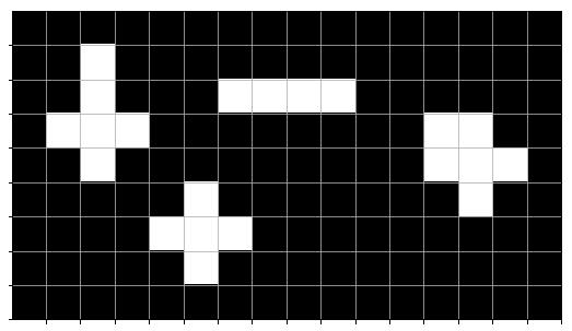
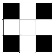
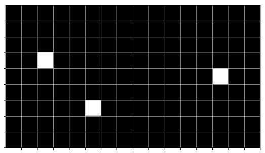
46 structuring element A structuring element in morphology is used to determine the acting range of the operations. It is typically defined as a binary matrix where pixels valued 0 are not acting, and pixels valued 1 are acting. When hovering the structuring element over an image, we have three possible scenario for the structuring element (or really the location of the 1 s in the structuring element): It is not overlapping the image foreground (a miss). It is partly overlapping the image foreground (a hit). It is fully overlapping the image foreground (it fits). Figure 17: A structuring element (top left) and a binary image (top right). Bottom: the red misses, the blue hits, and the green fits. 45

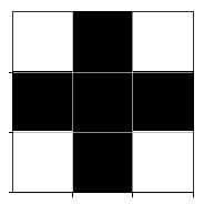
47 origin of structuring element Figure 18: Some structuring elements. The red pixel contour highlights the origin. The structuring element can have different shapes and sizes. We need to determine an origin. This origin denotes the pixel that (possibly) changes value in the result image. The origin may lay outside the structuring element. The origin should be highlighted, e.g. with a drawed square. We will assume the origin to be at the center pixel of the structuring element, and not specify the location unless this is the case. 46

48 erosion Let f : Ω f {0, 1} be a 2D binary image. Let s : Ω s {0, 1} be a 2D binary structuring element. Let x, y Z 2 be 2D points for notational convenience. We then have 3 equivalent definitions of erosion. The one mentioned at the beginning of the lecture (f s)(x) = min y Ω + s x+y Ω f {f(x + y)}, (5) where Ω + s is the subset of Ω s with foreground pixels. Place the s such that its origin overlaps with x, then 1 if s fits in f, (f s)(x) = 0 otherwise. (6) Let F (g) be the set of all foreground pixels of a binary image g, then F (f s) = {x Ω f : F (x + Ω + s ) F (f)}. (7) Note that the F () is often ommitted, as we often use set operations in binary morphology. 47

49 erosion examples (a) f (b) s 1 (c) f s 1 (a) f (b) s 2 (c) f s 2 48

50 edge detection with erosion Erosion removes pixels along the boundary of the foreground object. We can locate the edges by subtracting the eroded image from the original g = f (f s) The shape of the structuring element determines the connectivety of the countour. That is, if the contour is connected using a 4 or 8 connected neighbourhood. 49

51 edge detection with erosion: examples (a) f (b) s (c) f (f s) 50

52 edge detection with erosion: examples (a) f (b) s (c) f (f s) 51

53 dilation Let f : Ω f {0, 1} be a 2D binary image. Let s : Ω s {0, 1} be a 2D binary structuring element. Let x, y Z 2 be 2D points for notational convenience. We then have 3 equivalent definitions of dilation. The one mentioned at the beginning of the lecture (f s)(x) = max y Ω + s x y Ω f {f(x y)}, (8) where Ω + s is the subset of Ω s with foreground pixels. Place the s such that its origin overlaps with x, then 1 if s hits f, (f s)(x) = 0 otherwise. (9) where s is s rotated 180 degrees. Let F (g) be the set of all foreground pixels of a binary image g, then F (f s) = {x Ω f : F (x + Ω + s ) F (f) } (10) 52

54 dilation examples (a) f (b) s 1 (c) f s 1 (a) f (b) s 2 (c) f s 2 53

55 edge detection with dilation Dilation adds pixels along the boundary of the foreground object. We can locate the edges by subtracting the original image from the dilated image g = (f s) f The shape of the structuring element determines the connectivety of the countour. That is, if the contour is connected using a 4 or 8 connected neighbourhood. 54

56 edge detection with dilation: examples (a) f (b) s (c) (f s) f 55

57 edge detection with dilation: examples (a) f (b) s (c) (f s) f 56

58 duality between dilation and erosion Dilation and erosion are dual operations w.r.t. complements and reflections (180 degree rotation). That is, erosion and dilation can be expressed as f s = (f c s) c f s = (f c s) c This means that dilation and erosion can be performed by the same procedure, given that we can rotate the structuring element and find the complement of the binary image. (a) f (b) s (c) f s (a) f c (b) s (c) f c s 57

59 morphological opening Erosion of an image removes all regions that cannot fit the structuring element, and shrinks all other regions. We can then dilate the result of the erosion, with this the regions that where shrinked are (approximately) restored. the regions too small to survive an erosion, are not restored. This is morphological opening f s = (f s) s The name stems from that this operation can provide an opening (a space) between regions that are connected through thin bridges, almost without affecting the original shape of the larger regions. Using erosion only will also open these bridges, but the shape of the larger regions is also altered. The size and shape of the structuring element is vital. 58

60 example: opening (a) f (b) s (c) f s Figure 29: Morphological opening of f with s. 59

61 morphological closing Dilation of an image expands foreground regions and fills small (relative to the structuring element) holes in the foreground. We can then erode the result of the dilation, then the regions that where expanded are (approximately) restored. the holes that where filled, are not opened again. This is morphological closing f s = (f s) s The name stems from that this operation can close small gaps between foreground regions, without altering the larger foreground shapes too much. Using dilation only will also close these gaps, but the shape of the larger regions is also altered. The size and shape of the structuring element is vital. 60

62 example: closing (a) f (b) s (c) f s Figure 30: Morphological opening of f with s. 61

63 duality Opening and closing are dual operations w.r.t. complements and rotation f s = (f c s) c f s = (f c s) c This means that closing can be performed by complementing the image, opening the complement by the rotated structuring element, and complement the result. The corresponding is true for opening. (a) f (b) s (c) f s (a) f c (b) s (c) f c s 62

64 hit-or-miss transformation Let f be a binary image as usual, but define s to be a tuple of two structuring elements s = (s hit, s miss ). The hit-or-miss transformation is then defined as f s = (f s hit ) (f c s miss ), A foreground pixel in the out-image is only achieved if s hit fits the foreground around the pixel, and s miss fits the background around the pixel. This can be used in several applications, including finding certain patterns in an image, removing single pixels, thinning and thickening foreground regions. 63

65 hit-or-miss example (a) f (b) s hit (c) f s hit (a) f c (b) s miss (c) f c s miss Figure 35: f s 64

66 morphological thinning Morphological thinning of an image f with a structuring element tuple s, is defined as f s = f \ (f s) = f (f s) c In order to thin a foreground region, we perform a sequential thinning with multiple structuring elements s 1,..., s 8, which, when defined with the hit-or-miss notation above are s hit 1 = s hit 2 = , s miss 1 = , s miss 2 = Following this pattern, where s i+1 is rotated clockwise w.r.t. s i, we continue this until s hit 8 = , s miss 8 =

67 morphological thinning With these previously defined structuring elements, we apply the iteration d 0 = f d k = d k 1 {s 1,, s 8 } = ( ((d k 1 s 1 ) s 2 ) ) s 8 for K iterations until d K = d K 1 and we terminate with d K as the result of the thinning. In the same manner, we define the dual operator thickening f s = f (f s), which also can be used in a sequential manner analogous to thinning. 66

68 thinning example (a) d 0 = f (b) d 01 = d 0 \ (d 0 s 1) (c) d 02 = d 01 \ (d 01 s 2) (d) d 03 = d 02 \ (d 02 s 3) (e) d 04 = d 03 \ (d 03 s 4) (f) d 05 = d 04 \ (d 04 s 5) (g) d 06 = d 05 \ (d 05 s 6) (h) d 07 = d 06 \ (d 06 s 7) (i) d 08 = d 07 \ (d 07 s 8) 67

69 thinning example (a) d 1 = d 0 (b) d 11 = d 1 \ (d 1 s 1 ) (c) d 12 = d 11 \ (d 11 s 2 ) (d) d 13 = d 12 \ (d 12 s 3 ) (e) d 14 = d 13 \ (d 13 s 4 ) (f) d 15 = d 14 \ (d 14 s 5 ) (g) d 16 = d 15 \ (d 15 s 6 ) (h) d 17 = d 16 \ (d 16 s 7 ) (i) d 18 = d 17 \ (d 17 s 8 ) 68

70 thinning example (a) d 2 = d 1 (b) d 21 = d 2 \ (d 2 s 1 ) (c) d 22 = d 21 \ (d 21 s 2 ) (d) d 23 = d 22 \ (d 22 s 3 ) (e) d 24 = d 23 \ (d 23 s 4 ) (f) d 25 = d 24 \ (d 24 s 5 ) (g) d 26 = d 25 \ (d 25 s 6 ) (h) d 27 = d 26 \ (d 26 s 7 ) (i) d 28 = d 27 \ (d 27 s 8 ) 69

71 summary Coding and compression Information theory Shannon-Fano coding Huffman coding Arithmetic coding Difference transform Run-length coding Lempel-Ziv-Welch coding Lossy JPEG compression Binary morphology Fundamentals: Structuring element, erosion and dilation Opening and closing Hit-or-miss transform Morphological thinning 70

72 Questions? 71