Logistic & Tobit Regression

Transcription

1 Logistic & Tobit Regression

2 Different Types of Regression

3 Binary Regression (D)

4

5

6

7

8 Logistic transformation + e P( y x) = 1 + e! " x! + " x " P( y x) % ln$ ' = ( + ) x # 1! P( y x) & logit of P(y x){

9 P(y x)

10

11 Log likelihood!!! = = = + " = + + " = " " + = N i w x i i N i w x i i i N i i i i i i i e w x y e w x p w x p y w x p y w x p y w l ) log(1 ) 1 1 log( ) ; ( (1 ) ; ( log )) ; ( )log(1 (1 ) ; ( log ) (

12 Log likelihood!!! = = = + " = + + " = " " + = N i w x i i N i w x i i i N i i i i i i i e w x y e w x p w x p y w x p y w x p y w l ) log(1 ) 1 1 log( ) ; ( (1 ) ; ( log )) ; ( )log(1 (1 ) ; ( log ) ( Note: this likelihood is a concave

13 Maximum likelihood estimation # # w Common (but not only) approaches: Numerical Solutions: Line Search Simulated Annealing Gradient Descent Newton s Method j l( w) = = K = # # w! j N i= 1! x ij N i= 1 ( y { y x w " log(1 + e i i " i p( x, w)) i prediction error x w i )} No closed form solution!

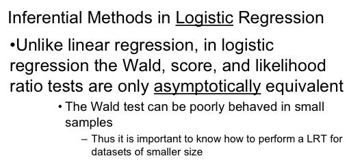
14 Statistical Inference in Logistic Regression

15

16

17 likelihood score test LRT Wald * β 0 * mle β

18 Measuring the Performance of a Binary Classifier

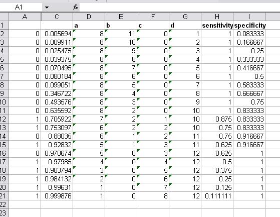
19 Training Data for a Logistic Regression Model

20 predicted probabilities Suppose we use a cutoff of 0.5 actual outcome 1 0 predicted outcome Test Data 0 0 9

21 More generally actual outcome misclassification rate: b + c a+b+c+d 1 0 predicted outcome 1 0 a c b d sensitivity: specificity: (aka recall) predicitive value positive: a a+c d b+d a a+b (aka precision)

22 Suppose we use a cutoff of 0.5 actual outcome predicted outcome sensitivity: = 100% 8+0 specificity: = 75% 9 9+3

23 Suppose we use a cutoff of 0.8 actual outcome predicted outcome sensitivity: = 75% 6+2 specificity: = 83%

24 Note there are 20 possible thresholds ROC computes sensitivity and specificity for all possible thresholds and plots them Note if threshold = minimum c=d=0 so sens=1; spec=0 If threshold = maximum a=b=0 so sens=0; spec=1 1 0 actual outcome 1 0 a b c d

25

26

27 Area under the curve is a common measure of predictive performance So is squared error: Σ(y i -yhat) 2 also known as the Brier Score

28 Penalized Logistic Regression

29 Ridge Logistic Regression Maximum likelihood plus a constraint: p! j= 1 # 2 j " s Lasso Logistic Regression Maximum likelihood plus a constraint: p! j= 1 # j " s

30 s

31

32

33 Polytomous Logistic Regression (PLR) P( y i = k x i ) = exp( r! k x i ) exp( r! k ' x i ) " k ' Elegant approach to multiclass problems Also known as polychotomous LR, multinomial LR, and, ambiguously, multiple LR and multivariate LR

34 1-of-K Sample Results: brittany-l POS 1suff 1suff*POS 2suff 2suff*POS 3suff 3suff*POS 3suff+POS+3suff*POS+Arga mon All words Feature Set Argamon function words, raw tf % errors Number of Features authors with at least 50 postings. 10,076 training documents, 3,322 test documents. BMR-Laplace classification, default hyperparameter 4.6 million parameters

35 Generalized Linear Model Adrian Dobra

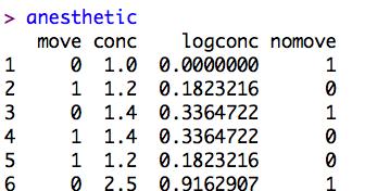
36 Logistic Regression in R plot(nomove~conc,data=anesthetic)

37

38

39 > anes.logit <- glm(nomove ~ conc, family=binomial(link="logit"), data=anesthetic) > summary(anes.logit) Call: glm(formula = nomove ~ conc, family = binomial(link = "logit"), data = anesthetic) Deviance Residuals: Min 1Q Median 3Q Max Coefficients: Estimate Std. Error z value Pr(> z ) (Intercept) ** conc ** --- Signif. codes: 0 *** ** 0.01 * (Dispersion parameter for binomial family taken to be 1) Null deviance: on 29 degrees of freedom Residual deviance: on 28 degrees of freedom AIC: Number of Fisher Scoring iterations: 5

40 Deviance Residuals: r D (i) = sign(y i " ˆ y i ) D(y i,#)

41

42 data(frogs) plot(northing ~ easting, data=frogs, pch=c(1,16)[frogs$pres.abs+1], xlab="meters east of reference point", ylab="meters north")

43

44 > frogs.glm0 <- glm(pres.abs ~.,data=frogs,family=binomial(link=logit)) > summary(frogs.glm0) Call: glm(formula = pres.abs ~., family = binomial(link = logit), data = frogs) Deviance Residuals: Min 1Q Median 3Q Max Coefficients: Estimate Std. Error z value Pr(> z ) (Intercept) e e northing 1.041e e easting e e altitude 7.091e e distance e e * NoOfPools 2.968e e ** NoOfSites 4.294e e avrain e e meanmin 1.564e e * meanmax 1.708e e Null deviance: on 211 degrees of freedom Residual deviance: on 202 degrees of freedom AIC:

45 > frogs.glm1 <- glm(pres.abs ~ easting + distance + NoOfPools + meanmin,data=frogs,family=binomial(link=logit)) > summary(frogs.glm1) Call: glm(formula = pres.abs ~ easting + distance + NoOfPools + meanmin, family = binomial(link = logit), data = frogs) Deviance Residuals: Min 1Q Median 3Q Max Coefficients: Estimate Std. Error z value Pr(> z ) (Intercept) * easting distance *** NoOfPools ** meanmin ** Null deviance: on 211 degrees of freedom Residual deviance: on 207 degrees of freedom AIC: AIC not as good

46 > CVbinary(frogs.glm0) Fold: Internal estimate of accuracy = Cross-validation estimate of accuracy = > CVbinary(frogs.glm1) Fold: Internal estimate of accuracy = Cross-validation estimate of accuracy = CV accuracy estimates quite variable with small datasets Best to repeat comparing models on same split

47 all.acc <- numeric(10) red.acc <- numeric(10) for (j in 1:10) { randsam <- sample (1:10,dim(frogs)[1], replace=true) all.acc[j] <- CVbinary(frogs.glm0, rand=randsam)$acc.cv red.acc[j] <- CVbinary(frogs.glm1, rand=randsam)$acc.cv } > all.acc [1] > red.acc [1]

48 par(mfrow=c(3,3)) for (i in 2:10) { } ints <- pretty(frogs[,i],n=10) J <- length(ints)-2 y <- n <- x <- rep(0,j-1) for (j in 2:J) { } temp <- frogs[((frogs[,i]>ints[j]) & (frogs[,i]<=ints[j+1])),]; y[j-1] <- sum(temp$pres.abs); n[j-1] <- dim(temp)[1]; x[j-1] <- (ints[j]+ints[j+1])/2; y <- logit((y+0.5)/(n+1)) # plot(x,y,type="b",col="red") # par(new=true) plot(lowess(x,y), main=names(frogs)[i], type="l", col="red")

49

50 > frogs.glm2 <- glm(pres.abs ~ northing + easting + altitude + distance + I(distance^2)+ NoOfPools + NoOfSites + avrain + meanmin + meanmax, data=frogs,family=binomial(link=logit)) Estimate Std. Error z value Pr(> z ) (Intercept) e e northing 4.852e e easting e e altitude 8.864e e distance e e ** I(distance^2) 4.270e e NoOfPools 2.992e e ** NoOfSites 7.765e e avrain e e meanmin 1.618e e * meanmax 2.966e e Signif. codes: 0 *** ** 0.01 * (Dispersion parameter for binomial family taken to be 1) Null deviance: on 211 degrees of freedom Residual deviance: on 201 degrees of freedom AIC:

51 glm(formula = pres.abs ~ northing + easting + altitude + log(distance) + NoOfPools + NoOfSites + avrain + meanmin + meanmax, family = binomial(link = logit), data = frogs) Deviance Residuals: Min 1Q Median 3Q Max Coefficients: Estimate Std. Error z value Pr(> z ) (Intercept) e e northing 9.661e e easting e e altitude 6.550e e log(distance) e e ** NoOfPools 2.813e e ** NoOfSites 1.897e e avrain e e meanmin 1.463e e * meanmax 1.336e e Signif. codes: 0 *** ** 0.01 * (Dispersion parameter for binomial family taken to be 1) Null deviance: on 211 degrees of freedom Residual deviance: on 202 degrees of freedom AIC: CVbinary:

52 Other things to try changepoints more log, ^2, exp, etc. > frogs.glm3 <- glm(pres.abs ~ northing + easting + altitude+ log(distance)+ NoOfPools + NoOfSites + avrain + log(meanmin) + meanmax + I(avrain*(avrain>155)),data=frogs,family=binomial(link=logit))

53 Latent Variable Interpretations Suppose our binary dependent variable depends on an unobserved utility index, Y * If Y is discrete taking on the values 0 or 1 if someone buys a car, for instance Can imagine a continuous variable Y * that reflects a person s desire to buy the car Y * would vary continuously with some explanatory variable like income

54 Logit and Probit Models Written formally as If the utility index is high enough, a person will buy a car If the utility index is not high enough, a person will not buy a car

55 Logit and Probit Models The basic problem is selecting F the cumulative density function for the error term This is where where the two models differ

56 Logit Model For the logit model we specify Prob(Y i = 1) 0 as β 0 + β 1 X 1i Prob(Y i = 1) 1 as β 0 + β 1 X 1i Thus, probabilities from the logit model will be between 0 and 1

57 Probit Model In the probit model, we assume the error in the utility index model is normally distributed ε i ~ N(0,σ 2 ) Where F is the standard normal cumulative density function (c.d.f.)

58 The Tobit Model Can also have latent variable models that don t involve binary dependent variables Say y* = xβ + u, u x ~ Normal(0,σ 2 ) But we only observe y = max(0, y*) The Tobit model uses MLE to estimate both β and σ for this model Important to realize that β estimates the effect of x on y*, the latent variable, not y

59 Conceptualizing Censored Data What do we make of a variable like Hersheys chocolate bars consumed in the past year? For all the respondents with 0 bars, we think of those cases as left censored from below. Think of a latent variable for willingness to consume Hershey bars that underlies bars consumed in the past year. Individuals who most detest Hershey Bars would score a negative number of bars consumed if that were possible.

60 Censored Regression Models & Truncated Regression Models More general latent variable models can also be estimated, say y = x β + u, u x,c ~ Normal(0, σ 2 ), but we only observe w = min(y,c) if right censored, or w = max(y,c) if left censored Truncated regression occurs when rather than being censored, the data is missing beyond a censoring point

61 Estimation Probability Pr[ Y = 0 X ] = Pr[ X! + " $ 0 X ] = Pr[ " $ % X! X ] i i i i i i i i &" i X i! ' ( X i! ) = Pr - $ % X i = * + %, # #. / 0 1 # 2 # X i! $ Pr[ Yi > 0 X i ] = 1% & ' % ( ) " *

62 Estimation see how OLS biased Standard Tobit with: N = 30 K = 2 #" 2 $! = % 0.5 & ' (! =1

63 Empirical Example (Extramarital Affairs) A Theory of Extramarital Affairs, Ray C.Fair, observations Left-censored at 0; Right-censored at 12 Steps: 1. Guess the signs of coefficients 2. Build the final model (compare to our guess) 3. Who are the most and least restraint?

64 Introduce Variables & Guess signs y_pt = number of extramarital affairs (annually) (0, 1, 2, 3, 7 ~ 4-10 times, 12 ~ more than 12) Z1= male dummy (+) Z2= age (-) Z3= number of years married (+) Z4= child dummy (-) Z5= How religious (-) Z6= Level of education (ambiguous) Z7= occupation (ambiguous) Z8= marriage satisfaction (-)

65 Variables OLS 601 Tobit OLS 150 Constant (0.7753) (2.6588) (1.4254) Z age (0.0216) (0.0777) Z number of years married (0.0367) (0.1342) (0.0651) Z religiousness (0.1112) (0.4047) (0.2844) Z self-rating of marriage (0.1183) (0.0408) (0.2737)

66 A weakness of the Tobit model The Tobit model makes the same assumptions about error distributions as the OLS model, but it is much more vulnerable to violations of those assumptions. In an OLS model with heteroskedastic errors, the estimated standard errors can be too small. In a Tobit model with heteroskedastic errors, the computer uses a bad estimate of the error distribution to determine the chance that a case would be censored, and the coefficient is badly biased.

67 Data set with heteroskedastic error distribution This data set still has Y = X + e, but the range of e increases with X y x

68 OLS with heteroskedastic error The OLS regression model still gives good values for the slope and intercept, but you can t really trust the t scores.. * try models with heteroskedastic error terms. generate e2 = x*zscore. generate y2 = x + e2. regress y2 x Source SS df MS Number of obs = F( 1, 98) = Model Prob > F = Residual R-squared = Adj R-squared = Total Root MSE = y2 Coef. Std. Err. t P> t [95% Conf. Interval] x _cons

69 Tobit with heteroskedastic error The Tobit model gives values for the slope and intercept that are simply incorrect. (Too steep) Tobit estimates Number of obs = 100 LR chi2(1) = Prob > chi2 = Log likelihood = Pseudo R2 = y2 Coef. Std. Err. t P> t [95% Conf. Interval] x _cons _se (Ancillary parameter) Obs. summary: 55 left-censored observations at y2<=3 45 uncensored observations

70 Summary of Tobit models Tobit models can be very useful, but you must be extremely careful. Graph the relationship between each explanatory variable and the outcome variable. Look for evidence that the errors are not identically and normally distributed.