Modelling Non-homogeneous Markov Processes via Time Transformation

Transcription

1 Modelling Non-homogeneous Markov Processes via Time Transformation Biostat 572 Jon Fintzi

2 Structure of the Talk Recap and motivation Derivation of estimation procedure Simulating data Ongoing/next steps

3 Motivation - Scientic Objectives Scientic Goal: Describe a disease process in terms of its transitions through discrete states. Progressive disease: subjects traverse disease states in one direction. Stages of HIV infection Non-progressive disease: subjects may visit some or all states repeatedly, just once, or not at all. Delirium

4 Motivation - Methodological Objectives Goal:Obtain estimates and covariance matrices for transition intensity parameters in non-homogeneous Markov process models. Problem #1 - Panel Data: Subjects are observed at a sequence of discrete times, observations consist of the states occupied by the subjects at those times. The exact transition times are not observed. The complete sequence of states visited by a subject may not be known.

5 Motivation - Methodological Objectives

6 Motivation - Methodological Objectives

7 Motivation - Methodological Objectives Problem #1 - Panel Data: Solution by Kalbeisch & Lawless Estimation of transition parameters for homogeneous Markov processes via maximum likelihood. A process is Markov if the future state of the process depends only on its current state. i.e. P (X (t + s) = j X (t) = i, X (u) = x(u), 0 u < s) = P (X (t + s) = j X (t) = i) = p ij (t, t+s) A process is homogeneous if the transition probabilities do not depend on the chronological time t. i.e. p ij (t, t + s) = p ij (s) Fisher scoring algorithm based on expectations of rst order derivatives of the log-likelihood provides parameter and variance estimates.

8 Motivation - Methodological Objectives Problem #2 -Non-homogeneity in the Markov Process If the process is non-homogeneous, p ij (t, t + s) p ij (s), so we must estimate a new transition probability matrix for every t. Contribution of this paper: If all of the non-homogeneity in the process is purely due to a time-varying multiplicative change in the transition intensities, we may use the results by Kalbeisch and Lawless with minor adjustments.

9 Key Proposition: Time Transformation Let u denote the original time scale of the observations. If there exists an invertible transformation of the time scale such that the process is homogeneous on t=h(u), with transition intensity matrix Q 0, then P(u 1, u 2 ) = P(h(u 1 ), h(u 2 )) = P(t 2 t 1 ) = exp[q 0 (t 2 t 1 )] = exp[q 0 (h(u 2 ) h(u 1 ))]

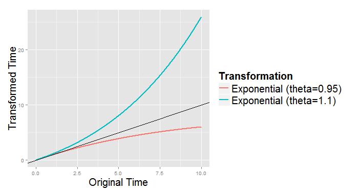
10 Key Proposition: Time Transformation Kalbeisch and Lawless suggested that nonhomogeneity arising from a transformation of the time scale could be accounted for using exp(q u2 0 u 1 g(s)ds) An advantage of the method in my paper is that it does not require that the time transformation be integrable. t = h(u) is a time scale, so we require h(u) 0 and h(u) u 0. Examples of time transformations Exponential: t = h(u; θ) = uθ u Nonparameteric: Knots at u k, k = 1,..., d t = h(u) = uθ(u) θ(u) = c(u) = d { ( )} 1 u uk c(u)θ k k=1 γ K γ d ( ) 1 u uk 1 k=1 γ K γ

11

12 Maximum Likelihood Estimation Maximum likelihood estimation for a nonhomogeneous Markov process via time transformation proceeds exactly as in Kalbeisch and Lawless. The likelihood for X = (X (u 1 ),..., X (u n )) T is: L(Q 0 ) = P(X (u 1 ) = x 1 ) n p xi 1,x i (u i 1, u i ) i=2 Since the transformed process is homogeneous, we have L(Q 0, θ) = P(X (u 1 ) = x 1 ) = P(X (u 1 ) = x 1 ) n p xi 1,x i (h(u i ; θ) h(u i 1 ; θ)) i=2 n i=2 [ e Q 0(h(u i ;θ) h(u i 1 ;θ)) ] x i 1 x i

13 Seminal Paper: Kalbeish & Lawless (1985) The scoring method proposed in Kalbeisch and Lawless, and implemented in Hubbard et al., uses the expected information matrix. This simplies the algorithm by only requiring use of the rst-order derivatives of the likelihood. Assume independence across subjects. Letting ψ be the vector of functionally independent elements of Q 0 and θ, we have that the MLEs are the solutions to ψ logl m(ψ) = 0 and ˆψ N (0, Im 1 (ψ 0 )), where I m = E [ ( ) ( ) ] T ψ logl m(ψ) ψ logl m(ψ) Given initial estimates ψ ( 0), the (k + 1) st step for the MLEs is ˆψ (k+1) = ˆψ (k) + Î m ( ˆψ (k) ) 1 ψ logl m(ψ)

14 Derivation of rst-order derivatives We require partial derivatives of P(u j 1, u j ) with respect to ψ u when ψ u is a transition intensity parameter in Q 0 and when ψ u is a parameter of the time transformation. Let A( be the matrix of eigenvectors of Q 0, and let D = e λ 1(h(u j ) h(u j 1 )),..., e λ s(h(u j ) h(u j 1 )) ), where λ 1,..., λ s are eigenvalues of Q 0. Let G u = A 1 Q 0 ψ u A, and let g (u) ij be the (i, j) entry of G u. Let h(u) = (h(u j ) h(u j 1 ))

15 Derivation of rst-order derivatives First, when ψ u Q 0, ψ u P(u j 1, u j ) = = = = ψ u e [Q 0 h(u)] Q0 s h(u) s ψ u s=1 s! Q0 s s h(u) s=1 ψ u s! s 1 s=1 l=0 s 1 = s=1 l=0 s 1 = A s=1 l=0 = AV ua 1 Q0 l Q 0 ψ u Q0 s s 1 l h(u) s! AD l A 1 Q 0 ψ u AD s 1 l A D l A 1 Q 0 ψ u AD s 1 h(u) s! s s 1 l h(u) A 1 s!

16 Derivation of rst-order derivatives where V u is an s s matrix with (i, j) element g (u) ii g (u) s 1 λ s 1 l ij i λ l h(u) s j s=1 l=0 s! s 1 [ h(uj ) h(u j 1 ) ] s=1 l=0 λ s 1 i s! [ ] [ ] = g (u) e λ i h(u j ) h(u j 1 ) e λ j h(u j ) h(u j 1 ) ij λ i λ j = g (u) [ h(uj ) h(u ii j 1 ) ] [ ] e λ i h(u j ) h(u j 1 ), i j, i = j

17 Derivation of rst-order derivatives When ψ u θ, ψ u P(u j 1, u j ) = = = e [Q 0 h(u)] ψ ( u h(uj ) ψ u ( h(uj ) ψ u h(u j 1) ψ u h(u j 1) ψ u ) Q 0 e [Q 0 h(u)] ) Q 0 P(u j 1, u j )

18 Derivation of the score function The u th element of the score function is given by l (m) u (Q0; θ) = = n m i ψ u i=1 j=2 { [ ]} log p xi,j 1 x ij h(u) m n i 1 p xi,j 1 x i=1 j=2 p xi,j 1 x ij h(u) ψ ij h(u) u

19 Derivation of the expected information matrix The (u, v) th element of the expected information matrix for one subject is given by ( ) 2 I uv (ψ) = E l(ψ) ψ uψ v n i 1 2 = E p xi,j 1 x j=2 p xi,j 1 x ij h(u) ψ ij h(u) uψ v 1 E (p xi,j 1 x ij h(u)) 2 p xi,j 1 x ψ ij h(u) p xi,j 1 x u ψ ij h(u) v

20 Derivation of the expected information matrix If we restrict ourselves to time transformation functions h(h) with second derivatives that are bounded by an integrable function, then we can exchange integration and dierentiation in the rst term in the summand. The (u, v) th element of the expected information matrix reduces to n i 1 I uv (ψ) = E j=2 (p xi,j 1 x ij h(u)) 2 p xi,j 1 x ψ ij h(u) p xi,j 1 x u ψ ij h(u) v We can estimate this by n Î uv ( ˆψ) m i 1 = E i=1 j=2 (p xi,j 1 x ij h(u)) 2 p xi,j 1 x ψ ij h(u) p xi,j 1 x u ψ ij h(u) v

21 We now have derived everything we need in order to do the estimation. Large sample properties of the estimates can be derived using standard asymptotic theory (Billingsley, 1961; Albert, 1962; Bladt and Sorensen, 2005). We can derive many other quantities from what we have shown above Asymptotic distribution of transition probabilities Mean sojourn times in each state and their variances Steady state distribution (for an ergodic process)

22 Data Simulation Procedure The o diagonal elements of Q are like the intensity parameters of independent Poisson processes from state i to state j, while diagonal elements are like the negated intensity of arrival to any non-diagonal state. We can simulate the path for homogeneous process from a given transition intensity matrix by generating transition times, then randomly selecting the new state conditional on a move. Incorporating non-homogeneity and the panel structure of observations is trivial once the path has been simulated.

23 Data Simulation Procedure We simulate data that is homogeneous on a transformed time scale as follows: 1 On the original time scale, simulate i.i.d. Unif (0.2, 1) inter-observation times. Cumulative summation gives the raw observation times. 2 Transform the observation times. This gives observation times in the operational time scale on which the process is homogeneous. 3 Simulate a path from the transition intensity matrix. Record sequence of states and transition times.

24 Data Simulation Procedure

25 Data Simulation Procedure Simulating a path proceeds as follows: 1 Given state i at time t = 0, draw u Unif (0, 1). The sojourn time in state i is given by t = log(u) q ii exp( mean = 1 q i i ) 2 Conditioned on exiting state i, the probability of moving to state j is p ij =. We then partition the interval [0, 1] q ij j i q ij into the lengths p ij for j i, and draw v Unif (0, 1). The interval into which v falls gives it's next state. 3 If the new state is an absorbing state (death), or if the transition data is greater than the termination date of the period of observation, the path is terminated. Otherwise, the state is recorded under the next time in the panel observation, we increment the time, then proceed.

26 In Progress... Currently working on debugging code. Once method is working, select implementation for competing methods. I was hopeful that I would have simulation results for this talk. Suggestions? More theory? Justication for asymptotic results? More comparison vs. other methods?