ECON 616: Lecture Two: Deterministic Trends, Nonstationary Processes

Transcription

1 ECON 616: Lecture Two: Deterministic Trends, Nonstationary Processes ED HERBST September 11, 2017

2 Background Hamilton, chapters 15-16

3 Trends vs Cycles A commond decomposition of macroeconomic time series is into trend and cycle. If Y T corresponds to real per capita GDP gdp t of the United States. According to this components approach to time series, y t is expressed as y t = ln gdp t = trend t + fluctuations t we will examine regression techniques that decompose y t in a trend and a cyclical component.

4 An identication problem what features of the time series do we regard as trend and what do we regard as uctuations around the trend? Let's guess a linear deterministic time trend: y t = β 1 + β 2 t + u t A decomposition of y t into trend and uctuations can be obtained by estimating β 1 and β 2 : y t = trend t + fluctuations t = ( ˆβ 1 + ˆβ 2 t) + (y t ˆβ 1 ˆβ 2 t). (1) When y t is logged, the coecient β 2 an average growth rate. has the interpretation of

5 Deterministic Trend Model Consider the deterministic trend model y t = β 1 + β 2 t + u t with E[u t ] = 0 and var[u t ] = σ 2. There are several diculties associated with the large sample analysis of the OLS estimators ˆβ 1,T and ˆβ 2,T. Taking x t = [1, t], 1. The matrix 1 xt x T t does not converge to a non-singular matrix Q. 2. In a time series model, the disturbances u t are in general dependent. This will change the limiting distribution of quantities such as T 1 T xt u t. 3. If the u t 's are serially correlated, then the OLS estimator will in general be inecient.

6 Rates of Convergence for OLS Estimator Roughly speaking, convergence rates tell us how fast we can learn the true value of a parameter in a sampling experiment. "standard" OLS then the variance of the ˆβ converges to zero at rate 1/T. This isn't true for models with deterministic trends. Let's look at the distributions of T ( ˆβ 0 β 0 ) and T ( ˆβ1 β 1 )

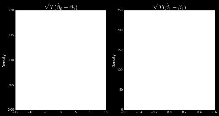
7 A Monte Carlo

8 Some math Facts: T 1 = T, t=1 T t = T (T + 1)/2, t=1 T t 2 = T (T + 1)(2T + 1)/6 t=1 (Assume u ts are independently distributed.) 1 xt x t = 1 ( 1 t T T t t 2 are not convergent! On the other hand 1 T 3 xt x t ( /3 which is singular and not invertible! Message: Trends change the rate of convergence of estimators! ) )

9 More on Rates of Convergence It turns out that ˆβ 1,T and ˆβ 2,T have dierent asymptotic rates of convergence. In particular, we will learn faster about the slope of the trend line than the intercept. To analyze the asymptotic behavior of the estimators we dene the matrix ( ) 1 0 G T =. 0 T Note that the matrix is equivalent to its transpose, that is, G T = G T.

10 Asymptotic Distributions We will analyze the following quantity G T ( ˆβ T β) = ( 1 T ) 1 ( G 1 1 T x tx tg 1 T T G 1 T x tu t ). It can be easily veried that 1 T G 1 T x tx tg 1 T = 1 T ( 1 t/t t/t (t/t ) 2 ) Q, where Q = ( 1 1/2 1/2 1/3 ).

11 Standardization The term 1 T G 1 T x tu t has the components 1 ut and T 1 T (t/t )ut which converge in probability to zero based on the weak law of large numbers for non-identically distributed random variables.. Note: Without the proper standardization 1 tut will not T converge to its expected value of zero. The variance of the random variable Tu T is getting larger and larger with sample size which prohibits the convergence of the sample mean to its expectation. Result: Suppose y t = β 1 + β 2 t + u t, u t iid(0, σ 2 ). Let ˆβ i,t, i = 1, 2 be the OLS estimators of the intercept and slope coecient, respectively. Then ˆβ 1,T β 1 p 0 (3) T ( ˆβ 2,T β 2 ) p 0. (4)

12 CLT I'm not going to show the details of proof for CLT, but We use a CLT for independently but not identically distributed random variables (Liapounov) Also, Cramer and Wold device that can be used to deduce the convergence of a random vector based on the convergence of arbitrary linear combinations of its elements. Result y t = β 1 + β 2 t + u t, u t iid(0, σ 2 ). Let ˆβ i,t, i = 1, 2 be the OLS estimators of the intercept and slope coecient, respectively. The sampling distribution of the OLS estimators has the following large sample behavior T GT ( ˆβ T β) = N (0, σ 2 Q 1 )

13 Note This is equivalent to [ ] ([ T ( ˆβ1,T β) 0 = N T 3/2 ( ˆβ 2,T β 2 ) 0 ], σ 2 [ ]).

14 Having Said All this We we consider this case where the variance is unknown: ˆσ 2 = 1 (yt T ˆβ 1 ˆβ 2 t) 2 2 Despite the fact that β 1 and β 2 have dierent asymptic rates of convergence, the t statistics still have N(0, 1) limited distribution because the standard error estimates have osetting behaviour.

15 OLS and Serial Dependence y t = βt + u t u t are serially correlated, that is, E[u t u t h ] 0 for some h = OLS not ecient. Let's look at example with MA(1) errors. can verify u t = ɛ t + θɛ t 1, ɛ t iid(0, σ 2 ɛ ). E[u 2 t ] = E[(ɛ t + θɛ t 1 ) 2 ] = (1 + θ 2 )σ 2 ɛ (5) E[u t u t 1 ] = E[(ɛ t + θɛ t 1 )(ɛ t 1 + θɛ t 2 )] = θσ 2 ɛ (6) E[u t u t h ] = 0 h > 1. (7)

16 The OLS estimator ˆβ T β = tut t 2. To nd the limiting distribution, note that 1 T 3 T t 2 = t=1 T (T + 1)(2T + 1) 6T 1 3.

17 Denominator The denominator can be manipulated as follows tut = t(ɛ t + θɛ t 1 ) = = = = 0 +ɛ 1 +2ɛ 2 +3ɛ θɛ 0 +2θɛ 1 +3θɛ 2 +4θɛ T 1 (t + θ(t + 1))ɛ t + θɛ 0 + T ɛ T t=1 T 1 T 1 (1 + θ)tɛ t + θɛ t + θɛ 0 + T ɛ T t=1 t=1 T (1 + θ)tɛ t θt ɛ T + θ t=1 T ɛ t 1 t=1 }{{} asymp. negligible. (8)

18 OLS, Continued After standardization by T 3/2 we obtain T 3/2 tut = 1 T (1 + θ) T (t/t )ɛ t 1 θɛ T + θ 1 T T T t=1 T ɛ t t=1 1. First term obeys CLT 2. Second Term goes to zero 3. Third Term goes to zero

19 Remark Consider the following model with iid disturbances y t = βt + u t, u t iid(0, σ 2 ɛ (1 + θ 2 )). The unconditional variance of the disturbances is the same as in the model with moving average disturbances. It can be veried that T 3/2 ( ˆβ T β) = ( 0, 3σ 2 ɛ (1 + θ 2 ) ). If θ is positive then the limit variance of the OLS estimator in the model with iid disturbances is smaller than in the trend model with moving average disturbances. Positive serial correlated data are less informative than iid data.

20 Stochastic Trends We looked at stationary model and deterministic trend models so far. Now we will examine univariate models with a stochastic trend of the form y t = φ 0 + y t 1 + ɛ t ɛ t iid(0, σ 2 ) This particular model is called a random walk with drift. The variable y t is said to be integrated of order one.

21 Cointegration Moreover, we will consider bivariate models with a common stochastic trend y 1,t = γy 2,t + u 1,t (9) y 2,t = y 2,t 1 + u 2,t (10) where [u 1,t, u 2,t] iid(0, Ω). Both y 1,t and y 2,t have a stochastic trend. However, there exists a linear combination of y 1,t and y 2,t, namely, y 1,t γy 2,t = u t that is stationary. Therefore, y 1,t and y 2,t are called cointegrated.

22 Background In the late 80s and early 90s, this was a super hot research area. Dickey and Fuller (1979) examined the sampling distribution of estimators for autoregressive time series with a unit root and provided tables with critical values for unit root tests. In 1986 and 1987, Phillips published two papers on spurious regression and time series regressions with a unit root that employ the mathematical theory of convergence of probability measures for metric spaces. This marks a technological breakthrough and the eld started to grow at an exponential rate thereafter.

23 Three Choices Consider the rst order autoregressive model with mean zero: Three cases y t = φy t 1 + ɛ t, ɛ t iidn (0, σ 2 ) φ < 1: stationarity! we talked about this last week φ > 1: explosive! We will not analyze explosive processes in this course. φ = 1. This is the unit root and will be the focus of this part of the lecture. If φ = 1 then the AR(1) model simplies to y t = y t 1 + ɛ t With = 1 L, we have y t = ɛ t form a stationary process, the random walk is called integrated of order one, denoted by I (1).

24 Dierence b/w Stationary AR and Unit Root Suppose that the AR process is initialized by y 0 N (0, 1). Then y t can be expressed as y t = φ t y 0 + t φ τ 1 ɛ t+1 τ τ=1 The unconditional mean of y t is given by t E[y t ] = φ t 1 E[y 0 ] + φ τ 1 E[ɛ τ ] = 0 τ=1

25 Dierences, continued The unconditional variance is y t is given by var[y t ] = φ 2(t 1) var[y 0 ] + t φ 2(τ 1) var[ɛ τ ] (11) τ=1 = φ 2(t 1) var[y 0 ] + σ 2 t = as t. { τ=1 φ 2(τ 1) φ 2(t 1) var[y 0 ] + σ 2 1 φ2t 1 φ 2 σ2 1 φ 2 if φ < 1 var[y 0 ] + σ 2 t if φ = 1

26 Dierences, continued The conditional expectation of y t given y 0 is { 0 if φ < 1 E[y t y 0 ] = φ τ 1 y 0 y 0 if φ = 1 } as t. In the unit root case, the best prediction of future y t is the initial y 0 at all horizons, that is, no change. In the stationary case, the conditional expectation converges to the unconditional mean. For this reason, stationary processes are also called mean reverting.

27 Result Stationary and unit root processes dier in their behavior over long time horizons. Suppose that σ 2 = 1, and y 0 = 1. Then the conditional mean and variance of a process y t with φ = is given by Horizon t $E[y t y 0 ]$ $var[y t y 0 ]$ If interestered in long run predictions, very important to distringuish these two cases. But note: long run predictions face serious extrapolation problem.

28 Frequentist Approach To get a unit root test of the null hypothesis H 0 : φ = 1, we have to nd the sampling distribution of a suitable test statistic such as the t ratio ˆφ T 1 σ2 / y 2 t 1 Under the generating mechanism y t = φ 0 + y t 1 + ɛ t, iid(0, σ 2 ) For stationary processes used a variety of WLLN and CLTs, unfortunately, these don't apply.

29 Heuristic Overview of Asymptotics Assume that φ 0 = 0, σ = 1, and y 0 = 0. Thus, the process y t can be represented as y T = Summations will range from t = 1 to T unless stated otherwise. The central limit theorem for iid random variables implies y T = 1 ɛt = N (0, 1) T T This suggests that 1 T T t=1 ɛ t yt = 1 [ t 1 T T t ] t ɛ τ τ=1 will not converge to a constant in probability but instead to a random variable.

30 A Twist on our framework We used T = {0, ±1, ±2,...}. Consider S = [0, 1]. Consider random elements W (t) that correspond to functions this interval. We will place some probability Q on these functions and show that Q can be helpful in the approximation of the distribution of y t Dening probability distributions on function spaces is a pain.

31 Wiener Measure Let C be the space of continuous functions on the interval [0, 1]. We will dene a probability distribution for the function space C. This probability distribution is called Wiener measure. Whenever we draw an element from the probability space we obtain a function W (s), s [0, 1]. Let Q[ ] denote the expectation operator under the Wiener measure.

32 Properties of W (s) If we repeatedly draw functions under the Wiener measure and evaluate these functions at a particular value s = s, then Q[{W (s ) w}] = 1 w e u2 /2s du 2πs that is, W (s ) N (0, s ) If s = 0 then the equations is interpreted to mean Q[{W (0) = 0}] = 1. Thus W (0) = 0 with probability one.

33 Properties of W (s) The random function W (s) has independent increments. If Then the random variables 0 s 1 s 2... s k 1 W (s 2 ) W (s 1 ), W (s 3 ) W (s 2 )..., W (s k ) W (s k 1 ) are independent. The random function W (s) is continuous on s [0, 1]. Otherwise, contradiction.

34 More of W (s) It can be shown that there indeed exists a probability distribution on C with these properties. Rougly speaking, the Wiener measure is to the theory of stochastic processes, what the normal distribution is to the theory related to real valued random variables. Note: W (1) N (0, 1).

35 Relating this back to our discrete processes Dene the partial sum process Y T (s) = 1 T {t Ts }ɛt where x denotes the integer part of x. Since we assumed that ɛ t iid(0, 1), the partial sum process is a random step function. Interpolation: Ȳ T (s) = 1 T {t Ts }ɛt + (Ts Ts )ɛ Ts +1 / T

36 Two ways to randomly generate continuous functions Draw a function W (s) from the Wiener distribution. We did not examine how to do the sampling in practice, but since the Wiener distribution is well-dened, it is theoretically possible. Generate a sequence ɛ 1,..., ɛ T, where ɛ t iid(0, 1) and compute Ȳ T (s). As T, these are basically the same. Functional CLT: Let ɛ t iid(0, σ 2 ). Then Y T (s) = 1 σ T T {t Ts }ɛ t = W (s) t=1

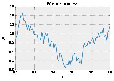
37 Simulation of Wiener Process

38 The upshot The sum 1 T yt 1 ɛ t convergences to a stochastic integral; i.e., Suppose that y t = y t 1 + ɛ t, where ɛ t iid(0, σ 2 ) and y 0 = 0. Then 1 yt 1 ɛ t = W (s)dw (s) σ T 2 where W (s) denotes a standard Wiener process. we can use this to develop tests!

39 Theorem Suppose that y t = φy t 1 + ɛ t, where ɛ t iid(0, σ 2 ), φ = 1, and y 0 = 0. The sampling distribution of the OLS estimator ˆφ T of the autoregressive parameter φ = 1 and the sampling distribution of the corresponding $t$-statistic have the following asymptotic approximations z( ˆφ T ) = t( ˆφ T ) = 1 (W 1) 2 (1)2 1 W ds 0 (s)2 1 (W 1) 2 [ (1)2 1 W ds 0 (s)2 ] 1/2 (12) (13) where W (s) denotes a standard Wiener process.