Econometría 2: Análisis de series de Tiempo
|
|
|
- Hugo Jordan Walton
- 5 years ago
- Views:
Transcription
1 Econometría 2: Análisis de series de Tiempo Karoll GOMEZ Segundo semestre 2016
2 IX. Vector Time Series Models
3 VARMA Models A.
4 1. Motivation: The vector autoregression (VAR) model is one of the most successful, flexible, and easy to use models for the analysis of multivariate time series. It is a natural extension of the univariate autoregressive model to dynamic multivariate time series. Has proven to be especially useful for describing the dynamic behavior of economic and financial time series, and for forecasting. It often provides superior forecasts to those from univariate time series models and elaborate theory-based simultaneous equations models.
5 Famous papers are Chris Sims s paper Macroeconomics and Reality (ECTA, 1980) and Stock and Watson paper Vector Autoregressions (JEP, 2001). Vector autoregressive models are a statistical tool to address the following tasks: Describe and summarize economic time series Make forecasts Recover the true structure of the macroeconomy from the data Advise macroeconomic policymakers In consequence, this analysis is commonly named as Macroeconometrics A VAR can help us answering the following questions:
6 Example 1 Problem: You want to study a sales performance for a company. Research Question: Is there a relationship between the amounts a firm spends on advertisement and sales revenue and volume? Goal: 3. To establish the relationship between advertising and sales revenue and volume Variables: sales revenue (R), sales volume (S), prices (P), sales force (F ) and advertising expenditure (E).
7 Example 2 Consider three variables: real GDP growth ( Y ), inflation (π) and the policy rate (r) A VAR can help us answering the following questions: 1. What is the dynamic behavior of these variables? How do these variables interact? 2. What is the profile of GDP conditional on a specific future path for the policy rate? 3. What is the effect of a monetary policy shock on GDP and inflation? 4. What has been the contribution of monetary policy shocks to the behavior of GDP over time?
8 1.A) What is a Vector Autoregression (VAR)?
9
10 1.B) The general form of the stationary structural VAR(p) model
11 2. Structural and Reduce form of a VAR The VAR has a very important role as a statistical model that underlies identified structural econometric models (endogenous system). However, we can write the model in a reduced form, ie stationary reduced VAR
12 The structural innovations:
13 What is a variance-covariance matrix? (Reminder)
14 Why is it called structural VAR?
15 Why is it called stationary VAR?
16 Example Structural VARs potentially answers many interesting questions
17 However... the estimation of structural VARs is problematic
18 How to solve the problem?
19
20 The reduced-form VAR
21 3. VAR stability (stationarity): DEFINITION 12: A stable VAR(p) process is stationary and ergodic with time invariant means, variances, and autocovariances. Two ways to check stationarity: 3.1 lag-operator (B) representation 3.2. System representation 3.2.1) Using the system of linear equations form 3.2.2) Using matrix form
22 3.1 lag-operator (B) representation Considering a VAR(1) model: x t = Fx t 1 + ɛ t x t Fx t 1 = ɛ t (I FB)x t = ɛ t Φ(B)x t = ɛ t VAR(1) is invertible For the process to be stationary, the zeros (roots) of the determinant equation I FB must be outside the unit circle.
23 The zeros of I FB are related to the eigenvalues of F Let be λ = λ 1,..., λ m the eigenvalues and H = h 1,..., h m the associated eigenvectors of F, such that: Thus FH =HΛ F =HΛH 1 I FB = I HΛH 1 B = I HΛBH 1 = I ΛB =Π m i=1(1 λ i B) Hence, the zeros of I FB lie outside the unit circle iff all eigenvalues λ i lies inside the unit circle, ie λ i < 1.
24 3.2. System representation 3.2.1) System of linear equations form: Consider a bivariate VAR(1) model:
25
26
27
28
29 3.2.2) The (companion) matrix form
30

31 In other words, λ i < 1
32 For the VAR(p) Model
33
34 where:
35 Nonstationarity VAR models: As we already know, in time series analysis is very common to observe series that exhibit nonstationary behavior The way to reduce nonstationary to stationary series is by differencing A natural extension (of the univariate case) to the VAR process is: Φ(B)(I IB) d Z t = ɛ t
36 Remarks for nonstationary VAR models: Orders for the differencing for each component series could be the same or not. When the differencing order for each component series could be the same and the linear combination of nonstationary series is stationary, then they are cointegrated.
37 4. Forecasting
38
39
40
41
42 5. Impulse-response function (IRFs) Impulse responses trace out the response of current and future values of each of the variables to a one-unit increase (or to a one-standard deviation increase, when the scale matters) in the current value of one of the VAR errors, assuming that this error returns to zero in subsequent periods and that all other errors are equal to zero.
43 Characteristics: The implied thought experiment of changing one error while holding the others constant makes most sense when the errors are uncorrelated across equations, so impulse responses are typically calculated for recursive and structural VARs.
44 Example 1: Considering the bivariate VAR as we already seen, we can write where
45
46 Characteristics (continued): IRFs is based on the VMA( ) representation of VAR(p) model. the VMA representation is an especially useful tool to examine the interaction between variable in the VAR
47 Considering the model VAR(p):
48
49 In other words, the matrix Ψ s collects the marginal effects of the innovation in the system on to ɛ, where: ψ ij,s = y i,t+s ɛ j,t holding all other innovations at all other dates constant. The function that evaluates those derivatives for s > 0 is called IRFs.
50 Remarks: If the correlations are high, it doesn t make much sense to ask what if ε 1,t has a unit impulse with no change in ε 2,t since both come usually at the same time. For impulse response analysis, it is therefore desirable to express the VAR in such a way that the shocks become orthogonal, (that is, the ε i s,t are uncorrelated). Additionally it is convenient to rescale the shocks so that they have a unit variance. In consequence, we need to compute the orthogonalization of correlated shocks in the original VAR. One generally used method is to use Cholesky decomposition for matriz Σ ε.
51 Choleski decomposition:
52
53
54
55 Example 2: We can calculate the IRF s to a unit shock of ε once we know A 1. Suppose we are interested in tracing the dynamics to a shock to the first variable in a two variable VAR: Thus ε 0 = [1, 0, 0] x 0 =A 1 ε t for s = 0 x s =A 1 x s 1 for s > 0 To summarize, the impulse response function is a practical way of representing the behavior over time of x in response to shocks to the vector ε.
56 Example Data are on: P=100xlog(GDP deflator), Y=100xlog(GDP), M=M2, R= Fed Funds Rate, on US quarterly data running from 1960 to We estimate a VAR(4).
57
58 Remember that: Impulse responses trace out the response of current and future values of each of the variables to a unit increase in the current value of one of the VAR structural errors, assuming that this error returns to zero thereafter.
59
60 We observe that:
61 6. Forecast error variance decomposition (FEVD) Variance decomposition can tell a researcher the percentage of the fluctuation in a time series attributable to other variables at select time horizons. In other words, tell us the proportion of the movements in a variable due to is own shocks vs the shocks to the other variables Thus, the variance decomposition provides information about the relative importance of each random innovation in affecting the variables in the VAR. In addition it can indicate which variables have short-term and long-term impacts on another variable of interest.
62 Example 3: Given the structural model:. Φ(B)x t = ε t The VMA representation is given by x t = Ψ 0 ε t + Ψ 1 ε t 1 + Ψ 2 ε t and the error in forecasting x t in the future is, for each horizon s: x t E[x t+s ] = Ψ 0 ε t+s + Ψ 1 ε t+s 1 + Ψ 2 ε t+s Ψ s 1 ε t+1 from which the variance of the forecasting error is: var(x t E[x t+s ]) = Ψ 0 Σ ε Ψ 0 + Ψ 1 Σ ε Ψ Ψ s 1 Σ ε Ψ s 1
63 Now defining e t+s = var(x t E[x t+s ]), and given that: 1. the shocks are both serially and contemporaneously uncorrelated 2. all shock components have unit variance This implies:
64 Comparing this to the sum of innovation responses, we get a relative measure: How important variable j s innovations are in the explaining the variation in variable i at different step-ahead forecasts, i.e., In other words, we compute the share of the total variance of the forecast error for each variable attributable to the variance of each structural shock.
65 In summary: Thus, while impulse response functions traces the effects of a shock to one endogenous variable on to the other variables in the VAR, variance decomposition separates the variation in an endogenous variable into the component shocks to the VAR.
66 Example FEVD (in %) OF NICARAGUAS INFLATION RATE
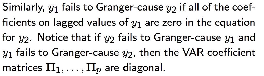
67 7. Granger causality One of the main uses of VAR models is forecasting. The following intuitive notion of a variable s forecasting ability is due to Granger (1969). If a variable, or group of variables, y 1 is found to be helpful for predicting another variable, or group of variables, y2 then y 1 is said to Granger-cause y 2 ; otherwise it is said to fail to Granger-cause y2. The notion of Granger causality does not imply true causality. It only implies forecasting ability.
68 In other words: A variable y 1 fails to Granger-causes y 2 if y 2 CAN NOT be better predicted using the histories of both y 1 and y 2, than it can using the history of y 2 alone.
69 Example: Bivariate VAR model
70
71 Formally, Which correspond to an invertible VMA(1) process: Z t = C + Θ(B)u t :
72
73 In other words, this corresponds to the restrictions that all cross-lags coefficients are all zeros which can be tested by traditional F test. For instance, for the following VAR(p) model: y t =a 1 y t 1 + a 2 y t a p y t p + b 1 x t 1 + b 2 x t b p x t p + ε y,t x t =c 1 y t 1 + c 2 y t c p y t p + d 1 x t 1 + d 2 x t d p x t p + ε x,t x does not Granger-cause y H0 :b 1 = b 2 =... = b p = 0 H1 :b 1 = b 2 =... = b p 0 y does not Granger-cause x H0 :c 1 = c 2 =... = c p = 0 H1 :c 1 = c 2 =... = c p 0
74 Conceptually, the idea has several components: 1. Temporality: Only past values of x can cause y. 2. Exogeneity: Sims (1972) points out that a necessary condition for x to be exogenous of y is that x fails to Granger-cause y. 3. Independence: Similarly, variables x and y are only independent if both fail to Granger-cause the other.
75 Example: Trivariate VAR model

76 8. Estimation Note that if the disturbances in one equation are for example autocorrelated, the theory does not apply. Then need IV estimators, including GMM
77 Traditionally, VAR models are designed for stationary variables without time trends. So, first we need to be sure vector series must be stationary or properly stationarized. How do we test the VAR assumptions?
78 1. Determination of p (specification testing) Information criteria: The general approach is to fit VAR(p) models with orders p = 0,..., pmax and choose the value of p which minimizes some model selection criteria: Schwarz (SC), Hannan-Quin (HQ) and Akaike (AIC). Start with a large p and test successively that the coefficients of the largest lag in the VAR is zero: i.e., a sequence of F-tests. Under-specification of p might result in residuals that are autocorrelated. Information criteria and sequence of tests can of course be combined
79 REMARKS: AIC criterion asymptotically overestimates the order with positive probability BIC and HQ criteria estimate the order consistently, under fairly general conditions, if the true order p is less than or equal to pmax.
80 2. Testing assumptions about ε it (mis-specifiation testing) Since each equation is estimated by OLS, we can use a test-battery: autoregresive autocorrelation, ARCH disturbance, White tests of heteroskedasticity, non-normality tests. Note the degrees of freedom tend to be very large for these tests, so even if the size of the test is OK, mis-specification may be hidden (due to low power of test). Significant departures from the hypothesis of Gaussian disturbances can often be resolved by: Larger p Increase the dimension of the VAR: more variables in the yt vector. Introduce exogenous stochastic explanatory variables: VAR-X model, conditional or partial model. Introduce deterministic variables in the VAR.
81 The economic relevance of the statistically well specified VAR is a matter in itself. Little help if p is set so large that there are no degrees of freedom left, or if VAR-X introduce variables that are difficult to rationalize or interpret theoretically or historically. May then want to estimate simpler model with GMM for each equation instead.
82 How to build flexibility into the VAR?
83
84 VARMA Models B. VARMA Models
85 VARMA Models Considering the following VARMA(p,q) model: Φ(B)Z t = Θ(B)u t where Φ(B) =F 1 B + F 2 B F p B p Θ(B) =Θ 1 B + Θ 2 B Θ p B p
Multivariate Time Series Analysis and Its Applications [Tsay (2005), chapter 8]
![Multivariate Time Series Analysis and Its Applications [Tsay (2005), chapter 8]](/thumbs/77/75858385.jpg "Multivariate Time Series Analysis and Its Applications [Tsay (2005), chapter 8]") 1 Multivariate Time Series Analysis and Its Applications [Tsay (2005), chapter 8] Insights: Price movements in one market can spread easily and instantly to another market [economic globalization and internet
1 Multivariate Time Series Analysis and Its Applications [Tsay (2005), chapter 8] Insights: Price movements in one market can spread easily and instantly to another market [economic globalization and internet
A Primer on Vector Autoregressions
 A Primer on Vector Autoregressions Ambrogio Cesa-Bianchi VAR models 1 [DISCLAIMER] These notes are meant to provide intuition on the basic mechanisms of VARs As such, most of the material covered here
Vector autoregressions, VAR
 1 / 45 Vector autoregressions, VAR Chapter 2 Financial Econometrics Michael Hauser WS17/18 2 / 45 Content Cross-correlations VAR model in standard/reduced form Properties of VAR(1), VAR(p) Structural VAR,
Title. Description. var intro Introduction to vector autoregressive models
 Title var intro Introduction to vector autoregressive models Description Stata has a suite of commands for fitting, forecasting, interpreting, and performing inference on vector autoregressive (VAR) models
Vector Auto-Regressive Models
 Vector Auto-Regressive Models Laurent Ferrara 1 1 University of Paris Nanterre M2 Oct. 2018 Overview of the presentation 1. Vector Auto-Regressions Definition Estimation Testing 2. Impulse responses functions
A primer on Structural VARs
 A primer on Structural VARs Claudia Foroni Norges Bank 10 November 2014 Structural VARs 1/ 26 Refresh: what is a VAR? VAR (p) : where y t K 1 y t = ν + B 1 y t 1 +... + B p y t p + u t, (1) = ( y 1t...
VAR Models and Applications
 VAR Models and Applications Laurent Ferrara 1 1 University of Paris West M2 EIPMC Oct. 2016 Overview of the presentation 1. Vector Auto-Regressions Definition Estimation Testing 2. Impulse responses functions
Multivariate Time Series: VAR(p) Processes and Models
 Processes and Models") Multivariate Time Series: VAR(p) Processes and Models A VAR(p) model, for p > 0 is X t = φ 0 + Φ 1 X t 1 + + Φ p X t p + A t, where X t, φ 0, and X t i are k-vectors, Φ 1,..., Φ p are k k matrices, with
Multivariate Time Series: VAR(p) Processes and Models A VAR(p) model, for p > 0 is X t = φ 0 + Φ 1 X t 1 + + Φ p X t p + A t, where X t, φ 0, and X t i are k-vectors, Φ 1,..., Φ p are k k matrices, with
Econ 423 Lecture Notes: Additional Topics in Time Series 1
 Econ 423 Lecture Notes: Additional Topics in Time Series 1 John C. Chao April 25, 2017 1 These notes are based in large part on Chapter 16 of Stock and Watson (2011). They are for instructional purposes
Financial Econometrics
 Financial Econometrics Multivariate Time Series Analysis: VAR Gerald P. Dwyer Trinity College, Dublin January 2013 GPD (TCD) VAR 01/13 1 / 25 Structural equations Suppose have simultaneous system for supply
Topic 4 Unit Roots. Gerald P. Dwyer. February Clemson University
 Topic 4 Unit Roots Gerald P. Dwyer Clemson University February 2016 Outline 1 Unit Roots Introduction Trend and Difference Stationary Autocorrelations of Series That Have Deterministic or Stochastic Trends
Time Series Analysis. James D. Hamilton PRINCETON UNIVERSITY PRESS PRINCETON, NEW JERSEY
 Time Series Analysis James D. Hamilton PRINCETON UNIVERSITY PRESS PRINCETON, NEW JERSEY & Contents PREFACE xiii 1 1.1. 1.2. Difference Equations First-Order Difference Equations 1 /?th-order Difference
Stationarity and Cointegration analysis. Tinashe Bvirindi
 Stationarity and Cointegration analysis By Tinashe Bvirindi tbvirindi@gmail.com layout Unit root testing Cointegration Vector Auto-regressions Cointegration in Multivariate systems Introduction Stationarity
Multivariate forecasting with VAR models
 Multivariate forecasting with VAR models Franz Eigner University of Vienna UK Econometric Forecasting Prof. Robert Kunst 16th June 2009 Overview Vector autoregressive model univariate forecasting multivariate
Oil price and macroeconomy in Russia. Abstract
 Oil price and macroeconomy in Russia Katsuya Ito Fukuoka University Abstract In this note, using the VEC model we attempt to empirically investigate the effects of oil price and monetary shocks on the
ECON 4160, Lecture 11 and 12
 ECON 4160, 2016. Lecture 11 and 12 Co-integration Ragnar Nymoen Department of Economics 9 November 2017 1 / 43 Introduction I So far we have considered: Stationary VAR ( no unit roots ) Standard inference
Structural VAR Models and Applications
 Structural VAR Models and Applications Laurent Ferrara 1 1 University of Paris Nanterre M2 Oct. 2018 SVAR: Objectives Whereas the VAR model is able to capture efficiently the interactions between the different
Lecture 2: Univariate Time Series
 Lecture 2: Univariate Time Series Analysis: Conditional and Unconditional Densities, Stationarity, ARMA Processes Prof. Massimo Guidolin 20192 Financial Econometrics Spring/Winter 2017 Overview Motivation:
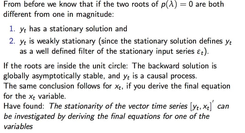
B y t = γ 0 + Γ 1 y t + ε t B(L) y t = γ 0 + ε t ε t iid (0, D) D is diagonal
 y t = γ 0 + ε t ε t iid (0, D) D is diagonal") Structural VAR Modeling for I(1) Data that is Not Cointegrated Assume y t =(y 1t,y 2t ) 0 be I(1) and not cointegrated. That is, y 1t and y 2t are both I(1) and there is no linear combination of y 1t and
Structural VAR Modeling for I(1) Data that is Not Cointegrated Assume y t =(y 1t,y 2t ) 0 be I(1) and not cointegrated. That is, y 1t and y 2t are both I(1) and there is no linear combination of y 1t and
Lesson 17: Vector AutoRegressive Models
 Dipartimento di Ingegneria e Scienze dell Informazione e Matematica Università dell Aquila, umberto.triacca@ec.univaq.it Vector AutoRegressive models The extension of ARMA models into a multivariate framework
Time Series Analysis. James D. Hamilton PRINCETON UNIVERSITY PRESS PRINCETON, NEW JERSEY
 Time Series Analysis James D. Hamilton PRINCETON UNIVERSITY PRESS PRINCETON, NEW JERSEY PREFACE xiii 1 Difference Equations 1.1. First-Order Difference Equations 1 1.2. pth-order Difference Equations 7
Vector Autoregression
 Vector Autoregression Prabakar Rajasekaran December 13, 212 1 Introduction Vector autoregression (VAR) is an econometric model used to capture the evolution and the interdependencies between multiple time
Econometría 2: Análisis de series de Tiempo
 Econometría 2: Análisis de series de Tiempo Karoll GOMEZ kgomezp@unal.edu.co http://karollgomez.wordpress.com Segundo semestre 2016 II. Basic definitions A time series is a set of observations X t, each
2.5 Forecasting and Impulse Response Functions
 2.5 Forecasting and Impulse Response Functions Principles of forecasting Forecast based on conditional expectations Suppose we are interested in forecasting the value of y t+1 based on a set of variables
New Introduction to Multiple Time Series Analysis
 Helmut Lütkepohl New Introduction to Multiple Time Series Analysis With 49 Figures and 36 Tables Springer Contents 1 Introduction 1 1.1 Objectives of Analyzing Multiple Time Series 1 1.2 Some Basics 2
The regression model with one stochastic regressor (part II)
") The regression model with one stochastic regressor (part II) 3150/4150 Lecture 7 Ragnar Nymoen 6 Feb 2012 We will finish Lecture topic 4: The regression model with stochastic regressor We will first look
The regression model with one stochastic regressor (part II) 3150/4150 Lecture 7 Ragnar Nymoen 6 Feb 2012 We will finish Lecture topic 4: The regression model with stochastic regressor We will first look
Topic 3. Recursive multivariate models. Exogenous variables. Single-equation models. Prof. A.Espasa
 Topic 3 Recursive multivariate models. Exogenous variables. Single-equation models. Prof. A.Espasa INFORMATION SETS DATA SETS DATA SET UNIVARIATE MULTIVARIATE ENDOGENOUS EXOGENOUS Consider only the time
Lecture 7a: Vector Autoregression (VAR)
") Lecture 7a: Vector Autoregression (VAR) 1 Big Picture We are done with univariate time series analysis Now we switch to multivariate analysis, that is, studying several time series simultaneously. VAR
Lecture 7a: Vector Autoregression (VAR) 1 Big Picture We are done with univariate time series analysis Now we switch to multivariate analysis, that is, studying several time series simultaneously. VAR
Structural VARs II. February 17, 2016
 Structural VARs II February 17, 216 Structural VARs Today: Long-run restrictions Two critiques of SVARs Blanchard and Quah (1989), Rudebusch (1998), Gali (1999) and Chari, Kehoe McGrattan (28). Recap:
A Non-Parametric Approach of Heteroskedasticity Robust Estimation of Vector-Autoregressive (VAR) Models
 Models") Journal of Finance and Investment Analysis, vol.1, no.1, 2012, 55-67 ISSN: 2241-0988 (print version), 2241-0996 (online) International Scientific Press, 2012 A Non-Parametric Approach of Heteroskedasticity
Journal of Finance and Investment Analysis, vol.1, no.1, 2012, 55-67 ISSN: 2241-0988 (print version), 2241-0996 (online) International Scientific Press, 2012 A Non-Parametric Approach of Heteroskedasticity
A. Recursively orthogonalized. VARs
 Orthogonalized VARs A. Recursively orthogonalized VAR B. Variance decomposition C. Historical decomposition D. Structural interpretation E. Generalized IRFs 1 A. Recursively orthogonalized Nonorthogonal
Cointegrated VAR s. Eduardo Rossi University of Pavia. November Rossi Cointegrated VAR s Financial Econometrics / 56
 Cointegrated VAR s Eduardo Rossi University of Pavia November 2013 Rossi Cointegrated VAR s Financial Econometrics - 2013 1 / 56 VAR y t = (y 1t,..., y nt ) is (n 1) vector. y t VAR(p): Φ(L)y t = ɛ t The
Lecture 7a: Vector Autoregression (VAR)
") Lecture 7a: Vector Autoregression (VAR) 1 2 Big Picture We are done with univariate time series analysis Now we switch to multivariate analysis, that is, studying several time series simultaneously. VAR
Lecture 7a: Vector Autoregression (VAR) 1 2 Big Picture We are done with univariate time series analysis Now we switch to multivariate analysis, that is, studying several time series simultaneously. VAR
Simultaneous Equation Models Learning Objectives Introduction Introduction (2) Introduction (3) Solving the Model structural equations
 Introduction (3) Solving the Model structural equations") Simultaneous Equation Models. Introduction: basic definitions 2. Consequences of ignoring simultaneity 3. The identification problem 4. Estimation of simultaneous equation models 5. Example: IS LM model
Simultaneous Equation Models. Introduction: basic definitions 2. Consequences of ignoring simultaneity 3. The identification problem 4. Estimation of simultaneous equation models 5. Example: IS LM model
ECON 4160, Spring term Lecture 12
 ECON 4160, Spring term 2013. Lecture 12 Non-stationarity and co-integration 2/2 Ragnar Nymoen Department of Economics 13 Nov 2013 1 / 53 Introduction I So far we have considered: Stationary VAR, with deterministic
Factor models. March 13, 2017
 Factor models March 13, 2017 Factor Models Macro economists have a peculiar data situation: Many data series, but usually short samples How can we utilize all this information without running into degrees
Econometric Forecasting
 Robert M. Kunst robert.kunst@univie.ac.at University of Vienna and Institute for Advanced Studies Vienna October 1, 2014 Outline Introduction Model-free extrapolation Univariate time-series models Trend
Lecture 1: Information and Structural VARs
 Lecture 1: Information and Structural VARs Luca Gambetti 1 1 Universitat Autònoma de Barcelona LBS, May 6-8 2013 Introduction The study of the dynamic effects of economic shocks is one of the key applications
Identifying Aggregate Liquidity Shocks with Monetary Policy Shocks: An Application using UK Data
 Identifying Aggregate Liquidity Shocks with Monetary Policy Shocks: An Application using UK Data Michael Ellington and Costas Milas Financial Services, Liquidity and Economic Activity Bank of England May
Class 4: VAR. Macroeconometrics - Fall October 11, Jacek Suda, Banque de France
 VAR IRF Short-run Restrictions Long-run Restrictions Granger Summary Jacek Suda, Banque de France October 11, 2013 VAR IRF Short-run Restrictions Long-run Restrictions Granger Summary Outline Outline:
FinQuiz Notes
 Reading 9 A time series is any series of data that varies over time e.g. the quarterly sales for a company during the past five years or daily returns of a security. When assumptions of the regression
Factor models. May 11, 2012
 Factor models May 11, 2012 Factor Models Macro economists have a peculiar data situation: Many data series, but usually short samples How can we utilize all this information without running into degrees
Vector Autogregression and Impulse Response Functions
 Chapter 8 Vector Autogregression and Impulse Response Functions 8.1 Vector Autogregressions Consider two sequences {y t } and {z t }, where the time path of {y t } is affected by current and past realizations
1 Teaching notes on structural VARs.
 Bent E. Sørensen November 8, 2016 1 Teaching notes on structural VARs. 1.1 Vector MA models: 1.1.1 Probability theory The simplest to analyze, estimation is a different matter time series models are the
When Do Wold Orderings and Long-Run Recursive Identifying Restrictions Yield Identical Results?
 Preliminary and incomplete When Do Wold Orderings and Long-Run Recursive Identifying Restrictions Yield Identical Results? John W Keating * University of Kansas Department of Economics 334 Snow Hall Lawrence,
Booth School of Business, University of Chicago Business 41914, Spring Quarter 2017, Mr. Ruey S. Tsay. Solutions to Midterm
 Booth School of Business, University of Chicago Business 41914, Spring Quarter 017, Mr Ruey S Tsay Solutions to Midterm Problem A: (51 points; 3 points per question) Answer briefly the following questions
Brief Sketch of Solutions: Tutorial 3. 3) unit root tests
 unit root tests") Brief Sketch of Solutions: Tutorial 3 3) unit root tests.5.4.4.3.3.2.2.1.1.. -.1 -.1 -.2 -.2 -.3 -.3 -.4 -.4 21 22 23 24 25 26 -.5 21 22 23 24 25 26.8.2.4. -.4 - -.8 - - -.12 21 22 23 24 25 26 -.2 21 22
Brief Sketch of Solutions: Tutorial 3 3) unit root tests.5.4.4.3.3.2.2.1.1.. -.1 -.1 -.2 -.2 -.3 -.3 -.4 -.4 21 22 23 24 25 26 -.5 21 22 23 24 25 26.8.2.4. -.4 - -.8 - - -.12 21 22 23 24 25 26 -.2 21 22
G. S. Maddala Kajal Lahiri. WILEY A John Wiley and Sons, Ltd., Publication
 G. S. Maddala Kajal Lahiri WILEY A John Wiley and Sons, Ltd., Publication TEMT Foreword Preface to the Fourth Edition xvii xix Part I Introduction and the Linear Regression Model 1 CHAPTER 1 What is Econometrics?
Econometrics II. Seppo Pynnönen. Spring Department of Mathematics and Statistics, University of Vaasa, Finland
 Department of Mathematics and Statistics, University of Vaasa, Finland Spring 218 Part VI Vector Autoregression As of Feb 21, 218 1 Vector Autoregression (VAR) Background The Model Defining the order of
Vector Autoregressive Model. Vector Autoregressions II. Estimation of Vector Autoregressions II. Estimation of Vector Autoregressions I.
 Vector Autoregressive Model Vector Autoregressions II Empirical Macroeconomics - Lect 2 Dr. Ana Beatriz Galvao Queen Mary University of London January 2012 A VAR(p) model of the m 1 vector of time series
ECON 4160: Econometrics-Modelling and Systems Estimation Lecture 9: Multiple equation models II
 ECON 4160: Econometrics-Modelling and Systems Estimation Lecture 9: Multiple equation models II Ragnar Nymoen Department of Economics University of Oslo 9 October 2018 The reference to this lecture is:
ECON3327: Financial Econometrics, Spring 2016
 ECON3327: Financial Econometrics, Spring 2016 Wooldridge, Introductory Econometrics (5th ed, 2012) Chapter 11: OLS with time series data Stationary and weakly dependent time series The notion of a stationary
Notes on Time Series Modeling
 Notes on Time Series Modeling Garey Ramey University of California, San Diego January 17 1 Stationary processes De nition A stochastic process is any set of random variables y t indexed by t T : fy t g
9) Time series econometrics
 Time series econometrics") 30C00200 Econometrics 9) Time series econometrics Timo Kuosmanen Professor Management Science http://nomepre.net/index.php/timokuosmanen 1 Macroeconomic data: GDP Inflation rate Examples of time series
30C00200 Econometrics 9) Time series econometrics Timo Kuosmanen Professor Management Science http://nomepre.net/index.php/timokuosmanen 1 Macroeconomic data: GDP Inflation rate Examples of time series
Identifying the Monetary Policy Shock Christiano et al. (1999)
") Identifying the Monetary Policy Shock Christiano et al. (1999) The question we are asking is: What are the consequences of a monetary policy shock a shock which is purely related to monetary conditions
Identifying the Monetary Policy Shock Christiano et al. (1999) The question we are asking is: What are the consequences of a monetary policy shock a shock which is purely related to monetary conditions
10. Time series regression and forecasting
 10. Time series regression and forecasting Key feature of this section: Analysis of data on a single entity observed at multiple points in time (time series data) Typical research questions: What is the
Booth School of Business, University of Chicago Business 41914, Spring Quarter 2013, Mr. Ruey S. Tsay. Midterm
 Booth School of Business, University of Chicago Business 41914, Spring Quarter 2013, Mr. Ruey S. Tsay Midterm Chicago Booth Honor Code: I pledge my honor that I have not violated the Honor Code during
Econ 623 Econometrics II Topic 2: Stationary Time Series
 1 Introduction Econ 623 Econometrics II Topic 2: Stationary Time Series In the regression model we can model the error term as an autoregression AR(1) process. That is, we can use the past value of the
EC408 Topics in Applied Econometrics. B Fingleton, Dept of Economics, Strathclyde University
 EC48 Topics in Applied Econometrics B Fingleton, Dept of Economics, Strathclyde University Applied Econometrics What is spurious regression? How do we check for stochastic trends? Cointegration and Error
1 Teaching notes on structural VARs.
 Bent E. Sørensen February 22, 2007 1 Teaching notes on structural VARs. 1.1 Vector MA models: 1.1.1 Probability theory The simplest (to analyze, estimation is a different matter) time series models are
Introduction to Eco n o m et rics
 2008 AGI-Information Management Consultants May be used for personal purporses only or by libraries associated to dandelon.com network. Introduction to Eco n o m et rics Third Edition G.S. Maddala Formerly
at least 50 and preferably 100 observations should be available to build a proper model
 III Box-Jenkins Methods 1. Pros and Cons of ARIMA Forecasting a) need for data at least 50 and preferably 100 observations should be available to build a proper model used most frequently for hourly or
Stochastic Trends & Economic Fluctuations
 Stochastic Trends & Economic Fluctuations King, Plosser, Stock & Watson (AER, 1991) Cesar E. Tamayo Econ508 - Economics - Rutgers November 14, 2011 Cesar E. Tamayo Stochastic Trends & Economic Fluctuations
A Guide to Modern Econometric:
 A Guide to Modern Econometric: 4th edition Marno Verbeek Rotterdam School of Management, Erasmus University, Rotterdam B 379887 )WILEY A John Wiley & Sons, Ltd., Publication Contents Preface xiii 1 Introduction
Autoregressive models with distributed lags (ADL)
") Autoregressive models with distributed lags (ADL) It often happens than including the lagged dependent variable in the model results in model which is better fitted and needs less parameters. It can be
Autoregressive models with distributed lags (ADL) It often happens than including the lagged dependent variable in the model results in model which is better fitted and needs less parameters. It can be
Chapter 2. Some basic tools. 2.1 Time series: Theory Stochastic processes
 Chapter 2 Some basic tools 2.1 Time series: Theory 2.1.1 Stochastic processes A stochastic process is a sequence of random variables..., x 0, x 1, x 2,.... In this class, the subscript always means time.
Empirical Market Microstructure Analysis (EMMA)
") Empirical Market Microstructure Analysis (EMMA) Lecture 3: Statistical Building Blocks and Econometric Basics Prof. Dr. Michael Stein michael.stein@vwl.uni-freiburg.de Albert-Ludwigs-University of Freiburg
Empirical Market Microstructure Analysis (EMMA) Lecture 3: Statistical Building Blocks and Econometric Basics Prof. Dr. Michael Stein michael.stein@vwl.uni-freiburg.de Albert-Ludwigs-University of Freiburg
A Horse-Race Contest of Selected Economic Indicators & Their Potential Prediction Abilities on GDP
 A Horse-Race Contest of Selected Economic Indicators & Their Potential Prediction Abilities on GDP Tahmoures Afshar, Woodbury University, USA ABSTRACT This paper empirically investigates, in the context
Time-Varying Vector Autoregressive Models with Structural Dynamic Factors
 Time-Varying Vector Autoregressive Models with Structural Dynamic Factors Paolo Gorgi, Siem Jan Koopman, Julia Schaumburg http://sjkoopman.net Vrije Universiteit Amsterdam School of Business and Economics
Chapter 5. Analysis of Multiple Time Series. 5.1 Vector Autoregressions
 Chapter 5 Analysis of Multiple Time Series Note: The primary references for these notes are chapters 5 and 6 in Enders (2004). An alternative, but more technical treatment can be found in chapters 10-11
Augmenting our AR(4) Model of Inflation. The Autoregressive Distributed Lag (ADL) Model
 Model of Inflation. The Autoregressive Distributed Lag (ADL) Model") Augmenting our AR(4) Model of Inflation Adding lagged unemployment to our model of inflationary change, we get: Inf t =1.28 (0.31) Inf t 1 (0.39) Inf t 2 +(0.09) Inf t 3 (0.53) (0.09) (0.09) (0.08) (0.08)
Augmenting our AR(4) Model of Inflation Adding lagged unemployment to our model of inflationary change, we get: Inf t =1.28 (0.31) Inf t 1 (0.39) Inf t 2 +(0.09) Inf t 3 (0.53) (0.09) (0.09) (0.08) (0.08)
Dynamic Time Series Regression: A Panacea for Spurious Correlations
 International Journal of Scientific and Research Publications, Volume 6, Issue 10, October 2016 337 Dynamic Time Series Regression: A Panacea for Spurious Correlations Emmanuel Alphonsus Akpan *, Imoh
Prof. Dr. Roland Füss Lecture Series in Applied Econometrics Summer Term Introduction to Time Series Analysis
 Introduction to Time Series Analysis 1 Contents: I. Basics of Time Series Analysis... 4 I.1 Stationarity... 5 I.2 Autocorrelation Function... 9 I.3 Partial Autocorrelation Function (PACF)... 14 I.4 Transformation
Booth School of Business, University of Chicago Business 41914, Spring Quarter 2017, Mr. Ruey S. Tsay Midterm
 Booth School of Business, University of Chicago Business 41914, Spring Quarter 2017, Mr. Ruey S. Tsay Midterm Chicago Booth Honor Code: I pledge my honor that I have not violated the Honor Code during
Autoregressive distributed lag models
 Introduction In economics, most cases we want to model relationships between variables, and often simultaneously. That means we need to move from univariate time series to multivariate. We do it in two
MFx Macroeconomic Forecasting
 MFx Macroeconomic Forecasting Structural Vector Autoregressive Models Part II IMFx This training material is the property of the International Monetary Fund (IMF) and is intended for use in IMF Institute
10) Time series econometrics
 Time series econometrics") 30C00200 Econometrics 10) Time series econometrics Timo Kuosmanen Professor, Ph.D. 1 Topics today Static vs. dynamic time series model Suprious regression Stationary and nonstationary time series Unit
30C00200 Econometrics 10) Time series econometrics Timo Kuosmanen Professor, Ph.D. 1 Topics today Static vs. dynamic time series model Suprious regression Stationary and nonstationary time series Unit
11. Further Issues in Using OLS with TS Data
 11. Further Issues in Using OLS with TS Data With TS, including lags of the dependent variable often allow us to fit much better the variation in y Exact distribution theory is rarely available in TS applications,
1. Shocks. This version: February 15, Nr. 1
 1. Shocks This version: February 15, 2006 Nr. 1 1.3. Factor models What if there are more shocks than variables in the VAR? What if there are only a few underlying shocks, explaining most of fluctuations?
Cointegrated VARIMA models: specification and. simulation
 Cointegrated VARIMA models: specification and simulation José L. Gallego and Carlos Díaz Universidad de Cantabria. Abstract In this note we show how specify cointegrated vector autoregressive-moving average
Vector error correction model, VECM Cointegrated VAR
 1 / 58 Vector error correction model, VECM Cointegrated VAR Chapter 4 Financial Econometrics Michael Hauser WS17/18 2 / 58 Content Motivation: plausible economic relations Model with I(1) variables: spurious
2. Multivariate ARMA
 2. Multivariate ARMA JEM 140: Quantitative Multivariate Finance IES, Charles University, Prague Summer 2018 JEM 140 () 2. Multivariate ARMA Summer 2018 1 / 19 Multivariate AR I Let r t = (r 1t,..., r kt
Econometrics. 9) Heteroscedasticity and autocorrelation
 Heteroscedasticity and autocorrelation") 30C00200 Econometrics 9) Heteroscedasticity and autocorrelation Timo Kuosmanen Professor, Ph.D. http://nomepre.net/index.php/timokuosmanen Today s topics Heteroscedasticity Possible causes Testing for
30C00200 Econometrics 9) Heteroscedasticity and autocorrelation Timo Kuosmanen Professor, Ph.D. http://nomepre.net/index.php/timokuosmanen Today s topics Heteroscedasticity Possible causes Testing for
LATVIAN GDP: TIME SERIES FORECASTING USING VECTOR AUTO REGRESSION
 LATVIAN GDP: TIME SERIES FORECASTING USING VECTOR AUTO REGRESSION BEZRUCKO Aleksandrs, (LV) Abstract: The target goal of this work is to develop a methodology of forecasting Latvian GDP using ARMA (AutoRegressive-Moving-Average)
GARCH Models. Eduardo Rossi University of Pavia. December Rossi GARCH Financial Econometrics / 50
 GARCH Models Eduardo Rossi University of Pavia December 013 Rossi GARCH Financial Econometrics - 013 1 / 50 Outline 1 Stylized Facts ARCH model: definition 3 GARCH model 4 EGARCH 5 Asymmetric Models 6
Dynamic Regression Models (Lect 15)
") Dynamic Regression Models (Lect 15) Ragnar Nymoen University of Oslo 21 March 2013 1 / 17 HGL: Ch 9; BN: Kap 10 The HGL Ch 9 is a long chapter, and the testing for autocorrelation part we have already
Dynamic Regression Models (Lect 15) Ragnar Nymoen University of Oslo 21 March 2013 1 / 17 HGL: Ch 9; BN: Kap 10 The HGL Ch 9 is a long chapter, and the testing for autocorrelation part we have already
Vector Autoregression
 Vector Autoregression Jamie Monogan University of Georgia February 27, 2018 Jamie Monogan (UGA) Vector Autoregression February 27, 2018 1 / 17 Objectives By the end of these meetings, participants should
Time Series Methods. Sanjaya Desilva
 Time Series Methods Sanjaya Desilva 1 Dynamic Models In estimating time series models, sometimes we need to explicitly model the temporal relationships between variables, i.e. does X affect Y in the same
FE570 Financial Markets and Trading. Stevens Institute of Technology
 FE570 Financial Markets and Trading Lecture 5. Linear Time Series Analysis and Its Applications (Ref. Joel Hasbrouck - Empirical Market Microstructure ) Steve Yang Stevens Institute of Technology 9/25/2012
STA 6857 VAR, VARMA, VARMAX ( 5.7)
") STA 6857 VAR, VARMA, VARMAX ( 5.7) Outline 1 Multivariate Time Series Modeling 2 VAR 3 VARIMA/VARMAX Arthur Berg STA 6857 VAR, VARMA, VARMAX ( 5.7) 2/ 16 Outline 1 Multivariate Time Series Modeling 2 VAR
STA 6857 VAR, VARMA, VARMAX ( 5.7) Outline 1 Multivariate Time Series Modeling 2 VAR 3 VARIMA/VARMAX Arthur Berg STA 6857 VAR, VARMA, VARMAX ( 5.7) 2/ 16 Outline 1 Multivariate Time Series Modeling 2 VAR
Multivariate Models. Christopher Ting. Christopher Ting. April 19,
 Multivariate Models Chapter 7 of Chris Brook s Book Christopher Ting http://www.mysmu.edu/faculty/christophert/ Christopher Ting : christopherting@smu.edu.sg : 6828 0364 : LKCSB 5036 April 19, 2017 Christopher
Computational Macroeconomics. Prof. Dr. Maik Wolters Friedrich Schiller University Jena
 Computational Macroeconomics Prof. Dr. Maik Wolters Friedrich Schiller University Jena Overview Objective: Learn doing empirical and applied theoretical work in monetary macroeconomics Implementing macroeconomic
7. Integrated Processes
 7. Integrated Processes Up to now: Analysis of stationary processes (stationary ARMA(p, q) processes) Problem: Many economic time series exhibit non-stationary patterns over time 226 Example: We consider
Econometría 2: Análisis de series de Tiempo
 Econometría 2: Análisis de series de Tiempo Karoll GOMEZ kgomezp@unal.edu.co http://karollgomez.wordpress.com Segundo semestre 2016 III. Stationary models 1 Purely random process 2 Random walk (non-stationary)
A Critical Note on the Forecast Error Variance Decomposition
 A Critical Note on the Forecast Error Variance Decomposition Atilim Seymen This Version: March, 28 Preliminary: Do not cite without author s permisson. Abstract The paper questions the reasonability of
Inference in VARs with Conditional Heteroskedasticity of Unknown Form
 Inference in VARs with Conditional Heteroskedasticity of Unknown Form Ralf Brüggemann a Carsten Jentsch b Carsten Trenkler c University of Konstanz University of Mannheim University of Mannheim IAB Nuremberg
Chapter 2: Unit Roots
 Chapter 2: Unit Roots 1 Contents: Lehrstuhl für Department Empirische of Wirtschaftsforschung Empirical Research and undeconometrics II. Unit Roots... 3 II.1 Integration Level... 3 II.2 Nonstationarity
Variable Targeting and Reduction in High-Dimensional Vector Autoregressions
 Variable Targeting and Reduction in High-Dimensional Vector Autoregressions Tucker McElroy (U.S. Census Bureau) Frontiers in Forecasting February 21-23, 2018 1 / 22 Disclaimer This presentation is released
Time Series Forecasting: A Tool for Out - Sample Model Selection and Evaluation
 AMERICAN JOURNAL OF SCIENTIFIC AND INDUSTRIAL RESEARCH 214, Science Huβ, http://www.scihub.org/ajsir ISSN: 2153-649X, doi:1.5251/ajsir.214.5.6.185.194 Time Series Forecasting: A Tool for Out - Sample Model
13. Time Series Analysis: Asymptotics Weakly Dependent and Random Walk Process. Strict Exogeneity
 Outline: Further Issues in Using OLS with Time Series Data 13. Time Series Analysis: Asymptotics Weakly Dependent and Random Walk Process I. Stationary and Weakly Dependent Time Series III. Highly Persistent