Topic 3. Recursive multivariate models. Exogenous variables. Single-equation models. Prof. A.Espasa

Transcription

1 Topic 3 Recursive multivariate models. Exogenous variables. Single-equation models. Prof. A.Espasa

2 INFORMATION SETS

3 DATA SETS DATA SET UNIVARIATE MULTIVARIATE ENDOGENOUS EXOGENOUS Consider only the time series relating to the phenomena interest X t. Consider n-component time series series that can be decomposed X t. Consider the series of interest X t, y t and other K series, Z 1t,..., Z Kt with which it is related. BASIC UNIVARIATE DATA SET In time series, the frequency of data is low, usually, annual data 2 EXPANSION FOR FUNCTIONAL DISAGGREGRATION 4 EXPANSION WITH OTHER SERIES, WITH THAT DETECT AN EMPIRICAL RELATION OF DEPENDENCE 1 FREQUENCY 1 EXPANSION 3 EXPANSION FOR GEOGRAPHIC DISAGGREGRATION 5 EXPANSION WITH OTHER SERIES, WITH THAT APPLY A THEORITIC RELATION

4 Models for univariate data set. Univariate models with structure for evolution and dependence of time series. These models contain the variable determined by its past values. A stochastic finite differential equation.

5 Models for multivariate data set. Need Economic Theory in the formulation. Multiequation models. The concept of exogeneity is important in econometric model building. Exogenous variables: affect the phenomenon of interest, but in the particular case that analyzes determinations (such as the ones of parameters, forecasting, simulation), exogenous variables are not affected by those determinations. Different types of exogeneity depend on the particular analysis that is realized.

6 For multivariate data set, the variable of interest is scalar, models in principle should be multi-equation, however, single equation models can be built depending on the presence of exogenous variables. If in the explanation of a phenomenon {y t } the explanatory variables are all exogenous, multiequational model is needed to explain both y t and the remaining endogenous variables. In principle, these models are necessary for economic analysis. Single equation models for forecasting: all the explanatory variables should be strongly exogenous. For example, a model which determines the number of tourists visiting Spain in a given quarter is based on an indicator of tourist income and relative price indicators.

7 In multi-equation models, the explanatory variables can be replaced by their univariate form and can be demonstrated -see Zellner and Palm (1974) - each endogenous variable in a multi-equational model may obtain a final form corresponding to univariate model. This result justifies the use of univariate models in previous topics. Multivariate models are reduced form when the contemporary relationship between variables is not specified and is assumed in the residual covariance matrix.

8 DYNAMIC ECONOMETRIC MODELS Univariate information set - (1) Univariate models: ARI(p,d) Multivariate information sets. Proper econometric models: - (2) Single-equation models: dynamic regression models. - (3) Multiple-equation dynamic models. Complexity and utility of the above models.

9 REFERENCES A possible reference for preparation of this subject is Chapter 3 of Espasa, A. and J.R. Cancel (eds.), 1993, 1993,Métodos Cuantitativos para el Análisis de la Coyuntura Económica, Alianza Editor

10 UNIVARIATE MODELS AND QUANTITATIVE ANALYSIS IN THE FIRM. The economic reality of a firm creates variables - time series - different from each other, but are determined by the interrelationship between different variables. So, univariate ARIMA models which deal with the above issues are an initial step, that is necessary to model economic situations of the firm, but their use is very limited because they ignore the relationship between variables.

11 USES OF AN ARIMA MODEL DEALING WITH A SALE VARIABLE An ARIMA model dealing with sale of one product of a firm in a particular geographic area is useful for the structural analysis on the sale to know their characteristics trend, seasonality and cycle and know the uncertainty associated with future prospect given the past events, and so on.

12 USES OF AN ARIMA MODEL DEALING WITH A SALE VARIABLE AN ARIMA MODEL CAN BE USED TO PREDICT. In fact, the model contains the dependence of sales at a given time, in a function of the past. Thus, the dependence can be used to project the future value at time (n + h), given the past until the time n.

13 LIMITATIONS OF ARIMA MODEL DEALING WITH A SALE VARIABLE but the previous model is of limited interest in terms of planning and business management, because it does not provide more relevant structural information as the relationship between sales and other variables such as advertising campaigns, changes in relative prices with respect to substitutes, consumer income, employment level, etc..

14 Multivariate models As mentioned above, if multivariate models are needed, it implies that a number of n variables are related to each other. Now, the multiequation model in which an equation for each variable is considered. However, if there is only variable of interest and others are only considered to explain that one, the relationship between variables can be checked that the remaining variables affect the variable of interest, but not vice versa. There is no feedback from the variable of interest to the others.

15 SINGLE EQUATION MODELS In this case and only in this, it can be considered a single equation model dealing with a variable of interest in function of other variables which play a role as explanatory ones and under the specified conditions, as exogenous variables.

16 Single equation models for firms These models are useful when you want to analyze the dependence of one variable of a firm on a national variables such as GDP, private consumption, employment, unemployment, price indices or deflators, demographic variables, and so on.; international variables such as global production, gross domestic product of a country, price indices of the countries, international prices of raw materials, etc., or including certain variables of the same firm like advertising spending.

17 In all these cases, it seems reasonable to assume that there is no feedback from the explanatory variables to the firm variables. In the case of absence of feedback, the explanatory variables are exogenous. This chapter studies single equation models with exogenous variables, but first we consider the multiequation macro framework in which you can obtain the single equation model.

18 Stationary VAR(p) models. Formulation. Dynamic relationships

19 MULTIVARIATE MODELS THE MAIN PRINCIPLE TO CHARACTERIZE THIS ISSUE IS that a variable is analyzed by a large multivariate data set, including its past and also those of other related variables.

20 EXAMPLES OF ANALYSIS FOR MULTIVARIATE DATA NATIONAL INFLATION analyzes some variables such as - labor unit costs - monetary aggregates - import prices - an indicator of demand pressure - difference between interest rates - etc

21 AN INVESTMENT IN INDUSTRIAL SECTOR RELATES TO VARIABLES SUCH AS: - output of the sector - production capacity utilization level - the cost of capital - etc.

22 INCOME OF A TOURISM COMPANY` relates to variables: - an indicator of tourist income - indicators of relative prices with respect to other companies or to tourism service providers in other countries - etc.

23 THE EXCHANGE RATE BETWEEN THE EURO AND THE DOLLAR RELATES TO VARIABLES SUCH AS: - The difference in expectations of the economic growth of two geographical areas - the difference in interest rates - inflation - etc.

24 EMPLOYMENT IN AN INDUSTRY SECTOR RELATES TO VARIABLES SUCH AS: - the output of the sector - the real wage in the sector - etc.

25 The stationary VAR (p). Multi-equation models (VAR) in this issue relate to stationary variables, so if the original variables are not stationary, their transformations are assumed to be stationary to formulate the multiequational (VAR) model by using these stationary transformations.

26 CONDITIONAL ON THE PAST. UNIVARIATE MODELS. Stationary univariate ARMA model under the Gaussian distribution assumption is obtained by : W t = E(W t past) + a t, (1) Var (a t ) = 2, where E(W t past) is expressed, in general, in terms of past values of W t and a t.

27 A multivariate framework can proceed identically. Now, W t is a vector of n variables. The resulting model is a vector ARMA model called VARMA (p, q). EXAMPLE: VARMA (1,1), t t t t a a L L L L W W L L L L var (a t ) =

28 As in the univariate case, invertible VARMA model can be expressed in a purely autoregressive model: VAR(p).

29 When a VARMA model has only autoregressive part, it is called VAR (p). These models are widely used in economics. There are several ways to formulate them. EXAMPLE: VAR (2). (1) (2) 2 (1) (2) L 12 L 12 L 12 L 1 (1) (2) 2 (1) (2) 2 L L L L 21 that is, 21 ( L) 22 X a t t 22 X X 1t 2t a a (2) 1t 2t, where (L) is a polynomial matrix.

30 EXPANDED VAR(2) MODEL Expand (2), or (3) we obtain X 1t = 11 (1) X 1t (1) X 2t (2) X 1t (2) X 2t-2 + a 1t (4a) X 2t = 21 (1) X 1t (1) X 2t (2) X 1t (2) X 2t-2 + a 2t (4b) Residual variance: Var ( a t )

31 In the case of univariate AR (p), we have a single series and therefore, the model has only dynamic structure in the polynomial form Ф p (L). In the multivariate case, we have n equations and each equation has dynamic structure for each of the n variables, that dynamic structure of the model, see equation (2) above, is a polynomial matrix of n x n elements (polynomials): (L). The jth row of matrix (L) contains n polynomials that operate on the n variables in the jth equation.

32 DYNAMIC POLYNOMIALS IN VAR MODELS Example of the model (2). In the polynomials corresponding to the terms outside the main diagonal of the matrix (L), it is observed that only associated values passed through different powers of the operator L. Thus the term (1,2) of the matrix (L) contained the influence of the past of X 2t on X 1t and the term (2, 1) contained the influence of the past of X 1t on X 2t.

33 However, the polynomials on the diagonal of (L) also incorporate the zero power of L (i.e the present) with standardized coefficient in unit value. With the system presented in (3) and (4), we can obtain X 1t in the first equation and X 2t in the second.

34 Alternatively, the model (5) can be written as follow X t = 1 X t-1-2 X t-2 + a t, (3) where 1 and 2 are parametric matrices. (1) (1) (1) (1) (2) (2) (2) (2) 21 22

35 EXPANDED VAR(2) MODEL Expand (2), or (3) we obtain X 1t = 11 (1) X 1t (1) X 2t (2) X 1t (2) X 2t-2 + a 1t (4a) X 2t = 21 (1) X 1t (1) X 2t (2) X 1t (2) X 2t-2 + a 2t (4b) Residual variance: Var ( a t )

36 FEEDBACK In VAR models, there are feedback. In the above example, the lags of x 2t have an influence on x 1t and, in turn, the ones of x 1t have an influence on x 2t. Also, there is a contemporary dependence between x 1t and x 2t through the residual covariance.

37 VAR(p) The usual way to formulate the model VAR (p) is X t c x... p x 1 t1 t-p where j, j=1, p are nxn matrices that contain the dependence of x t on x t-p. a t Residuals has a variance and covariance matrix which is symmetric by definition and in general has no zero restrictions.

38 Also it can be written as (2) which forms a model in levels. x t x 1 x... x t 1 t1 p1 t p1 a (2) t where i = - ( i p ) i = 1,, p-1 = -(I p )

39 Example: t t t t t t a a x x x x (1a) t t t t t t a a x x x x (2a)

40 Example. p = 2 x t = Ф 1 x t-1 + Ф 2 x t-2 + a t (5) x t = π x t-1 + x t-1 + a t (6) 1 = - Ф 2 π = -(I - Ф 1 - Ф 2 ). It leads to (5) (6). In fact, x t - x t-1 = -x t-1 + x t-1 + Ф 1 x t Ф 2 x t-1 - Ф 2 x t-1 + Ф 2 x t-2 + a t

41 EXAMPLE DIVIDENDS AND EARNINGS IN US Both series are I(1) with zero mean.

42 EXAMPLE prepared by prof. Ana Pérez Espartero Example on dividends and profits, after a steady transformation of both variables.

43 EA_PRICE DI_PRICE

44 DI_PRICE 2.0 DI_PRICE vs. EA_PRICE EA_PRICE

45 DDI DEA

46 Hypothesis Testing for DDI Sample (adjusted): 1978Q2 2006Q4 Included observations: 115 after adjustments Test of Hypothesis: Mean = 0 Sample Mean = Sample Std. Dev. = Value Probability t-statistic E(D t )=0 CAN NOT be rejected

47 Hypothesis Testing for DEA Sample (adjusted): 1978Q2 2006Q4 Included observations: 115 after adjustments Test of Hypothesis: Mean = 0 Sample Mean = Sample Std. Dev. = Method Value Probability t-statistic E(E t )=0 CAN NOT be rejected

48 DIVIDENDS Correlogram Sample: 1978:1 2006:4 Included observations: 116 Autocorrelation Partial Correlation AC PAC Q-Stat Prob. *******. ******* ******* ******* ******* ******* ****** ******. * ****** ****** * ****** * ****** ***** ***** ***** ***** ** ****. * **** * **** * *** ***. * *** ***. * *** *** *** *

49 Specific model of DDi, 1979 (3) (4) Coeff StdError t-value t-prob Split1 Split2 reliable DDi_ DEa DEa_ DEa_ D t = D t E t E t E t-4 + t RSS sigma R^ Radj^ LogLik AIC HQ SC T 102 p 4 FpNull FpGUM value prob Chow(1992:2) Chow(2002:2) normality test AR 1-4 test hetero test

50 Equation for earnings Only depends on its own lags.

51 The VAR model - is a system of multiple regressions. - that belongs to the class called "system of seemingly unrelated regressions", and is known as SURE, that means seemingly unrelated regression equations".

52 VAR is a SURE system without restrictions It is called SURE because the systematic part of the equations - that connect the dependent variables to the regressors - do not include a direct contemporary relationship between variables. All the contemporary relationship between the variables is contained in the residual covariance matrix.

53 -The VAR model is a SURE model without restrictions, since all regressors appear in all equations. - In general, the Ordinary Least Squares (OLS) estimation for a SURE model is not efficient, this requires Generalized Least Squares (GLS). - However, there are two exceptions to the above: (a) if is diagonal and (b) if the SURE model has no restrictions. - Therefore, for (b), the VAR model can be estimated efficiently by OLS equation by equation.

54 Stationarity condition The inverted roots of the determinant must be less than one in absolute value. These inverted roots are the roots of the below characteristic equation L L 12 1 L 22 L W W 1t 2t a a 1t 2t,

55 Univariate models derived from a VAR model In a VAR(p) model, in which the matrices Φ are not diagonal, there is a variable, x j, depends on p lags of other variable, x h, and the lags of x h in turn depends on the p lags of x j,. It is concluded that the model is solved by obtaining univariate model of order greater than p for each variable. This is illustrated in the below slides. The content of the following four slides is optional.

56 TIME DEPENDENCE x x 1t 2t x x 1t1 2t1 a a 1t 2t x 1t = 11 x 1t x 2t-1 + a 1t (2.1) x 2t = 21 x 1t x 2t-1 + a 2t (2.2)

57 VAR EXAMPLES Taken from ENDERS (1995). x x 1t 2t x x 1t1 2t1 a a 1t 2t EXAMPLE 1 11 = 22 = = 21 = 0.2 The characteristic equation is z 2 ( ) z + ( ) = 0 AND THE ABSOLUTE VALUES OF THE ROOTS ARE LESS THAN ONE. IN FACT, THEY ARE 0.9 AND AND 21 ARE POSITIVE CROSS CORRELATION BETWEEN x 1t AND x 2t-1, x 2t AND x 1t-1, RESPECTIVELY.

58 EXAMPLE 2 11 = 22 = = 21 = -0.2 G 1 = 0.7 and G 2 = 0.3: STATIONARY PROCESS. 12 and 21 NEGATIVE: CROSS CORRELATION: NEGATIVE.

59 EXAMPLE 3 11 = 22 = 12 = 21 = 0.5. THE CHARACTERISTIC EQUATION IS: 1 z + 0.z 2, THAT MEANS THE DETERMINANT POLYNOMIAL IS ONLY OF FIRST ORDER. THE ROOT IS ONE (UNIT ROOT). THE PROCESS IS NOT STATIONARY.

60 EXAMPLE 3 IS A BIVARIATE GENERALIZATION OF A RANDOM PATH IN WHICH TWO VARIABLES MOVE TOGETHER. This will be more clear in the next topic, note that the model of this example can be written as x 1t = -0.5 (x t-1 y t-1 ) + a 1t x 2t = 0.5 (x t-1 y t-1 ) + a 2t In the term (x t-1 y t-1 ), both x t and y t move together over time.

61 EXAMPLE 4 x x 1t 2t x x 1t1 2t1 a a 1t 2t IS THE SAME AS THE PREVIOUS EXAMPLE, BUT WITH A DETERMINISTIC GROWTH. THE NEXT SLIDE, TAKEN FROM ENDERS (1995), LISTS EXAMPLES OF ARTIFICIAL SERIES GENERATED FROM EACH OF PREVIOUS FOUR MODELS.

62

63 EXAMPLE IN BALLABRIGA Y SEBASTIÁN 1992 The model relates a long-run interest rate (r t ), the public deficit (d t ) and liquid public assets. The two variables are measured in ratios to GDP.

64 CONTEMPORARY DEPENDENCE IN THE VARIANCE AND COVARIANCE MATRIX

65 SPECIFICATION AND ESTIMATION OF VAR MODELS VAR models have become popular in the economic analysis because they are relatively simple to build. The specification stage begins to determine the order p of the process that can use the statistics AIC. VAR model is formulated as follows x t x 1 t1... p1 x tp1 x t1 a t

66 MULTI-EQUATIONAL AIC A multi-equational level AIC=Tx logdet[ω] +2r, Where Ω is residual variance and covariance matrix and r is total number of estimated parameters in all equations. In the estimation stage, a VAR model without restrictions can be estimated efficiently by applying OLS to each equation individually.

67 FORECASTING WITH VAR MODELS However, the forecast of a variable in a VAR model needs to use the whole model jointly. Indeed, the forecast of a variable needs predictions of other variables that in turn need forecasts of the primer variable.

68 RESTRICTIVE STRUCTURES OF A VAR MODEL FOR FORECASTING If the variables of a VAR model satisfy certain properties, it is possible to simplify the VAR model, so that it is easier to deal with, especially for purposes of forecasting. These restrictions are discussed in the next section, but first it is necessary to introduce the concept of causality in the Granger s sense.

69 CAUSALITY IN THE SENSE OF GRANGER In a bivariate system of two variables (y,z), the variable y does not cause the variable z in the sense of Granger If for all s>0, the mean square error (MSE) of the prediction of z t+s given (z 1,, z t ) is the same as the MSE of the prediction of z t+s given (y 1,, y t, z 1,, z t ).

70 To test for Granger s causality of one variable y to a variable z, the following model is considered : Z t = c + 1 z t p z t-p + 1 y t p y t-p + a t and the below hypothesis is tested H 0 : 1 = = p = 0. If H 0 is not rejected, it is said that the variable y does not cause the variable z in the Granger s sense.

71 In the previous model, it may be that - the hypothesis H 0 is true and if so, the past of the variable y does not affect the present of variable z, and it is said that y does not cause z. - the H 0 is not true, in this case the past of the variable y affects the present of variable z, and it is said that y Granger- causes z.

72 GRANGER CAUSALITY IN A PAIR OF VARIABLES (Z, Y) With the above regression we can test whether or not variable y causes z. Also, using a regression of y t on its own lags and the lags of z, we can test whether or not z causes y.

73 RESULTS OF CAUSALITY IN A PAIR OF VARIABLES (Z, Y) In a pair of variables (z,y), it can be tested that: (1) the causality from y to z and (2) the one from z to y, from two regressions : (1) one on the regressor z t and (2) other on the regressor y t. with all the lags of z and y in both cases. The results are following: - (A) lack of causality in both senses. In both regressions, we can not reject that the lags of the other variable have zero coefficient.

74 - (B) unidirectional causality from z to y. H 0 is rejected in the first regression, but not in the second. - (C) unidirectional causality from y to z. H 0 is not rejected in the first regression, but in the second. - (D) bidirectional causality. H 0 is rejected in both regressions.

75 Granger causality is the best interpretation in the sense of forecasting in actual causality.

76 A STRUCTURE OF RESTRICTIVE CAUSALITY IN A VAR MODEL A concrete structure of causality that imposes a simplification resulting in a VAR model very effectively is as follows. The n components of a VAR model can be ordered from 1 to n so that the variables of lower order are not Granger-caused by the ones of higher order,

77 In such a case, there must be the dependent variable in any equation is Granger-caused by the explanatory variables that appear in the equation, but these explanatory variables are not Granger-caused by the dependent variable.

78 DYNAMIC TRIANGULAR STRUCTURE When there is the above causal structure, all matrices Ф i are triangular. We then say that the VAR model has a triangular dynamic structure.

79 Example. Consider the VAR(1) model of the two variables (y 1, y 2 ) y y 1t 2t y y 1t1 2t1 1t 2t, Since Ф 12 = 0 the variable y 2 does not Granger-cause y 1.

80 IN THE ABOVE EXAMPLE, THE VARIABLES ARE ORDERED AS VARIABLES 1 AND 2. It shows that the lowest order variable, 1, is not Granger-caused by the higher order variable, 2, since the coefficient Ф 12 is zero. However, the variable 1 does Granger-cause the variable 2 since the coefficient Ф 21 is different from zero.

81 Estimation of VAR models.

82 VAR MODELS WITHOUT RESTRICTIONS VAR MODELS WITHOUT RESTRICTIONS CAN BE ESTIMATED EFFICENTLY BY OLS FOR EACH EQUATION INDIVIDUALLY. IN VAR MODEL WITH RESTRICTIONS, THE EFFICIENT ESTIMATION REQUIRES JOINT ESTIMATION OF ALL EQUATIONS USING GENERALIZED LEAST SQUARES FOR THE SYSTEM OF N EQUATIONS.

83 VAR models with exogenous variables. Recursive VAR models.

84 THE CONCEPT OF EXOGENEITY The concept of exogeneity refers to a possible econometric model with a certain conditional analysis given information of exogenous variables without loss of efficiency.

85 ENDOGENOUS AND EXOGENOUS VARIABLES. Endogenous variables are determined in the system. Several concepts of exogenous variables depend on the purpose for which you want to use the model.

86 PREDETERMINED VARIABLES PREDETERMINED VARIABLES - for purposes of estimation and inference -, are variables that are independent of contemporary innovation of equation and appear as explanatory variables. In unrestricted linear models, the concept of predetermined variables coincides with the weakly exogenous variables. The latter concept is more elaborate and needed in the context of more general models.

87 STRICTLY EXOGENOUS VARIABLES-for forecasting purposes- are variables that are independent of contemporary and past innovations of the equation in which the variables appear as explanatory variables. In unrestricted linear models the concept of strictly exogenous variables coincides with strongly exogenous variables.

88 A STRONGLY EXOGENOUS VARIABLE : -is weakly exogenous and -is not Granger-caused by the corresponding dependent variable.

89 VAR models which are multiple regression systems are derived directly from the distribution function of data and called REDUCED FORM ECONOMETRIC MODELS. These explanatory variables are weakly exogenous and all the contemporary relationship lies in the residual covariances.

90 FORECASTING WITH VAR MODELS In VAR models, the explanatory variables are not strongly exogenous, since there are bidirectional causality between any pair of variables, and for the prediction of one variable, it is necessary to use the entire system of equations.

91 RECURSIVE VAR MODELS It is said that a VAR model is recursive if: (a) it is possible to order the variables so that the dynamic polynomial matrix has a triangular structure and (b) the variance and covariance matrix is diagonal.

92 IMPLICATIONS OF THE RECURSIVE HYPOTHESIS When the recursive hypothesis is true all the explanatory variables in any equation are strongly exogenous. The model is estimated efficiently using OLS for each equation separately.

93 IMPLICATIONS OF THE RECURSIVE HYPOTHESIS The forecasting of a determined variable can be performed by using one by one the corresponding equation incorporating forecasts of the explanatory variables. These final forecasts will be used also in isolation, their corresponding equations.

94 IMPLICATIONS OF THE RECURSIVE HYPOTHESIS POSSIBLE TO TREAT ANY EQUATION OF THE MODEL IN ISOLATED FORM FOR ESTIMATION AND FORECASTING. FOR PREDICTION, IT IS NESCESSARY TO INCORPORATE IN THE EQUATION PREDICTIONS OF EXOGENEOUS VARIABLES OBTAINED OUTSIDE THE MODEL AND OF THE SAME INDEPENDENT FORM. IN THE REST OF THIS ISSUE, ASSUMING THE RECURSION AND WORKING WITH THE SINGLE EQUATION MODEL.

95 SINGLE EQUATION MODELS WITH CONTEMPORARY DEPENDENCE BETWEEN VARIABLES Suppose a VAR (1) model relating to two variables, with triangular dynamic structure but with contemporary dependence between the residuals: x t = 11 x t-1 + a 1t y t = 21 x t y t-1 + a 2t (1.a) (1.b)

96 The above model is a VAR with restrictions and residual covariance matrix is not diagonal. Efficient estimation requires the use of the entire model. An alternative to the joint estimation is orthogonalized residuals.

97 Suppose the variable of interest is y t. The contemporary dependence with x t in VAR model appears in the parameter 12 that connects a 1t and a 2t. To incorporate the contemporary dependence of y t in a single-equation model, we can use the below regression: a 2t = ba 1t + ε t (2) where ε t and a 1t are orthogonal.

98 If in (2), a 1t is replaced by its values in (1.a) then a 2t = bx t bф 11 x t-1 + ε t (3) Plug (3) to (1.b) y t = bx t + (Ф 21 bф 11 ) x t-1 + Ф 22 y t-1 + ε t (4) y t = bx t + b 1 x t-1 + Ф 22 y t-1 + ε t (5)

99 Now the VAR model can be rewritten as x t = Ф 11 x t-1 + a 1t (6.1) y t = bx t + b 1 x t-1 + Ф 22 y t-1 + ε t (6.2) That has triangular dynamic structure and diagonal variance and covariance matrix:

100 In the previous slide, 2 is the variance of ε t, that is also the residual of regression (2). Recall the results on the simple regression model of (2), we have The coefficient of regression is 2 2 (7), (8) where is the correlation ( 12 / 1 2 ) between a 1t and a 2t. Plug (8) to (7), it follows that and (1 ) 2 (9) 2

101 In the system (6), it is possible to obtain the equation (6.2) and deal with it separately. Equation (6.2) is estimated efficiently by OLS. Its application in forecasting will be of interest only if the observation of x t is known before the one of y t. The latter usually happens when x t is a confidence indicator of a macroeconomic sector, y t is a measure of that sector, for example, y t may be industrial production.

102 The above results show that the single equation models can include as regressors contemporary values of the explanatory variables.

103 Structural simultaneous equation models were developed from the forties in the focus of the Cowles Commission Later, Sims (1980), had also built structural VAR models formulated on the residual variance and covariance matrix. The structural models are not discussed in this topic.

104 models. Single equation dynamic Autoregressive Distributed Lag (ADL) Model

105 SINGLE EQUATION MODELS ALTERNATIVE FORMULATIONS OF DYNAMIC REGRESSION MODEL A single equation model extracted from a recursive VAR is a dynamic multiple regression. This can be formulated: (a) in a regression model as usual form and then is called autoregressive distributed lag model (ADL) and (b) In the form of polynomial ratios and then model is called rational distributed lag model or transfer function (TF) model.

106 FORMULATION FOR DYNAMIC REGRESSION MODEL IN TERM OF AUTOREGRESSIVE DISTRIBUTED LAG (ADL) Suppose that variables x 1, x 2, x k are k strongly exogenous with respect to Y. The general formation of ADL model is: (L) y t = 1 (L)x 1t + 2 (L)x 2t + + k (L)x kt + a t where (L), 1 (L), k (L) are polynomials in the lag operator. Example: y t = 0.5y t x t x t-2 + a t (1-0.5L)y t = (0.2L+0.1L 2 )x t + a t

107 ADL MODELS The general structure is (L) y t = 1 (L) x 1t + 2 (L) x 2t + + k (L) x kt + a t (1) Its formula is to put enough lags of the endogenous and exogenous variables so that the residual term is white noise. Such a formulation needs only the economic theory the specification of vector of variables (y t, x 1t,, x kt )

108 EXAMPLE prepared by Prof. Ana Pérez Espartero Example on dividends and profits, after a steady transformation of both variables.

109 EA_PRICE DI_PRICE

110 DI_PRICE 2.0 DI_PRICE vs. EA_PRICE EA_PRICE

111 DDI DEA

112 Hypothesis Testing for DDI Sample (adjusted): 1978Q2 2006Q4 Included observations: 115 after adjustments Test of Hypothesis: Mean = 0 Sample Mean = Sample Std. Dev. = Value Probability t-statistic E(D t )=0 CAN NOT be rejected

113 Hypothesis Testing for DEA Sample (adjusted): 1978Q2 2006Q4 Included observations: 115 after adjustments Test of Hypothesis: Mean = 0 Sample Mean = Sample Std. Dev. = Method Value Probability t-statistic E(E t )=0 CAN NOT be rejected

114 DIVIDENDS Correlogram Sample: 1978:1 2006:4 Included observations: 116 Autocorrelation Partial Correlation AC PAC Q-Stat Prob. *******. ******* ******* ******* ******* ******* ****** ******. * ****** ****** * ****** * ****** ***** ***** ***** ***** ** ****. * **** * **** * *** ***. * *** ***. * *** *** *** *

115 ADL models IN FIRST DIFFERENCES: DIVID =f(earn) (CALCULOS HECHOS CON PCGETS) Sample: 1978:1-2004:4 GUM Modelling DDi by GETS (using SP500_QUARTERLY_78), 1979(3)-2004(4) Coeff StdError t-value t-prob Constant DDi_ DDi_ DDi_ DDi_ DDi_ DEa DEa_ DEa_ DEa_ DEa_ DEa_ RSS sigma R^ Radj^ LogLik AIC HQ SC T 102 p 12 FpNull FpConst value prob alpha Chow(1992:2) Chow(2002:2) normality test AR 1-4 test ARCH 1-4 test hetero test Significance levels (alpha) set for subsequent tests; 1 test with alpha = 0 excluded.

116 Specific model of DDi, 1979 (3) (4) Coeff StdError t-value t-prob Split1 Split2 reliable DDi_ DEa DEa_ DEa_ D t = D t E t E t E t-4 + t RSS sigma R^ Radj^ LogLik AIC HQ SC T 102 p 4 FpNull FpGUM value prob Chow(1992:2) Chow(2002:2) normality test AR 1-4 test hetero test

117 BUILDING A SINGLE-EQUATION DYNAMIC ECONOMETRIC MODEL WE ASSUME THAT THERE IS NO COINTEGRATION RELATIONSHIP BETWEEN THE VARIABLES AND THAT THE MODEL IS RECURSIVE. 1. Select the variables. 2. Test for integration. 3. Obtain the stationary transformation of the data. 4. Estimate VAR s for different values of p and select the one with minimum AIC. 5. Simplify the above model by eliminating the insignificant variables.

118 4.8 Models with integrated variables. Spurious regression. Cointegration.

119 EQUILIBRIUM MODELS A single-equation econometric model is balanced if it includes the structure that the endogenous variable is needed in the case that the term a t simply is an innovation and a white noise.

120 If a model is not balanced, and y t is bound to an equal sign with the right part of the model, a t will not be white noise indicating that the model is misspecified.

121 THE SINGLE MODEL WITH A NON STATIONARY ENDOGENOUS VARIABLE. In a equilibrium model, the nonstationarity possibility of endogenous variable can only be explained by two of the four factors mentioned above: - (a) by the non-stationarity of the exogenous variables - (c) by unit roots in the autoregressive polynomial of the dependent variable

122 MODEL RELATING TO THE VARIABLES IN LEVEL If the non-stationarity of endogenous variable is fully explained by the non-stationarity of the exogenous variable. the residual term which includes the effect of omitted variables will be stationary. The explanatory variables determine what may be the most important component of the endogenous variable: the evolution in level. In this case the model is formulated by the variables in levels.

123 A model of non-stationary variables in levels and stationary residual term, for example, (1 Ф 22 L) y t = (b + b 1 L) x t + ε t, (10) y t = bx t + b 1 x t-1 + Ф 22 y t-1 + ε t, (11) where y t and x t are I(1), It implies that both variables are I(1), there exists a link between their long-term evolutions, since the dynamic regression has simply stationary residuals. See the second row of the graphs in the next slide.

124

125 To understand this relationship, subtract y t-1 from both sides of (11) y t = bx t + b 1 x t-1 + Ф 22 y t-1 + ε t, (11) add and subtract bx t-1, then y t = b x t + (b + b 1 ) x t-1 + (Ф 22-1) y t-1 + ε t (11) Finally, it is formulated as y t = b x t + (y t-1 - x t-1 ) + ε t (12) where = Ф 22-1 (13) = (b + b 1 ) / (1 - Ф 22 ) (14)

126 In model (12), y t is stationary in the terms of x t, that is also stationary, of ε t, that is white noise and of (y t-1 - x t-1 ), that is necessary to be stationary so that the equality holds in (12). Consequently, consider two I(1) variables x t and y t, the linear combination between them y t - x t = m t (15) is stationary. That is, their long-term trends are not independent but are constrained by that linear combination.

127 In the above example, it says that the variables are cointegrated. As (15) is stationary, it must be long-term y t = x t, (14) That implies a equilibrium relationship between the two variables. and m t is the deviation of y t from its equilibrium value.

128 This example is based on the system (1) that has a triangular dynamic structure which orthogonalized residuals and formulated single-equation model (5) for the variable of interest y t, we can rewrite that y t = bx t + b 1 x t-1 + Ф 22 y t-1 + ε t (11)

129 when nonstationarity of y t is not fully explained by nonstationarity of x t, both two variables are cointegrated. Existing cointegration is convenient to formulate the single equation model in terms of (12). y t = b x t + (y t-1 - x t-1 ) + ε t (12)

130 Recall the model (12) y t = b x t + (y t-1 - x t-1 ) + ε t (12) Thanks to the presence of (y t-1 - x t-1 ) = m t-1, this is called Error correction model. When m t-1 is positive, y t-1 is bigger than its equilibrium value, so the increase from y t-1 to y t must be corrected downwards by m t-1, that leads to an error correction mechanism., the speed of adjustment parameter defined in (13), is actually negative because the variables x t and y t will be I(1) and not I(2). It is easy to prove that Ф 22 is less than one.

131 The model (12) is the most suitable formulation to test the hypothesis because it is defined in terms of stationary variables and parameters of interest whose interpretations are: : is (if the model is in logarithm) the long-term elasticity of y t with respect to x t α : is the adjusted rate in long term imbalances b : indicates the contemporary relation between y t and x t.

132 Hypothesis testing in linear models with stationary and non-stationary variables. Sims, Stock y Watson (1990): The t-test on a coefficient of interest will be valid if the coefficient could be put as the coefficient of a stationary variable

133 Example: (5 ) (6 ) 2t 1t 2 2t 1 1t t 1t a a x x x x 2t 1t 2 2t 1 1t t 1t a a x x 1-1 x x

134 General formulation of single equation model with one exogenous variable and the cointegration The model (12) can be written as follows: y t = b x t + b 1 x t b r t-r + 1 y t r y t-r + (y t-1 - x t-1 ) + ε t

135 A model for a short-term interest rate (r t ) and the other for a long-term one (R t ) when the former is exogenous. The model (12) can be valid in this case: R t = b r t + (R t-1 - r t-1 ) + ε t (14) r t = a it (15) For other variables, the dynamic structure of the previous model may be too simple and it is necessary to generalise the model (12)

136 SPURIOUS REGRESSIONS As previously noted, the single equation model (dynamic regression) in levels will make sense if the residuals are stationary. A regression between unrelated and nonstationary variables may give high values of the statistics R 2 and t, when there is a spurious regression, that means the variables are not related.

137 Spurious regression is detected Contrasting the stationarity of the residuals The signs that have very low DW or slowly decreasing residual correlogram. In such case, we must build a model with differentiated variables.

138 Regresión Espuria Precio (CPI): Consumer Price Index All Urban Consumers Series Id: CUUR0000SEFB01 Not Seasonally Adjusted Area: U.S. city average Item: Bread Producción: Equipment parts NACE CODE :B53120: Gráfico LOG(PROD) LOG(PRICE)

139 Regresión Dependent Variable: LOG(PRICE) Method: Least Squares Date: 10/07/08 Time: 19:22 Sample (adjusted): 1998M M07 Included observations: 127 after adjustments Variable Coefficient Std. Error t-statistic Prob. C LOG(PROD) R-squared Mean dependent var Adjusted R-squared S.D. dependent var S.E. of regression Akaike info criterion Sum squared resid Schwarz criterion Log likelihood F-statistic Durbin-Watson stat Prob(F-statistic) LOG(PRICE) Residuals

140 Residual Actual Fitted

141 Unit root test Null Hypothesis: RESID11 has a unit root Exogenous: Constant Lag Length: 3 (Automatic based on AIC, MAXLAG=12) t-statistic Prob.* Augmented Dickey-Fuller test statistic Test critical values: 1% level % level % level *MacKinnon (1996) one-sided p-values. Augmented Dickey-Fuller Test Equation Dependent Variable: D(RESID11) Method: Least Squares Date: 10/07/08 Time: 19:24 Sample (adjusted): 1998M M07 Included observations: 123 after adjustments Variable Coefficient Std. Error t-statistic Prob. RESID11(-1) D(RESID11(-1)) D(RESID11(-2)) D(RESID11(-3)) C R-squared Mean dependent var Adjusted R-squared S.D. dependent var S.E. of regression Akaike info criterion Sum squared resid Schwarz criterion Log likelihood F-statistic Durbin-Watson stat Prob(F-statistic)

142 Regresión sobre las diferencias: Dependent Variable: D(LOG(PRICE)) Method: Least Squares Date: 10/08/08 Time: 15:55 Sample (adjusted): 1998M M07 Included observations: 126 after adjustments Variable Coefficient Std. Error t-statistic Prob. C D(LOG(PROD)) R-squared Mean dependent var Adjusted R-squared S.D. dependent var S.E. of regression Akaike info criterion Sum squared resid Schwarz criterion Log likelihood F-statistic Durbin-Watson stat Prob(F-statistic)

143 MODEL WITH DIFFERENTIATED VARIABLES If the non-stationarity of the endogenous variable is not fully explained by the non-stationarity of the exogenous variables, The residual term of the static regression will not be stationary with unit roots in its autorregresive part, Multiplying both sides of the model by the first difference operator, all the variables of the model, both the endogenous and exogenous ones, appear differentiated and the residuals will be stationary.

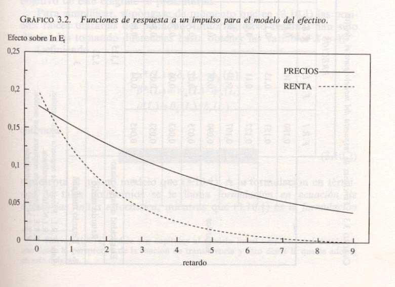
144 4.6 The impact and long-term multipliers

145 IMPACT MULTIPLIERS The impact muliplier of v j shows the change in the dependent variable for a transitional unit change in the exogenous variables j periods before. If the model is in logarithm form, the multipliers are the elasticities.

146 ANALYSIS OF MULTIPLIERS Impact multipliers X jt * = w s (L)/d j (L) X jt = (v 0,j + v 1,j L + v 2,j L 2 + ) X jt where v i,j approximates to zero when i goes to infinity v 0,j, v 1,j, v 2,j are the impact multipliers The impact mulipliers completely characterize the dynamic relation between X j and Y

147 Example X j is a variable in permanent equilibrium, except in the time t = t* X jte, if t<t* X jt = X e jt + 1, if t=t* X jte, if t>t* The dynamics applied to 2L L 4 +L 5 /(1-0.8L) t*

148 IMPACT MULTIPLIERS OF (2) Before t*, the system is in equilibrium, because N t = N e = 0 X t = X e Y t = v(l) X t + N t = v(l)x e + 0 = Y e Y t*-1 = v(l)x t*-1 = v 0 X t*-1 + v 1 X t*-2 + v 2 X t*-3 + = v o X e + v 1 X e + = v(l) X e = Y e Y t* = v(l)x t* = v 0 X t* + v 1 X t*-1 + v 2 X t*-2 + = v o (X e +1) + v 1 X e + = v(l) X e = Y e + v 0 Y t*+1 = v(l)x t*+1 = v 0 X t*+1 + v 1 X t* + v 2 X t*-1 + = v o (X e ) + v 1 (X e +1) + = v(l) X e = Y e + v 1 Y t*+k = v(l)x t*+k = Y e + v k

149 EFFECT OF FILTER ON THE EXPLANATORY VARIABLE X jt * = w s (L)/d j (L) L b X jt = (v 0,j + v 1,j L + v 2,j L 2 + ) X jt L b is lag operator at b periods. w s (L) prolongs the unstructural impulse response during s+1 periods. d r (L) prolongs the response by imposing a certain pattern depending on the roots of the polynomial. Example: impact multipliers associated to 2L L 4 +L 5 /(1-0.8L) v o = v 1 = v 2 = 0 v 6 = 0.8 v 3 = 2 v 7 = v 4 = 2.5 v 8 = v 5 = 1.

150 Because of the stationarity restriction of the polynomial w s (L)/d j (L) L b, the coefficients v j will go to zero as i increases. As mentioned above, Y t*+k = v(l)x t*+k = Y e + v k Implication: the effect of time impact on explanatory variable will disappear by time and Y will go to its equilibrium value Y e.

151 ACCUMULATED MULTIPLIERS The accumulated multiplier V j explains the accumulated change in the dependent variable during (j+1) for a transitional unit change in the explanatory variable j periods before. If the model is in logarithm form, the accumulative multipliers are the elasticities.

152 ACCUMULATED MULTIPLIERS: Before t*, the system is in equilibrium, because N t = N e = 0 X t = X e Y t = v(l) X t + N t = v(l)x e + 0 = Y e But after t*, X e changes permanently to X e +1 Y t*-1 = v(l)x t*-1 = v 0 X t*-1 + v 1 X t*-2 + v 2 X t*-3 + = v o X e + v 1 X e + = v(l) X e = Y e Y t* = v(l)x t* = v 0 X t* + v 1 X t*-1 + v 2 X t*-2 + = v o (X e +1) + v 1 X e + = v(l) X e = Y e + v 0 Y t*+1 = v(l)x t*+1 = v 0 X t*+1 + v 1 X t* + v 2 X t*-1 + = v o (X e +1) + v 1 (X e +1) + = v(l) X e = Y e + v o +v 1 Y t*+k = v(l)x t*+k = Y e + (v 0 + v v k )

153 ACCUMULATED MULTIPLIERS: V 0 = v 0 V 1 = v 0 + v 1 V 2 = v 0 + v 1 + v 2 V k = v 0 + v 1 + v 2 + +v k If v i approaches zero as i increases, V i goes to a constant Vj Constant This constant is the long term multiplier of the filter or the filter gain

154 LONG-TERM MULTIPLIER OR THE GAIN Explains the accumulated change in an infinite horizon in the dependent variable for a transitional unit change in the explanatory variable. If the model is in logarithm, the gain is the long term elasticity.

155 Example Accumulated Multiplier applied to 2L L 4 +L 5 /(1-0.8L) V o = V 1 = V 2 = 0 V 6 = 0.8 V 3 = 2 V 7 = V 4 = 2.5 V 8 = V 5 = 1. Long term multiplier: = 9.5

156 CALCULATING THE LONG RUN MULTIPLIER Given the filter: w s (L)/d j (L) g = (w 0 + w 1 + w w s )/(1-d 1 -d 2 - -d r )

157 4.7. Examples of single-equation dynamic models.

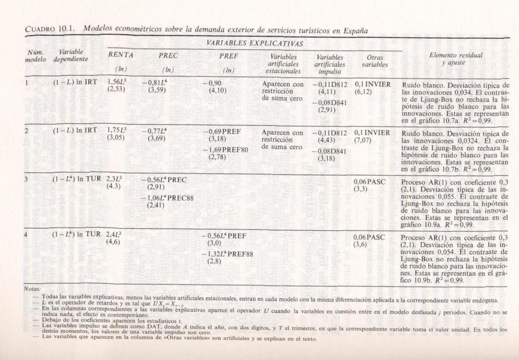
158 MODEL OF TOURISM DEMAND IN SPANISH ECONOMY Read Espasa y Cancelo(eds.),1993, chapter 10.

159 EXAMPLE OF MODEL WITH DIFFERENCE VARIABLES: THE TOURISM DEMAND IN SPAIN Chapter 10 of Espasa and Cancelo (1993), models were built for the tourism demand of foreigners in Spain. The endogeneous variables are income of corresponding types of tourism in constant pesetas.

160 The explanatory variables are: (1) a real income index for tourists (2) an index of relative price in Spain with respect to the client countries and (3) an index of relative price with respect to other destination countries. In this case, all the explanatory variables are exogenous.

161 Model of tourism demand in Spain In the previous slide, there omitted a very important variable for tourism demand, it is the improvement Spain's tourism offer. There is not any observation of this variable and its effect is hidden in the residual term. The omited variable is not stationary oscillations at local level, that means with a unit root, the residuals is not stationary with a difference in its autoregresive part.

162 Model of the tourism demand in Spain Besides, in the data set there are no variables which explain the seasonal habits of the tourists, so the seasonal evolutionarity of the endogenous variable is also hidden in the residual term. The difference (in the residual term) will also be seasonal.

163

164 ESTIMATION AND INTERPRETATION FOR MODEL OF TOURISM RETURN As above, the model will estimate all variables in annual differences whose residuals are stationary. For the purpose of interpretation, it is advisable to use the variables in the model with different levels from the difference operator to the denominator of residuals. This formulation shows that a part of the trend and stationarity of the tourism revenues will not be explained by the economic variables in the model.

165 In the previous example, it is noticed that the tourism revenues, the I(2) variable, represents the systematic growth, and its univariate model requires 2 differentiations, regular and seasonal ones. The previous econometric model shows that the revenue index that is I(2) explanatory variable, has an important contribution to explain tourism trend. It is the factor of the model which explains the growth trend.

166 ADDITIONAL MATERIALS

167 SUMMARY ABOUT SINGLE EQUATION MODELS Generally, in a firm, it is important to combine a variable of interest with other related variables.

168 - This implies using a multivariate data set consisting of observations of the variable of interest and other related variables - This implies working with a multiequation econometric model, for example, a VAR(p) model.

169 A VAR(2) model with two variables will have the following form. X 1t = 11 (1) X 1t (1) X 2t (2) X 1t (2) X 2t-2 + a 1t (4a) X 2t = 21 (1) X 1t (1) X 2t (2) X 1t (2) X 2t-2 + a 2t (4b) Residual variance: Var(a t )

170 -In these models, the variable of interest is determined by other variables and those, in turn, are determined by the variable of interest. In that case, there is a feedback or the Granger causality between each pair of variables, the vector is bidirectional. Watch slide 55 and its followings.

171 - In certain problems, it may be reasonable to think that the causality between the variable of interest and the others is unidirectional way from the latter to the former. - In this case, it is possible to analyze the variable of interest using the single equation model containing that variable and the others. x

172 -If a VAR model is recursive, we can take any equation and analyze it individually. - A VAR model is recursive when: and (a) it has a triangular dynamic structure (b) the residual variance and covariance matrix is diagonal. In this case, all the regressors of any equation are exogenous variables. x

173 -When condition (a) is satisfied whereas condition (b) is not, it is possible to ortogonalize the residuals to obtain a VAR model with conditions (a) and (b) with which we can form an equation relating to the variable of interest. It will be determined specifically by the contemporary values of the explanatory variables, which have become exogenous variables in the reformed VAR model thanks to the ortogonalization. Go to slide 83 and its following slides x

174 -So, in a single equation dynamic model, the present value of the variable of interest (endogenous one) is determined by its past values and the present and past values of other variables. x

175 -The single equation dynamic model can be formulated in terms of Autoregressive Distributed Lag (ADL) or Transfer Function (FT) -Using a sufficient number of lags, both formulations are practically indifferent, once the model is estimated. For the purpose of estimation, one formulation may be more preferable than the other. ADL is often used. x

176 -When the variables are integrated, the model in levels may have stationary residuals, in that case it is said that the variables are cointegrated. x

177 -A single equation model between 2 cointegrated variables will be formulated by the error correction mechanism, so: - (a) generally the formulation is made upon the parameters of interest and, - (b) this is the recommended way to make statistical inference. x

178 If in a single equation model, the variable of interest is not cointegrated with the others, the residuals will not be stationary and the model must be formulated upon differentiated variables. In these cases, the estimation of a model in levels may be spurious x

179 EXAMPLE ON TRANSFER FUNCTION MODEL. Cement consumption in the Spanish economy CEM = Cement consumption RES = Residence NRES = No residence OC = Civil Works All variables are in logs and their first differences. CEM t = (0.12 L L 3 ) RES t + ( L 3 ) NRES t OC t + (1-0.32L)/(1+0.83L 2 ) a t

180 In the above example of the cement consumption in the Spanish economy (CEM) depends on: - RES: production in residential building - NRES: production in non-residential building - OC: production in civil construction. Among the three variables, the denominators of polynomial ratios are unity.

181 THE STRUCTURE OF A SINGLE EQUATION DYNAMIC MODEL The econometric model is an identity, therefore: The features present in the endogenous variable on the left hand side of the equation must be explained by the terms in the right hand side. The terms on the right hand side of the equation are: (a) The exogenous variables (b) The dynamic polynomial ratios for each variable (c) The dynamic polynomials of residuals (d) Innovations

182 ADL and FT MODELS The general structure of FT model is y t k j1 w d j j (L) (L) x The dynamic relationship between y t and each explanatory variable x jt is collected by a polynomial ratio: w j (L) / δ j (L), (L) (L) Additionally, the omitted variables may have a dynamic effect on y t and is collected in a residual term: jt a t. (2) N t (L) (L) a t.

183 ALTERNATIVE FORMULATIONS OF DYNAMIC REGRESSION MODEL Rational distributed lag models or transfer function models (FT). General form: Y t = S j=1 m (w o,j + w 1,j L + + w s,j L s,j ) X jt + q (L) a t (1-d 1j L - - d rj L rj ) p+q (L ) Dynamic effect of the variables Dynamic residual Explantory variables

184 FT MODELS The general structure is y t k w (L) j (L) x a. jt t j 1 d (L) (L) (2) j The dynamic relation between y t and each explanatory variable x jt is collected by a polynomial ratio: w j (L) / δ j (L), Additionally, the omitted variables may have a dynamic effect on y t and is collected in a residual term: N t (L) (L) a t.

185 THE RESIDUAL TERM IN FT MODEL Ф(L)N t = θ(l)a t N t = Ф 1 N t Ф p N t-p - θ 1 a t θ q a t-q + a t N t Nˆ t a t where Nˆ t collects all the dependence of residual term in the past. It is the predictable residual term.

186 FT MODEL Economic theory requires information about the vector of variables that appear in the model and some guidance on the type of dynamic structures between exogenous and endogenous variables.

187 RESPONSE FUNCTION WITH RESPECT TO THE CHANGE IN AN EXPLANATORY VARIABLE X j The general dynamic relationship between X j and Y can be represented by a polynomial of the form: v,j (L) = v 0,j + v 1,j L + v 2,j L The response may be of order, but it must be convergent, so it can be approximated by the ratio of finite order polynomials of the form w s,j (L)/d r,j (L), that was shown in the previous slide. Implication: the reality. the effect of a transitional variable of X j on Y is not permanent. This seems to be a feature of

188 EXAMPLE X j is a variable in long run equilibrium, except the time t = t* X jte, if t < t* X jt = X e jt + 1, if t = t* X jte, if t > t* Dynamic state associated to 2L L 4 +L 5 /(1-0.8L) t*

189 THE SINGLE DYNAMIC LINEAR MODEL a t innovation q (L)/ p+q (L) N t Y t Dependent variable X jt Exogeneous variable w sj (L)/d rj (L) X jt *

190 Ŷ t X jt * Contribution of the explanatory variables (the part of Y explained by the values of X j s). The filter has to be stationary. Nˆ What is predictable in the residual term. Due mainly to the effect of omitted variables. It is not necessary to assume stationarity t

191 MODEL WITH DIFERENCED VARIABLES If the non-stationarity of the endogenous variable is not fully explained by the non-stationarity of the exogenous variables, the residual term is not stationary with unit roots in autoregressive part, ie, the denominator of polynomial structure in which difference operators appear to correspond to unit roots. Multiplying both sides of the model by these operators, they disappear from the residual term and all variables in the model, endogenous and exogenous ones, were differentiated.

192 TRANSFER FUNCTION MODEL: EFECTIVE DEMAND IN SPANISH ECONOMY Véase Espasa and Cancelo (eds.), 1993, pgs 211 to 214.

193

194