Linear Regression with Time Series Data
|
|
|
- Joshua Russell
- 5 years ago
- Views:
Transcription
1 u n i v e r s i t y o f c o p e n h a g e n d e p a r t m e n t o f e c o n o m i c s Econometrics II Linear Regression with Time Series Data Morten Nyboe Tabor
2 u n i v e r s i t y o f c o p e n h a g e n d e p a r t m e n t o f e c o n o m i c s Learning Goals Give an interpretation of the linear regression model for stationary time series and explain the model s identifying assumptions. Derive the method of moments (MM) estimator and state the assumptions used to derive the estimator. Estimate and interpret the parameters. Explain the sufficient conditions for consistency, unbiasedness, and asymptotic normality of the method of moments estimator in the linear regression model. Construct misspecification tests and analyze to what extent a statistical model is congruent with the data. Explain the consequences of autocorrelated, heteroskedastic, and non-normal residuals for the properties of the MM estimator. Econometrics II Linear Regression with Time Series Data Slide 2/47
3 u n i v e r s i t y o f c o p e n h a g e n d e p a r t m e n t o f e c o n o m i c s Outline 1 The Linear Regression Model Definition, Interpretation, and Identification 2 How do we identify and interpret parameters of the model? Method of Moments (MM) Estimation 3 Properties of the Estimator Consistency Unbiasedness Example: Bias in AR(1) Model Asymptotic Distribution 4 Dynamic Completeness and Autocorrelation A Dynamically Complete Model Autocorrelation of the Error Term Consequences of Autocorrelation 5 Model Formulation and Misspecification Testing Model Formulation Misspecification Testing Model Formulation and Misspecification Testing in Practice 6 The Frisch-Waugh-Lovell Theorem 7 Recap: Linear Regression Model with Time Series Data Econometrics II Linear Regression with Time Series Data Slide 3/47
4 1. The Linear Regression Model


 model: y t = θ 1 y t 1 + x t ϕ 0 + x t 1 ϕ 1 + ɛ t.")
5 u n i v e r s i t y o f c o p e n h a g e n d e p a r t m e n t o f e c o n o m i c s Time Series Regression Models Consider the linear regression model y t = x t β + ɛ t = x 1tβ 1 + x 2tβ x kt β k + ɛ t, for t = 1, 2,..., T. Note that y t and ɛ t are 1 1, while x t and β are k 1. The interpretation of the model depends on the variables in x t. 1 If x t contains contemporaneously dated variables, it is denoted a static regression: y t = x t β + ɛt. 2 A simple model for y t given the past is an autoregressive model: y t = θy t 1 + ɛ t. 3 More complicated dynamics in the autoregressive distributed lag (ADL) model: y t = θ 1 y t 1 + x t ϕ 0 + x t 1 ϕ 1 + ɛ t. Econometrics II Linear Regression with Time Series Data Slide 5/47
6 2. How do we identify and interpret parameters of the model?
 E(ɛ t) = 0. (B) E(ɛ t x t) = 0. (C) E(ɛ t x 1t, x 2t,..., x t,..., x T ) = 0. (D) E(x tɛ t) = 0. (E) Don t know. Please go to www.socrative.")
7 Socrative Question 1 Consider the linear regression model for time series, y t = x t β + ɛ t, t = 1, 2,..., T. ( ) Q: Which one of the following assumptions identifies the parameters β in ( )? (A) E(ɛ t) = 0. (B) E(ɛ t x t) = 0. (C) E(ɛ t x 1t, x 2t,..., x t,..., x T ) = 0. (D) E(x tɛ t) = 0. (E) Don t know. Please go to click Student login, and enter room id Econometrics2.
 As it stands, the equation is a tautology: not informative on β! Why?... For any β, we can find a residual ɛ t so that ( ) holds.")
 represents the conditional expectation, E(y t x t) = x t β, so that E (ɛ t x t) = 0. ( ) This condition states a zero-conditional-mean. We say that x t is predetermined.")
8 u n i v e r s i t y o f c o p e n h a g e n d e p a r t m e n t o f e c o n o m i c s Interpretation of Regression Models Consider again the regression model y t = x t β + ɛ t, t = 1, 2,..., T. ( ) As it stands, the equation is a tautology: not informative on β! Why?... For any β, we can find a residual ɛ t so that ( ) holds. We have to impose restrictions on ɛ t to ensure a unique solution to ( ). This is called identification in econometrics. Assume that ( ) represents the conditional expectation, E(y t x t) = x t β, so that E (ɛ t x t) = 0. ( ) This condition states a zero-conditional-mean. We say that x t is predetermined. Under assumption ( ) the coefficients are the partial (ceteris paribus) effects E(y t x t) x jt = β j. Econometrics II Linear Regression with Time Series Data Slide 7/47
 E(ɛ t) = 0. (B) E(ɛ t x 1t, x 2t,..., x t,..., x T ) = 0. (C) E(x tɛ t) = 0. (D) E(xt 2 ɛ t) = 0.")
9 Socrative Question 2 Consider the linear regression model for time series, y t = x t β + ɛ t, t = 1, 2,..., T, ( ) where we assume the regressors are predetermined, E(ɛ t x t) = 0. Q: Which of the following assumptions is not implied by predeterminedness? (A) E(ɛ t) = 0. (B) E(ɛ t x 1t, x 2t,..., x t,..., x T ) = 0. (C) E(x tɛ t) = 0. (D) E(xt 2 ɛ t) = 0. (E) Don t know.
10
11 u n i v e r s i t y o f c o p e n h a g e n d e p a r t m e n t o f e c o n o m i c s Identification Predeterminedness implies the so-called moment condition: stating that x t and ɛ t are uncorrelated. E (x tɛ t) = 0, ( ) Now insert the model definition, ɛ t = y t x t β, in ( ) to obtain E(x t(y t x t β)) = 0 E(x ty t) E(x tx t )β = 0. This is a system of k equations in the k unknown parameters, β, and if E(x tx t ) is non-singular we can find the so-called population estimator which is unique. β = E(x tx t ) 1 E(x ty t), The parameters in β are identified by ( ) and the non-singularity condition. The latter is the well-known condition for no perfect multicollinearity. Econometrics II Linear Regression with Time Series Data Slide 8/47
12 u n i v e r s i t y o f c o p e n h a g e n d e p a r t m e n t o f e c o n o m i c s Method of Moments (MM) Estimation From a given sample (y t, x t ), t = 1, 2,..., T, we cannot compute expectations. In practice we replace with sample averages and obtain the MM estimator ( ) 1 ( ) T T β = T 1 x tx t T 1 x ty t. t=1 Note that the MM estimator coincides with the OLS estimator. For MM to work, i.e., β β, we need a law of large numbers (LLN) to apply, i.e., T 1 T x ty t E(x ty t) and T 1 t=1 t=1 T x tx t E(x tx t ). Note the two distinct conditions for OLS to converge to the true value: t=1 1 The moment condition ( ) should be satisfied. 2 A law of large numbers should apply. A central part of econometric analysis is to ensure these conditions. Econometrics II Linear Regression with Time Series Data Slide 9/47

. (A) True. (B) False. (C). (D).")
13 Socrative Question 3 Consider the linear regression model for time series, y t = x t β + ɛ t, for t = 1, 2,..., T. Q: Is the following statement true or false? We can only calculate the method of moments (MM) estimator, β, if the time series y t and x t are stationary (and weakly dependent). (A) True. (B) False. (C). (D). (E) Don t know.

14
15
16 u n i v e r s i t y o f c o p e n h a g e n d e p a r t m e n t o f e c o n o m i c s Main Assumption We impose assumptions to ensure that a LLN applies to the sample averages. Main Assumption Consider a time series y t and the k 1 vector time series x t. We assume: 1 The process z t = (y t, x t ) has a joint stationary distribution. 2 The process z t is weakly dependent, so that z t and z t+h becomes approximately independent for h. Interpretation: Think of (1) as replacing identical distributions for IID data. Think of (2) as replacing independent observations for IID data. Under the main assumption, most of the results for linear regression on random samples carry over to the time series case. Econometrics II Linear Regression with Time Series Data Slide 10/47
17 Matrix Notation
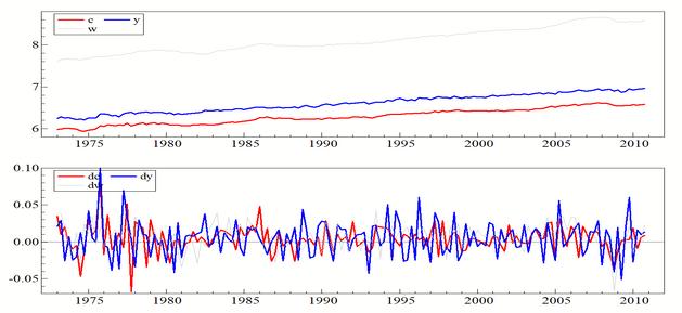
18 Empirical Example: Consumption, Income, and Wealth Say that we want to estimate the effect of households income and wealth on consumption. We have quarterly Danish data from 1973(1) to 2010(4). Where do we start?
19 1. Graphs
20 3. Properties of the Estimator
21 Monte Carlo Illustration: Static Regression 1 We simulate M replications from the data generating process, y t = b 1z 1t + e t, t = 1, 2,..., T, (1) where z 1t N(0, 1), e t N(0, 1), and b 1 = 1. 2 For each replication of (y t, z 1t), we estimate the static linear regression model by OLS, which gives the estimates β(m) T size T. We plot, The distributions of β(m) M 1 M (MCSD). m=1 β (m) T y t = β 0 + β 1z 1t + ɛ t, t = 1, 2,..., T, (2) T. for m = 1, 2,..., M and given the sample plus-minus two Monte Carlo standard deviations for an increasing sample size T {20, 30,..., 1000}. What do you see?


22 Simulation Settings in OxMetrics We run the simulations in OxMetrics. Choose Model, select the PcGive module with the category Monte Carlo and model class Static Experiment using PcNaive. We use the settings:
23 What Do You See? Za Constant Za 2MCSD 0.50 Constant 2MCSD
24 The Linear Regression Model and the MM Estimator
25
26 Socrative Question 4 Consider the linear regression model, y t = x t β + ɛ t, for t = 1, 2,..., T, where we assume that x t is a single explanatory with E(x t) = 0. The MM estimator can be written as β = T t=1 xtyt T t=1 x 2 t = β + T t=1 xtɛt T t=1 x 2 t. Q: In addition to stationarity, what is required for consistency of the MM estimator, β β for T? (A) Strict exogeneity: E(ɛ t x 1, x 2,..., x T ) = 0. (B) Predeterminedness: E(ɛ t x t) = 0. (C) Moment conditions: E(x tɛ t) = 0. (D) Conditional homoskedasticity and no serial correlation: E(ɛ 2 t x t) = σ 2 and E(ɛ tɛ s x t, x s) = 0. (E) Don t know. Please go to click Student login, and enter room id Econometrics2.
27
28 u n i v e r s i t y o f c o p e n h a g e n d e p a r t m e n t o f e c o n o m i c s Consistency Consistency is the first requirement for an estimator: β should converge to β. Result 1: Consistency Let y t and x t obey the main assumption. If the regressors obey the moment condition, E(x tɛ t) = 0, then the OLS estimator is consistent, i.e., β β as T. The OLS estimator is consistent if the regression represents the conditional expectation of y t x t. In this case E(ɛ t x t) = 0, and β i has a ceteris paribus interpretation. The conditions in Result 1 are sufficient but not necessary. We will see examples of estimators that are consistent even if the conditions are not satisfied (related to unit roots and cointegration). Econometrics II Linear Regression with Time Series Data Slide 12/47
29 u n i v e r s i t y o f c o p e n h a g e n d e p a r t m e n t o f e c o n o m i c s Illustration of Consistency Consider the regression model with a single explanatory variable, k = 1, y t = x tβ + ɛ t, t = 1, 2,..., T, with E (x tɛ t) = 0 and E(x t) = 0. Write the OLS estimator as β = T 1 T t=1 ytxt T 1 T t=1 x 2 t = T 1 T (xtβ + ɛt)xt t=1 T 1 T x 2 t=1 t = β + T 1 T t=1 ɛtxt T 1 T t=1 x 2 t and look at the terms as T : T plim T 1 T xt 2 = σx, 2 0 < σx 2 < ( ) plim T 1 T t=1 T ɛ tx t = E (ɛ tx t) = 0 t=1 Where LLN applies under Assumption 1; and ( ) holds for a stationary process (σ 2 x is the limiting variance of x t). ( ) follows from predeterminedness., ( ) Econometrics II Linear Regression with Time Series Data Slide 13/47
30 Proof of Unbiasedness The MM estimator in the linear regression model for stationary time series can be written as Assuming strict exogeneity, T t=1 β = β + xtɛt T. t=1 xtx t E(ɛ t x 1, x 2,..., x T ) = 0, the MM estimator is conditionally and unconditionally unbiased. 1 Use the law of iterated expecations to prove that the assumption of strict exogeneity implies that the MM estimator is conditionally unbiased: E(ɛ t x 1, x 2,..., x T ) = 0 E( β x1, x 2,..., x T ) = 0. 2 Use the law of iterated expectations to prove that conditional unbiasedness implies unconditional unbiasedness: E( β x1, x 2,..., x T ) = 0 E( β) = 0
 = 0, then the OLS estimator is unbiased, i.e., E( β x1, x 2,.")
31 u n i v e r s i t y o f c o p e n h a g e n d e p a r t m e n t o f e c o n o m i c s Unbiasedness A stronger requirement for an estimator is unbiasedness: E( β) = β. Result 2: Unbiasedness Let y t and x t obey the main assumption. If the regressors are strictly exogenous, E (ɛ t x 1, x 2,..., x t,..., x T ) = 0, then the OLS estimator is unbiased, i.e., E( β x1, x 2,..., x T ) = β. Econometrics II Linear Regression with Time Series Data Slide 14/47
32 u n i v e r s i t y o f c o p e n h a g e n d e p a r t m e n t o f e c o n o m i c s Unbiasedness A stronger requirement for an estimator is unbiasedness: E( β) = β. Result 2: Unbiasedness Let y t and x t obey the main assumption. If the regressors are strictly exogenous, E (ɛ t x 1, x 2,..., x t,..., x T ) = 0, then the OLS estimator is unbiased, i.e., E( β x1, x 2,..., x T ) = β. Unbiasedness requires strict exogeneity, which is not fulfilled in a dynamic regression. Consider the first order autoregressive model y t = θy t 1 + ɛ t. Here y t is function of ɛ t, so ɛ t cannot be uncorrelated with y t, y t+1,..., y T. Result 3: Estimation bias in dynamic models In general, the OLS estimator is not unbiased in regressions with lagged dependent variables. Econometrics II Linear Regression with Time Series Data Slide 14/47
33 u n i v e r s i t y o f c o p e n h a g e n d e p a r t m e n t o f e c o n o m i c s Example: Finite Sample Bias in an AR(1) Consider a first-order autoregressive, AR(1), model, y t = θy t 1 + ɛ t, t = 1, 2,..., T, ( ) where θ = 0.9. The time series y t satisfy Assumption 1 of stationarity and weak dependence (we will return to the properties of y t later). The OLS estimator is, ( T ) 1 ( T θ = t=1 y 2 t 1 t=1 y t 1y t ) We are often interested in E( θ) to check for bias for a given T. This is typically difficult to derive analytically.. But if we could draw realizations of θ, then we could estimate E( θ). Econometrics II Linear Regression with Time Series Data Slide 15/47
34 u n i v e r s i t y o f c o p e n h a g e n d e p a r t m e n t o f e c o n o m i c s Finite Sample Bias in an AR(1) MC simulation: 1 Construct (randomly) M artificial data sets from the AR(1) model ( ). 2 Estimate the model ( ) for each data set and get the estimates, θ(m), for m = 1, 2,..., M. 3 Compute the Monte Carlo mean, the Monte Carlo standard deviation, and an estimate of the bias: M MEAN( θ) = M 1 θ (m) MCSD( θ) = m=1 M ( θ(m) ) 2 M 1 MEAN( θ) m=1 Bias( θ) = MEAN( θ) θ. Note that by the LLN (for independent observations, since the θ(m) s are independent): M MEAN( θ) = M 1 θ (m) E( θ) for M. m=1 Econometrics II Linear Regression with Time Series Data Slide 16/47
35 u n i v e r s i t y o f c o p e n h a g e n d e p a r t m e n t o f e c o n o m i c s Finite Sample Bias in an AR(1): Monte Carlo Simulations in PcNaive We consider Monte Carlo simulations to illustrate potential bias of the OLS estimator for θ in the AR(1) model, ( ). We consider the parameter values: θ {0.0, 0.5, 0.9}. This can be done quite easily in the module PcNaive in OxMetrics. 1 In OxMetrics, click the Model menu and select Model. 2 In the window that pops up, select the PcGive module. In Category select Monte Carlo and in Model class select AR(1) Experiment using PcNaive. 3 Click Formulate. 4 In the Formulate window you must specify the DGP, the estimating model, the number of replications, the sample length(s), and some output settings. See next slide. Econometrics II Linear Regression with Time Series Data Slide 17/47
: PcNaive Econometrics II Linear Regression with Time Series Data Slide")
36 u n i v e r s i t y o f c o p e n h a g e n d e p a r t m e n t o f e c o n o m i c s Finite Sample Bias in an AR(1): PcNaive Econometrics II Linear Regression with Time Series Data Slide 18/47
37 u n i v e r s i t y o f c o p e n h a g e n d e p a r t m e n t o f e c o n o m i c s Finite Sample Bias in an AR(1): PcNaive Output for θ = 0 Ya_ Ya_1 2MCSD Econometrics II Linear Regression with Time Series Data Slide 19/47
38 u n i v e r s i t y o f c o p e n h a g e n d e p a r t m e n t o f e c o n o m i c s Finite Sample Bias in an AR(1): PcNaive Output for θ = 0.5 Ya_ Ya_1 2MCSD Econometrics II Linear Regression with Time Series Data Slide 20/47
39 u n i v e r s i t y o f c o p e n h a g e n d e p a r t m e n t o f e c o n o m i c s Finite Sample Bias in an AR(1): PcNaive Output for θ = Ya_ Ya_1 2MCSD Econometrics II Linear Regression with Time Series Data Slide 21/47
40 u n i v e r s i t y o f c o p e n h a g e n d e p a r t m e n t o f e c o n o m i c s Finite Sample Bias in an AR(1) Finite Sample Bias in an AR(1) In a Monte Carlo simulation, we take an AR(1) as the DGP and In a MC simulation we take an AR(1) as the DGP and estimation model: estimation model: = (0 1) y t = 0.9 y t 1 + ɛ t, ɛ t N(0, 1). Mean of OLS estimate in AR(1) model True value MEAN MEAN ± 2 MCSD of 21 Econometrics II Linear Regression with Time Series Data Slide 22/47
 = 0.")
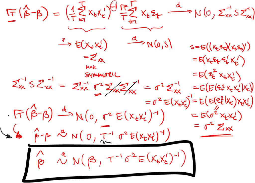
41 u n i v e r s i t y o f c o p e n h a g e n d e p a r t m e n t o f e c o n o m i c s Asymptotic Distribution To derive the asymptotic distribution we need a CLT; additional restrictions on ɛ t. Result 4: Asymptotic distribution and OLS variance Let y t and x t obey the main assumption and let x t and ɛ t be uncorrelated, E(ɛ tx t) = 0. Furthermore, assume (conditional) homoskedasticity and no serial correlation, i.e., E ( ) ɛ 2 t x t = σ 2 E (ɛ tɛ s x t, x s) = 0 for all t s. Then as T, the OLS estimator is asymptotically normal with usual variance: T ( β β ) D N(0, σ 2 E(x tx t ) 1 ). Inserting estimators, we can test hypotheses using ( ( T ) 1 ) β a N β, σ 2 x tx t. t=1 Recall that E(ɛ tx t) = 0 is implied by E[ɛ t x t] = 0. Econometrics II Linear Regression with Time Series Data Slide 23/47
42
43 Empirical Example: The Linear Regression Model
44 Empirial Example: Estimates
45 4. Dynamic Completeness and Autocorrelation
46 u n i v e r s i t y o f c o p e n h a g e n d e p a r t m e n t o f e c o n o m i c s A Dynamically Complete Model Result 4 (Asymptotic distribution of the OLS estimator) required no serial correlation in the error terms. The precise condition for no serial correlation looks strange. Often we disregard conditioning and consider whether ɛ t and ɛ s are uncorrelated. We say that a model is dynamically complete if E(y t x t, y t 1, x t 1, y t 2, x t 2,..., y 1, x 1) = E(y t x t) = x t β. x t contains all relevant information in the available information set. No-serial-correlation is practically the same as dynamic completeness. All systematic information in the past of y t and x t is used in the regression model. This is often taken as an important design criteria for a dynamic regression model. We should always test for no-autocorrelation in time series models. Econometrics II Linear Regression with Time Series Data Slide 25/47
47 u n i v e r s i t y o f c o p e n h a g e n d e p a r t m e n t o f e c o n o m i c s Autocorrelation of the Error Term If Cov(ɛ t, ɛ s) 0 for some t s, we have autocorrelation of the error term. This is detected from the estimated residuals and Cov( ɛ t, ɛ s) 0 is referred to as residual autocorrelation. Often used synonymously. Residual autocorrelation does not imply that the DGP has autocorrelated errors. Typically, autocorrelation is taken as a signal of misspecification. Different possibilities: 1 Autoregressive errors in the DGP. 2 Dynamic misspecification. 3 Omitted variables and non-modelled structural shifts. 4 Misspecified functional form The solution to the problem depends on the interpretation. Econometrics II Linear Regression with Time Series Data Slide 26/47
 = 0 is violated if the model includes a lagged dependent variable. Look at an AR(1) model with error autocorrelation, i.e., the two equations y t = θy t 1 + ɛ t ɛ t = ρɛ t 1 + v t, v t IID(0, σ 2 v ).")
48 u n i v e r s i t y o f c o p e n h a g e n d e p a r t m e n t o f e c o n o m i c s Consequences of Autocorrelation Autocorrelation will not violate the assumptions for Result 1 (consistency) in general. But E(x tɛ t) = 0 is violated if the model includes a lagged dependent variable. Look at an AR(1) model with error autocorrelation, i.e., the two equations y t = θy t 1 + ɛ t ɛ t = ρɛ t 1 + v t, v t IID(0, σ 2 v ). Both y t 1 and ɛ t depend on ɛ t 1, so E(y t 1ɛ t) 0. Result 5: Inconsistency of OLS In a regression model including the lagged dependent variable, the OLS estimator is not consistent in the presence of autocorrelation of the error term. Even if OLS is consistent, the standard formula for the variance in Result 4 is no longer valid. It is possible to derive the variance, the so-called heteroskedasticity-and-autocorrelation-consistent (HAC) standard errors. Econometrics II Linear Regression with Time Series Data Slide 27/47
49
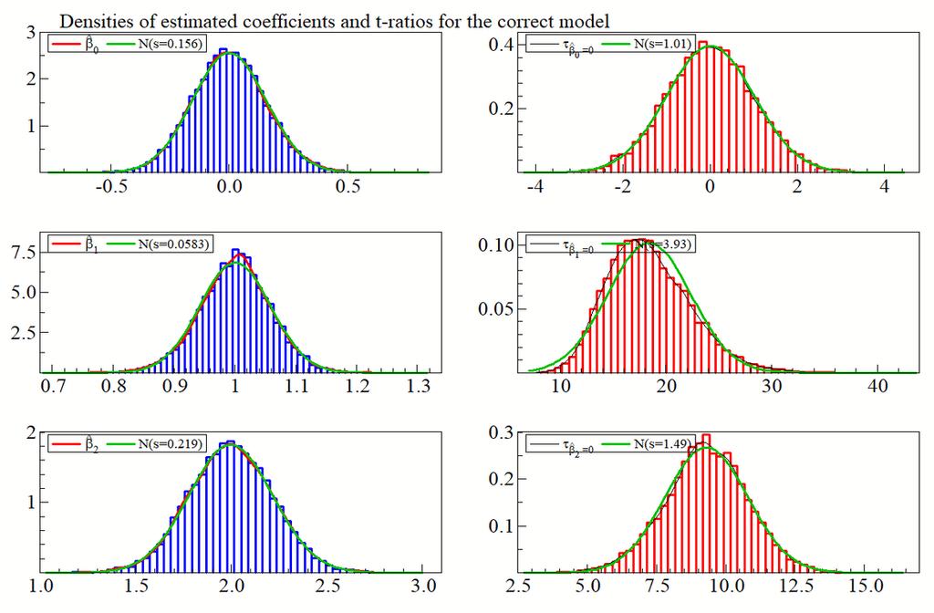
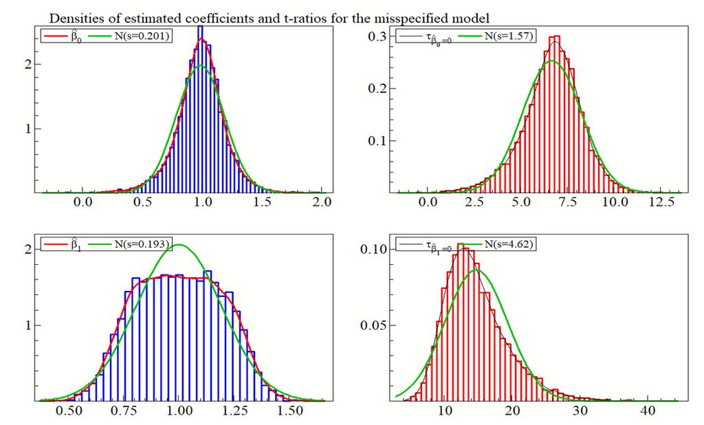
 ( ) for t = 1, 2,..., T, where v t is assumed IIDN(0,1) and the initial values are y 0 = y 1 = 0. We set θ 1 = 0.7, θ 2 = 0.2, and ρ = 0.9.")
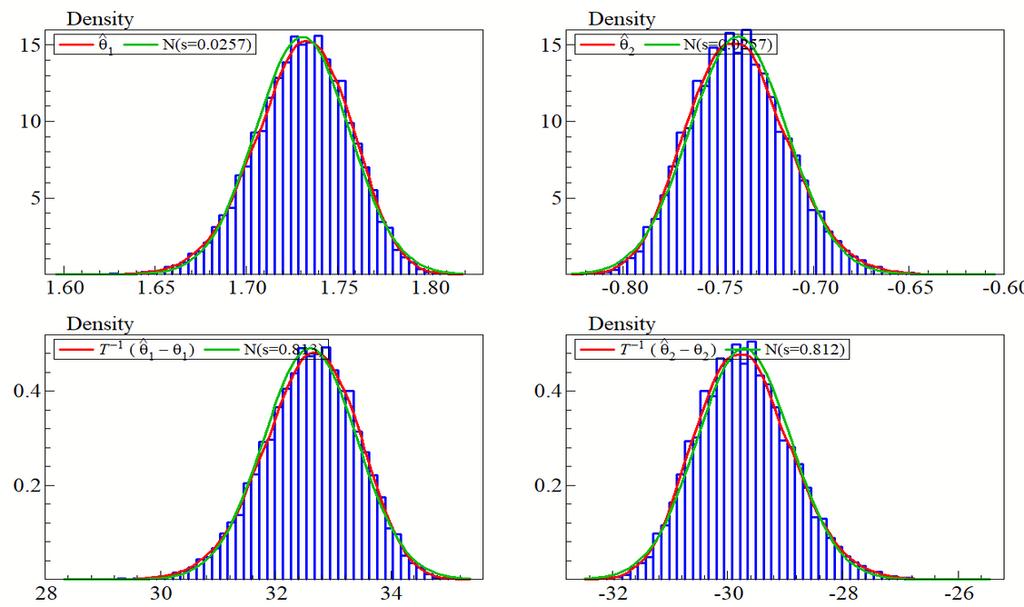
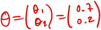
50 Simulation Illustration: Inconsistency in Dynamic Model Data-generating Process We simulate time series from the stationary AR(2) model with autocorrelated errors, y t = θ 1y t 1 + θ 2y t 2 + ɛ t, ɛ t = ρɛ t 1 + v t, ( ) ( ) for t = 1, 2,..., T, where v t is assumed IIDN(0,1) and the initial values are y 0 = y 1 = 0. We set θ 1 = 0.7, θ 2 = 0.2, and ρ = 0.9. We simulate M = 10, 000 replications with sample size T = 200, Estimated Model For the simulated data, we estimate the AR(2) model in ( ) by MM/OLS: ( T ) 1 ( T ) ( θ1 = θ 2 t=1 ( yt 1 y t 2 ) (yt 1 y t 2 ) t=1 ( ) ) yt 1 y y t t 2 We plot the distributions of θ1, θ2, T ( θ1 θ 1), and T ( θ2 θ 2). Consistency of the estimator requires the moment condition, which is violated due to the autocorrelation of the error-term.

51 Simulation Illustration: Inconsistency in Dynamic Model
52
53 Simulation Illustration: Inconsistency in Dynamic Model
54 u n i v e r s i t y o f c o p e n h a g e n d e p a r t m e n t o f e c o n o m i c s (1) Autoregressive Errors in the DGP Consider the case where the errors are truly autoregressive: y t = x t β + ɛ t If ρ is known we can write ɛ t = ρɛ t 1 + v t, v t IID(0, σ 2 v ). (y t ρy t 1) = ( x t ρx t 1) β + (ɛt ρɛ t 1) y t = ρy t 1 + x t β x t 1ρβ + v t. The transformation is analog to GLS transformation in the case of heteroskedasticity. The GLS model is subject to a so-called common factor restriction: three regressors but only two parameters, ρ and β. Estimation is non-linear and can be carried out by maximum likelihood. Econometrics II Linear Regression with Time Series Data Slide 28/47
55 u n i v e r s i t y o f c o p e n h a g e n d e p a r t m e n t o f e c o n o m i c s Consistent estimation of the parameters in the GLS model requires E((x t ρx t 1) (ɛ t ρɛ t 1)) = 0. But then ɛ t 1 should be uncorrelated with x t, i.e., E(ɛ tx t+1) = 0. Consistency of GLS requires stronger assumptions than consistency of OLS. The GLS transformation is rarely used in modern econometrics. 1 Residual autocorrelation does not imply that the error term is autoregressive. There is no a priori reason to believe that the transformation is correct. 2 The requirement for consistency of GLS is strong. Econometrics II Linear Regression with Time Series Data Slide 29/47
56 u n i v e r s i t y o f c o p e n h a g e n d e p a r t m e n t o f e c o n o m i c s (2) Dynamic Misspecification Residual autocorrelation indicates that the model is not dynamically complete, so E(y t x t) E(y t x t, y t 1, x t 1, y t 2, x t 2,..., y 1, x 1). The (dynamic) model is misspecified and should be reformulated. Natural remedy is to extend the list of lags of x t and y t. If autocorrelation seems of order one, then a starting point is the GLS transformation. The AR(1) structure is only indicative and we look at the unrestricted ADL model y t = α 0y t 1 + x t α 1 + x t 1α 2 + η t. Finding of first-order autocorrelation is only used to extend the list of regressors. The common factor restriction is removed. Econometrics II Linear Regression with Time Series Data Slide 30/47
57 u n i v e r s i t y o f c o p e n h a g e n d e p a r t m e n t o f e c o n o m i c s (3) Omitted Variables Omitted variables in general can also produce autocorrelation. Let the DGP be y t = x 1t β 1 + x 2t β 2 + ɛ t, and consider the estimation model ( ) y t = x 1t β 1 + u t. ( ) Then the error term is u t = x 2t β 2 + ɛ t, which is autocorrelated if x 2t is persistent. An example is if the DGP exhibits a level shift, e.g., ( ) includes the dummy variable { 0 for t < T0 x 2t =. 1 for t T 0 If x 2t is not included in ( ) then the residual will be systematic. Again the solution is to extend the list of regressors, x t. Econometrics II Linear Regression with Time Series Data Slide 31/47
58

59
60
61
62 u n i v e r s i t y o f c o p e n h a g e n d e p a r t m e n t o f e c o n o m i c s (4) Misspecified Functional Form If the true relationship y t = g(x t) + ɛ t is non-linear, the residuals from a linear regression will typically be autocorrelated. The solution is to try to reformulate the functional form of the regression line. Econometrics II Linear Regression with Time Series Data Slide 32/47
63 5. Model Formulation and Misspecification Testing
64 u n i v e r s i t y o f c o p e n h a g e n d e p a r t m e n t o f e c o n o m i c s Model Formulation and Properties of the Estimator We consider the linear regression model for time series, y t = x t β + ε t. (*) If there is no perfect multicolleniarity in x t we can always compute the OLS estimator β and consider the estimated model, y t = x t β + ε t, for the sample t = 1, 2,...T. (**) Under specific assumptions can we derive properties of the estimator β: 1 Consistency: β β as T. 2 Unbiasedness: E[ β x1, x 2,..., x T ] = β. 3 Asymptotic distribution: β a N(β, σ 2 ( T t=1 xtx t ) 1 ). However, if ( ) does not satisfy the specific assumptions we cannot use the results in (1)-(3) to interpret the estimated coefficients and to do statistical inference (e.g. test the hypothesis H 0 : β i = 0). Econometrics II Linear Regression with Time Series Data Slide 34/47
65 u n i v e r s i t y o f c o p e n h a g e n d e p a r t m e n t o f e c o n o m i c s Misspecification Testing We can never show that the model is well specified; but we can certainly find out if it is not in a specific direction! Misspecification testing. We consider the following standard tests on the estimated errors, ε t: 1 Test for no-autocorrelation. 2 Test for no-heteroskedasticity. 3 Test for normality of the error term. If all tests are passed, we may think of the model as representing the main features of the data and we can use the results in (1) (3), e.g. for testing hypotheses on estimated parameters. Econometrics II Linear Regression with Time Series Data Slide 35/47
66 u n i v e r s i t y o f c o p e n h a g e n d e p a r t m e n t o f e c o n o m i c s (1) Tests for No-Autocorrelation Let ɛ t (t = 1, 2,..., T ) be the estimated residuals from the original regression model y t = x t β + ɛ t. A test for no-autocorrelation (of first order) is based on the hypothesis γ = 0 in the auxiliary regression ɛ t = x t δ + γ ɛ t 1 + u t, where x t is included because it may be correlated with ɛ t 1. A valid test is t ratio for γ = 0. Alternatively there is the Breusch-Godfrey LM test LM = T R 2 χ 2 (1). Note that x t and ɛ t are orthogonal, and any explanatory power is due to ɛ t 1. The Durbin Watson (DW) test is derived for finite samples. Based on strict exogeneity. Not valid in many models. Econometrics II Linear Regression with Time Series Data Slide 36/47


67 Statistical Testing 1 Null hypothesis: 2 Test statistics: 3 Asymptotic distribution of the test statistics under the null:
68 u n i v e r s i t y o f c o p e n h a g e n d e p a r t m e n t o f e c o n o m i c s (2) Test for No-Heteroskedasticity Consider the auxiliary regression ɛ 2 t = γ 0 + x 1tγ x kt γ k + x 2 1tδ x 2 ktδ k + u t. A test for unconditional homoskedasticity is based on the null hypothesis: γ 1 =... = γ k = δ 1 =... = δ k = 0. The alternative is that the variance of ɛ t depends on x it or the squares x 2 it for some i = 1, 2,...k. The LM test, LM = T R 2 χ 2 (2k). Econometrics II Linear Regression with Time Series Data Slide 37/47
69 u n i v e r s i t y o f c o p e n h a g e n d e p a r t m e n t o f e c o n o m i c s (3) Test for Normality of the Error Term Skewness (S) and kurtosis (K) are the estimated third and fourth central moments of the standardized estimated residuals u t = ( ε t ε)/ σ.: S = T 1 T ut 3 and K = T 1 t=1 T ut 4. The normal distribution is symmetric and has S = 0, while K = 3 (K 3 is often referred to as excess kurtosis). If K > 3, the distribution has fat tails. Under the assumption of normality, t=1 ξ S = T 6 S2 χ 2 (1) ξ K = T 24 (K 3)2 χ 2 (1). It turns out that ξ S and ξ K are independent: Jarque-Bera joint test of normality: ξ JB = ξ S + ξ K χ 2 (2). Econometrics II Linear Regression with Time Series Data Slide 38/47
70 u n i v e r s i t y o f c o p e n h a g e n d e p a r t m e n t o f e c o n o m i c s Notes on Normality of the Error Term Often normality of the error terms is rejected due to the presence of a few large outliers that the model cannot account for (i.e. they are captured by the error term). Start with a plot and a histogram of the (standardized) estimated residuals. Any large outliers of, say, more than three standard deviations? A big residual at time T 0 may be accounted for by including a dummy variable (x t = 1 for t = T 0, x t = 0 for all other t). Note that the results for the linear regression model hold without assuming normality of ε t. However, the normal distribution is a natural benchmark and given normality: β converges faster to the asymptotic normal distribution. The OLS estimator coincides with the maximum likelihood (ML) estimator. Econometrics II Linear Regression with Time Series Data Slide 39/47
71 u n i v e r s i t y o f c o p e n h a g e n d e p a r t m e n t o f e c o n o m i c s Model Formulation and Misspecification Testing in Practice Finding a well-specified model for the data of interest can be hard in practice! Potential reasons include: Which variables to include in x t? Economic theory can often guide us. How many lags to include to obtain a dynamically complete model? Are the model parameters constant over the sample or do we need to include structural breaks? Do we need to include dummy variables to capture large outliers? Think about which model and which formulation is useful to represent the characteristics of the data! In practice we use an iterative procedure: 1 Estimate the model for a specific formulation. 2 Do misspecification tests on the estimated errors. 3 If the misspecification tests are rejected, re-formulate the model. Repeat (1) and (2) until the misspecification tests are not rejected. General-to-Specific: Start with a larger model and simplify it by removing insignificant variables. Econometrics II Linear Regression with Time Series Data Slide 40/47
72 Socrative Question 5 For the estimated model for consumption, we get the following output for the test for no autocorrelation of order 1-2. Error autocorrelation coefficients in auxiliary regression: Coefficient Std.Error t value Lag Lag RSS = sigma = Testing for error autocorrelation from lags 1 to 2 Chi^2(2) = [0.0557] and F form F(2,145) = [0.0592] Q: What is your conclusion to the LM test for no autocorrelation of order 1-2? (A) We cannot reject the null of autocorrelation. (B) We cannot reject the null of no autocorrelation. (C) We reject the null of autocorrelation. (D) We reject the null of no autocorrelation. (E) Don t know. Please go to click Student login, and enter room id Econometrics2.
73
74 Socrative Question 6 Let the Jarque-Berra test for normality of the estimated residuals give the following test statistics, ξ JB = ξ S + ξ K = 4.9. Q: What is your conclusion to the test based on a 5 percent significance level? (A) We cannot reject the null of normality of the estimated residuals. (B) We reject the null of normality of the estimated residuals. (C). (D). (E) Don t know.
75 Socrative Question 7 Q: Which of the following statements is correct if the error term is heteroskedastic? (A) β is inconsistent. (B) β is inconsistent, but T ( β β) is asymptotically normal. (C) β is consistent, but T ( β β) is not asymptotically normal. (D) β is consistent and T ( β β) is asymptotically normal. (E) Don t know.
76
77 Socrative Question 8 Q: Why do we care about normality of the error term? (A) If ɛ t Niid(0, σ 2 ), then the MM estimator converges faster to the asymptotic normal distribution and it is efficient. (B) The MM estimator is inconsistent if ɛ t is not normally distributed and independent over time. (C) The t-test of the null that β i = 0, t βi =0 = βi/s.e.( βi) is only asymptotically N(0, 1) if ɛ t Niid(0, σ 2 ). (D) The MM estimator is not asymptotically normally distributed unless ɛ t is normally distributed. (E) Don t know.
78 Empirical Example: Consumption, Income, and Wealth We consider the model for consumption c t = δ + γ 1 y t + γ 2 w t + αecm t 1 + ɛ t, for t = 1, 2,..., T, where ɛ t is assumed IID(0,σ 2 ) and ECM t 1 is defined as ECM t 1 = c t y t w t 1. We estimate the model by MM/OLS using quarterly data for 1973(1) 2010(4).
79 Empirical Example: Consumption, Income, and Wealth
80 Empirical Example: Consumption, Income, and Wealth Based on the graphs of the estimated residuals, discuss which of the following assumptions are satisfied for the estimated model. Explain how you reach your conclusion. (1) Stationarity of (y t, x t). (2) Predeterminedness: E(ɛ t x t) = 0. Zero-mean: E(ɛ t) = 0. Moment-condition: E(x tɛ t) = 0. (3) Homoskedasticity: E(ɛ 2 t x t) = σ 2 E(ɛ 2 t ) = σ 2. (4) No serial correlation: E(ɛ tɛ s x t, x s) = 0 E(ɛ tɛ t k ) = 0. (5) Normally distributed errors: ɛ t N(0, σ 2 ). Do you notice anything else we should think about?
81 Socrative Question 9 For the estimated model for consumption, we get the misspecification tests: AR 1 5 test: F(5,142) = [0.0891] Normality test: Chi^2(2) = [0.0000]** Hetero test: F(6,144) = [0.0346]* Q. What do you conclude regarding the misspecification tests? (A) The estimated residuals are not autocorrelated, homoskedastic, and normal. (B) The estimated residuals are homoskedastic and normal, but autocorrelated. (C) The estimated residuals are not autocorrelated, but heteroskedastic and non-normal. (D) The estimated residuals are autocorrelated, heteroskedastic, and non-normal. (E) Don t know. Please go to click Student login, and enter room id Econometrics2.
82 6. The Frisch-Waugh-Lovell Theorem
83 u n i v e r s i t y o f c o p e n h a g e n d e p a r t m e n t o f e c o n o m i c s Motivation Consider the linear regression model, y t = µ + β 1x t + ε t, t = 1, 2,..., T, (3) and the linear regression model for the de-meaned variables ỹ t = y t ȳ and x t = x t x, given by Question: Would you expect ˆβ 1 to equal ˆb 1? ỹ t = b 1 x t + u t, t = 1, 2,..., T. (4) Econometrics II Linear Regression with Time Series Data Slide 42/47
84 u n i v e r s i t y o f c o p e n h a g e n d e p a r t m e n t o f e c o n o m i c s Motivation: The Frisch-Waugh-Lovell Theorem Consider the linear regression model y t = µ + β 1x t + ε t, t = 1, 2,..., T, (5) and the linear regression model for the de-meaned variables ỹ t = y t ȳ and x t = x t x, given by Question: Would you expect ˆβ 1 to equal ˆb 1? ỹ t = b 1 x t + u t, t = 1, 2,..., T. (6) (a) Scatterplot of y t (vertical axis) and x t (horizontal axis) (b) Scatterplot of ~ y t = y t ȳ (vertical axis) and ~ x t = x t x (horizontal axis) 20 y t x t 5 yt ~y t ~ x t The Frisch-Waugh-Lovell theorem tells us that ˆβ 1 = ˆb 1. Econometrics II Linear Regression with Time Series Data Slide 43/47
85 u n i v e r s i t y o f c o p e n h a g e n d e p a r t m e n t o f e c o n o m i c s Model Consider the more general model with x 1t K 1 1 and x 2t K 2 1. y t = x 1tβ 1 + x 2tβ 2 + ε t, t = 1,..., T, The Frisch-Waugh-Lovell theorem tells us that we can obtain the OLS estimate of β 1 in two ways: 1 (The usual way) Regress y t on (x 1t, x 2t) and obtain, ˆβ 1. 2 (A three step procedure) Regress y t on x 2t and obtain the residuals, yt. Next, regress x 1t on x 2t and obtain the residuals, x1t. Lastly, regress yt on x1t and obtain ˆβ 1. The the two estimates are numerically identical. A formal proof will be posted on Absalon. Econometrics II Linear Regression with Time Series Data Slide 44/47
86 u n i v e r s i t y o f c o p e n h a g e n d e p a r t m e n t o f e c o n o m i c s Why is it a useful theorem? In some cases, it will allow to greatly simplify the model: Demeaning variables: x 2t = 1. Detrending variables: See PS #1. Removing fixed effects in a panel data model (Econometrics I). Econometrics II Linear Regression with Time Series Data Slide 45/47
87 7. Recap: Linear Regression Model with Time Series Data
88 u n i v e r s i t y o f c o p e n h a g e n d e p a r t m e n t o f e c o n o m i c s Recap: y t = x tβ + ε t Main assumption: Cross-section vs. Time series (1) No perfect collinearity in X variables (2) Strict exogeneity Cross-Section: independent and identically distributed Time Series: weak dependence and stationarity Technical requirements for the application of a LLN and a CLT. OLS: Assumptions required for implementation and properties E(ɛ t x 1, x 2,..., x T ) = 0 (3) Contemporaneous exogeneity (predeterminedness) E(ɛ t x t ) = 0 (4) Moment conditions E(x t ɛ t ) = 0 (5) Conditional homoskedasticity E(ɛ 2 t xt ) = σ2 (6) No serial correlation E(ɛ t ɛ s x t, x t ) = 0 t s Computation Consistency Unbiasedness Asympt. Distr. β = (X X) 1 X y plim β = β E( β) = β β a Normal Note: Since (2) : E(ɛ t x 1, x 2,..., x T ) = 0 (3) : E(ɛ t x t ) = 0 (4) : E(ɛ t x t ) = 0, but the reverse is not true, conditions ( ) are stronger and therefore not necessary, as long as one of the less strong required assumptions mentioned in the table is fulfilled. : In order obtain the usual OLS variance. Econometrics II Linear Regression with Time Series Data Slide 47/47
89 u n i v e r s i t y o f c o p e n h a g e n d e p a r t m e n t o f e c o n o m i c s Recap: y t = x tβ + ε t Main assumption: Cross-section vs. Time series (1) No perfect collinearity in X variables (2) Strict exogeneity Cross-Section: independent and identically distributed Time Series: weak dependence and stationarity Technical requirements for the application of a LLN and a CLT. OLS: Assumptions required for implementation and properties E(ɛ t x 1, x 2,..., x T ) = 0 (3) Contemporaneous exogeneity (predeterminedness) E(ɛ t x t ) = 0 (4) Moment conditions E(x t ɛ t ) = 0 (5) Conditional homoskedasticity E(ɛ 2 t xt ) = σ2 (6) No serial correlation E(ɛ t ɛ s x t, x t ) = 0 t s Computation Consistency Unbiasedness Asympt. Distr. β = (X X) 1 X y plim β = β E( β) = β β a Normal Note: Since (2) : E(ɛ t x 1, x 2,..., x T ) = 0 (3) : E(ɛ t x t ) = 0 (4) : E(ɛ t x t ) = 0, but the reverse is not true, conditions ( ) are stronger and therefore not necessary, as long as one of the less strong required assumptions mentioned in the table is fulfilled. : In order obtain the usual OLS variance. Econometrics II Linear Regression with Time Series Data Slide 47/47
90 u n i v e r s i t y o f c o p e n h a g e n d e p a r t m e n t o f e c o n o m i c s Recap: y t = x tβ + ε t Main assumption: Cross-section vs. Time series Cross-Section: independent and identically distributed Time Series: weak dependence and stationarity Technical requirements for the application of a LLN and a CLT. OLS: Assumptions required for implementation and properties (1) No perfect collinearity in X variables (2) Strict exogeneity E(ɛ t x 1, x 2,..., x T ) = 0 (3) Contemporaneous exogeneity (predeterminedness) E(ɛ t x t ) = 0 (4) Moment conditions E(x t ɛ t ) = 0 (5) Conditional homoskedasticity E(ɛ 2 t xt ) = σ2 (6) No serial correlation E(ɛ t ɛ s x t, x t ) = 0 t s Computation Consistency Unbiasedness Asympt. Distr. β = (X X) 1 X y plim β = β E( β) = β β a Normal Note: Since (2) : E(ɛ t x 1, x 2,..., x T ) = 0 (3) : E(ɛ t x t ) = 0 (4) : E(ɛ t x t ) = 0, but the reverse is not true, conditions ( ) are stronger and therefore not necessary, as long as one of the less strong required assumptions mentioned in the table is fulfilled. : In order obtain the usual OLS variance. ( ) ( ) Econometrics II Linear Regression with Time Series Data Slide 47/47
91 u n i v e r s i t y o f c o p e n h a g e n d e p a r t m e n t o f e c o n o m i c s Recap: y t = x tβ + ε t Main assumption: Cross-section vs. Time series Cross-Section: independent and identically distributed Time Series: weak dependence and stationarity Technical requirements for the application of a LLN and a CLT. OLS: Assumptions required for implementation and properties Computation Consistency Unbiasedness Asympt. Distr. β = (X X) 1 X y plim β = β E( β) = β β a Normal (1) No perfect collinearity in X variables (2) Strict exogeneity E(ɛ t x 1, x 2,..., x T ) = 0 ( ) (3) Contemporaneous exogeneity (predeterminedness) E(ɛ t x t ) = 0 (4) Moment conditions E(x t ɛ t ) = 0 (5) Conditional homoskedasticity E(ɛ 2 t xt ) = σ2 (6) No serial correlation E(ɛ t ɛ s x t, x t ) = 0 t s Note: Since (2) : E(ɛ t x 1, x 2,..., x T ) = 0 (3) : E(ɛ t x t ) = 0 (4) : E(ɛ t x t ) = 0, but the reverse is not true, conditions ( ) are stronger and therefore not necessary, as long as one of the less strong required assumptions mentioned in the table is fulfilled. : In order obtain the usual OLS variance. ( ) Econometrics II Linear Regression with Time Series Data Slide 47/47
92 u n i v e r s i t y o f c o p e n h a g e n d e p a r t m e n t o f e c o n o m i c s Recap: y t = x tβ + ε t Main assumption: Cross-section vs. Time series Cross-Section: independent and identically distributed Time Series: weak dependence and stationarity Technical requirements for the application of a LLN and a CLT. OLS: Assumptions required for implementation and properties Computation Consistency Unbiasedness Asympt. Distr. β = (X X) 1 X y plim β = β E( β) = β β a Normal (1) No perfect collinearity in X variables (2) Strict exogeneity E(ɛ t x 1, x 2,..., x T ) = 0 ( ) ( ) (3) Contemporaneous exogeneity (predeterminedness) E(ɛ t x t ) = 0 ( ) ( ) (4) Moment conditions E(x t ɛ t ) = 0 (5) Conditional homoskedasticity E(ɛ 2 t xt ) = σ2 (6) No serial correlation E(ɛ t ɛ s x t, x t ) = 0 t s Note: Since (2) : E(ɛ t x 1, x 2,..., x T ) = 0 (3) : E(ɛ t x t ) = 0 (4) : E(ɛ t x t ) = 0, but the reverse is not true, conditions ( ) are stronger and therefore not necessary, as long as one of the less strong required assumptions mentioned in the table is fulfilled. : In order obtain the usual OLS variance. Econometrics II Linear Regression with Time Series Data Slide 47/47
Linear Regression with Time Series Data
 u n i v e r s i t y o f c o p e n h a g e n d e p a r t m e n t o f e c o n o m i c s Econometrics II Linear Regression with Time Series Data Morten Nyboe Tabor u n i v e r s i t y o f c o p e n h a g
Linear Regression with Time Series Data
 Econometrics 2 Linear Regression with Time Series Data Heino Bohn Nielsen 1of21 Outline (1) The linear regression model, identification and estimation. (2) Assumptions and results: (a) Consistency. (b)
This note analyzes OLS estimation in a linear regression model for time series
 LINEAR REGRESSION WITH TIME SERIES DATA Econometrics C LectureNote2 Heino Bohn Nielsen February 6, 2012 This note analyzes OLS estimation in a linear regression model for time series data. We first discuss
Non-Stationary Time Series and Unit Root Testing
 Econometrics II Non-Stationary Time Series and Unit Root Testing Morten Nyboe Tabor Course Outline: Non-Stationary Time Series and Unit Root Testing 1 Stationarity and Deviation from Stationarity Trend-Stationarity
Non-Stationary Time Series and Unit Root Testing
 Econometrics II Non-Stationary Time Series and Unit Root Testing Morten Nyboe Tabor Course Outline: Non-Stationary Time Series and Unit Root Testing 1 Stationarity and Deviation from Stationarity Trend-Stationarity
Non-Stationary Time Series and Unit Root Testing
 Econometrics II Non-Stationary Time Series and Unit Root Testing Morten Nyboe Tabor Course Outline: Non-Stationary Time Series and Unit Root Testing 1 Stationarity and Deviation from Stationarity Trend-Stationarity
Econometrics. Week 4. Fall Institute of Economic Studies Faculty of Social Sciences Charles University in Prague
 Econometrics Week 4 Institute of Economic Studies Faculty of Social Sciences Charles University in Prague Fall 2012 1 / 23 Recommended Reading For the today Serial correlation and heteroskedasticity in
Econometrics 2, Class 1
 Econometrics 2, Class Problem Set #2 September 9, 25 Remember! Send an email to let me know that you are following these classes: paul.sharp@econ.ku.dk That way I can contact you e.g. if I need to cancel
Non-Stationary Time Series, Cointegration, and Spurious Regression
 Econometrics II Non-Stationary Time Series, Cointegration, and Spurious Regression Econometrics II Course Outline: Non-Stationary Time Series, Cointegration and Spurious Regression 1 Regression with Non-Stationarity
Økonomisk Kandidateksamen 2004 (I) Econometrics 2. Rettevejledning
 Econometrics 2. Rettevejledning") Økonomisk Kandidateksamen 2004 (I) Econometrics 2 Rettevejledning This is a closed-book exam (uden hjælpemidler). Answer all questions! The group of questions 1 to 4 have equal weight. Within each group,
Økonomisk Kandidateksamen 2004 (I) Econometrics 2 Rettevejledning This is a closed-book exam (uden hjælpemidler). Answer all questions! The group of questions 1 to 4 have equal weight. Within each group,
Introduction to Economic Time Series
 Econometrics II Introduction to Economic Time Series Morten Nyboe Tabor Learning Goals 1 Give an account for the important differences between (independent) cross-sectional data and time series data. 2
Econometrics Summary Algebraic and Statistical Preliminaries
 Econometrics Summary Algebraic and Statistical Preliminaries Elasticity: The point elasticity of Y with respect to L is given by α = ( Y/ L)/(Y/L). The arc elasticity is given by ( Y/ L)/(Y/L), when L
Monte Carlo Simulations and the PcNaive Software
 Econometrics 2 Monte Carlo Simulations and the PcNaive Software Heino Bohn Nielsen 1of21 Monte Carlo Simulations MC simulations were introduced in Econometrics 1. Formalizing the thought experiment underlying
Econometrics of Panel Data
 Econometrics of Panel Data Jakub Mućk Meeting # 6 Jakub Mućk Econometrics of Panel Data Meeting # 6 1 / 36 Outline 1 The First-Difference (FD) estimator 2 Dynamic panel data models 3 The Anderson and Hsiao
Christopher Dougherty London School of Economics and Political Science
 Introduction to Econometrics FIFTH EDITION Christopher Dougherty London School of Economics and Political Science OXFORD UNIVERSITY PRESS Contents INTRODU CTION 1 Why study econometrics? 1 Aim of this
F9 F10: Autocorrelation
 F9 F10: Autocorrelation Feng Li Department of Statistics, Stockholm University Introduction In the classic regression model we assume cov(u i, u j x i, x k ) = E(u i, u j ) = 0 What if we break the assumption?
Iris Wang.
 Chapter 10: Multicollinearity Iris Wang iris.wang@kau.se Econometric problems Multicollinearity What does it mean? A high degree of correlation amongst the explanatory variables What are its consequences?
Eksamen på Økonomistudiet 2006-II Econometrics 2 June 9, 2006
 Eksamen på Økonomistudiet 2006-II Econometrics 2 June 9, 2006 This is a four hours closed-book exam (uden hjælpemidler). Please answer all questions. As a guiding principle the questions 1 to 4 have equal
Linear models. Linear models are computationally convenient and remain widely used in. applied econometric research
 Linear models Linear models are computationally convenient and remain widely used in applied econometric research Our main focus in these lectures will be on single equation linear models of the form y
G. S. Maddala Kajal Lahiri. WILEY A John Wiley and Sons, Ltd., Publication
 G. S. Maddala Kajal Lahiri WILEY A John Wiley and Sons, Ltd., Publication TEMT Foreword Preface to the Fourth Edition xvii xix Part I Introduction and the Linear Regression Model 1 CHAPTER 1 What is Econometrics?
FinQuiz Notes
 Reading 10 Multiple Regression and Issues in Regression Analysis 2. MULTIPLE LINEAR REGRESSION Multiple linear regression is a method used to model the linear relationship between a dependent variable
Empirical Economic Research, Part II
 Based on the text book by Ramanathan: Introductory Econometrics Robert M. Kunst robert.kunst@univie.ac.at University of Vienna and Institute for Advanced Studies Vienna December 7, 2011 Outline Introduction
Outline. Nature of the Problem. Nature of the Problem. Basic Econometrics in Transportation. Autocorrelation
 1/30 Outline Basic Econometrics in Transportation Autocorrelation Amir Samimi What is the nature of autocorrelation? What are the theoretical and practical consequences of autocorrelation? Since the assumption
Freeing up the Classical Assumptions. () Introductory Econometrics: Topic 5 1 / 94
 Introductory Econometrics: Topic 5 1 / 94") Freeing up the Classical Assumptions () Introductory Econometrics: Topic 5 1 / 94 The Multiple Regression Model: Freeing Up the Classical Assumptions Some or all of classical assumptions needed for derivations
Freeing up the Classical Assumptions () Introductory Econometrics: Topic 5 1 / 94 The Multiple Regression Model: Freeing Up the Classical Assumptions Some or all of classical assumptions needed for derivations
13. Time Series Analysis: Asymptotics Weakly Dependent and Random Walk Process. Strict Exogeneity
 Outline: Further Issues in Using OLS with Time Series Data 13. Time Series Analysis: Asymptotics Weakly Dependent and Random Walk Process I. Stationary and Weakly Dependent Time Series III. Highly Persistent
Reading Assignment. Serial Correlation and Heteroskedasticity. Chapters 12 and 11. Kennedy: Chapter 8. AREC-ECON 535 Lec F1 1
 Reading Assignment Serial Correlation and Heteroskedasticity Chapters 1 and 11. Kennedy: Chapter 8. AREC-ECON 535 Lec F1 1 Serial Correlation or Autocorrelation y t = β 0 + β 1 x 1t + β x t +... + β k
Economics 308: Econometrics Professor Moody
 Economics 308: Econometrics Professor Moody References on reserve: Text Moody, Basic Econometrics with Stata (BES) Pindyck and Rubinfeld, Econometric Models and Economic Forecasts (PR) Wooldridge, Jeffrey
Introduction to Econometrics
 Introduction to Econometrics T H I R D E D I T I O N Global Edition James H. Stock Harvard University Mark W. Watson Princeton University Boston Columbus Indianapolis New York San Francisco Upper Saddle
Regression with time series
 Regression with time series Class Notes Manuel Arellano February 22, 2018 1 Classical regression model with time series Model and assumptions The basic assumption is E y t x 1,, x T = E y t x t = x tβ
Covers Chapter 10-12, some of 16, some of 18 in Wooldridge. Regression Analysis with Time Series Data
 Covers Chapter 10-12, some of 16, some of 18 in Wooldridge Regression Analysis with Time Series Data Obviously time series data different from cross section in terms of source of variation in x and y temporal
Review of Econometrics
 Review of Econometrics Zheng Tian June 5th, 2017 1 The Essence of the OLS Estimation Multiple regression model involves the models as follows Y i = β 0 + β 1 X 1i + β 2 X 2i + + β k X ki + u i, i = 1,...,
CHAPTER 6: SPECIFICATION VARIABLES
 Recall, we had the following six assumptions required for the Gauss-Markov Theorem: 1. The regression model is linear, correctly specified, and has an additive error term. 2. The error term has a zero
Dynamic Regression Models (Lect 15)
") Dynamic Regression Models (Lect 15) Ragnar Nymoen University of Oslo 21 March 2013 1 / 17 HGL: Ch 9; BN: Kap 10 The HGL Ch 9 is a long chapter, and the testing for autocorrelation part we have already
Dynamic Regression Models (Lect 15) Ragnar Nymoen University of Oslo 21 March 2013 1 / 17 HGL: Ch 9; BN: Kap 10 The HGL Ch 9 is a long chapter, and the testing for autocorrelation part we have already
LECTURE 10: MORE ON RANDOM PROCESSES
 LECTURE 10: MORE ON RANDOM PROCESSES AND SERIAL CORRELATION 2 Classification of random processes (cont d) stationary vs. non-stationary processes stationary = distribution does not change over time more
LECTURE 11. Introduction to Econometrics. Autocorrelation
 LECTURE 11 Introduction to Econometrics Autocorrelation November 29, 2016 1 / 24 ON PREVIOUS LECTURES We discussed the specification of a regression equation Specification consists of choosing: 1. correct
Econometrics I KS. Module 2: Multivariate Linear Regression. Alexander Ahammer. This version: April 16, 2018
 Econometrics I KS Module 2: Multivariate Linear Regression Alexander Ahammer Department of Economics Johannes Kepler University of Linz This version: April 16, 2018 Alexander Ahammer (JKU) Module 2: Multivariate
Introduction to Time Series Analysis of Macroeconomic- and Financial-Data. Lecture 2: Testing & Dependence over time
 Introduction Introduction to Time Series Analysis of Macroeconomic- and Financial-Data Felix Pretis Programme for Economic Modelling Oxford Martin School, University of Oxford Lecture 2: Testing & Dependence
2. Linear regression with multiple regressors
 2. Linear regression with multiple regressors Aim of this section: Introduction of the multiple regression model OLS estimation in multiple regression Measures-of-fit in multiple regression Assumptions
Making sense of Econometrics: Basics
 Making sense of Econometrics: Basics Lecture 7: Multicollinearity Egypt Scholars Economic Society November 22, 2014 Assignment & feedback Multicollinearity enter classroom at room name c28efb78 http://b.socrative.com/login/student/
Økonomisk Kandidateksamen 2004 (I) Econometrics 2
 Econometrics 2") Økonomisk Kandidateksamen 2004 (I) Econometrics 2 This is a closed-book exam (uden hjælpemidler). Answer all questions! The group of questions 1 to 4 have equal weight. Within each group, part (a) represents
Økonomisk Kandidateksamen 2004 (I) Econometrics 2 This is a closed-book exam (uden hjælpemidler). Answer all questions! The group of questions 1 to 4 have equal weight. Within each group, part (a) represents
7 Introduction to Time Series
 Econ 495 - Econometric Review 1 7 Introduction to Time Series 7.1 Time Series vs. Cross-Sectional Data Time series data has a temporal ordering, unlike cross-section data, we will need to changes some
Panel Data Models. Chapter 5. Financial Econometrics. Michael Hauser WS17/18 1 / 63
 1 / 63 Panel Data Models Chapter 5 Financial Econometrics Michael Hauser WS17/18 2 / 63 Content Data structures: Times series, cross sectional, panel data, pooled data Static linear panel data models:
E 4160 Autumn term Lecture 9: Deterministic trends vs integrated series; Spurious regression; Dickey-Fuller distribution and test
 E 4160 Autumn term 2016. Lecture 9: Deterministic trends vs integrated series; Spurious regression; Dickey-Fuller distribution and test Ragnar Nymoen Department of Economics, University of Oslo 24 October
Econometrics. Week 8. Fall Institute of Economic Studies Faculty of Social Sciences Charles University in Prague
 Econometrics Week 8 Institute of Economic Studies Faculty of Social Sciences Charles University in Prague Fall 2012 1 / 25 Recommended Reading For the today Instrumental Variables Estimation and Two Stage
11.1 Gujarati(2003): Chapter 12
: Chapter 12") 11.1 Gujarati(2003): Chapter 12 Time Series Data 11.2 Time series process of economic variables e.g., GDP, M1, interest rate, echange rate, imports, eports, inflation rate, etc. Realization An observed
11.1 Gujarati(2003): Chapter 12 Time Series Data 11.2 Time series process of economic variables e.g., GDP, M1, interest rate, echange rate, imports, eports, inflation rate, etc. Realization An observed
Heteroskedasticity and Autocorrelation
 Lesson 7 Heteroskedasticity and Autocorrelation Pilar González and Susan Orbe Dpt. Applied Economics III (Econometrics and Statistics) Pilar González and Susan Orbe OCW 2014 Lesson 7. Heteroskedasticity
Introductory Econometrics
 Based on the textbook by Wooldridge: : A Modern Approach Robert M. Kunst robert.kunst@univie.ac.at University of Vienna and Institute for Advanced Studies Vienna December 17, 2012 Outline Heteroskedasticity
Questions and Answers on Unit Roots, Cointegration, VARs and VECMs
 Questions and Answers on Unit Roots, Cointegration, VARs and VECMs L. Magee Winter, 2012 1. Let ɛ t, t = 1,..., T be a series of independent draws from a N[0,1] distribution. Let w t, t = 1,..., T, be
1 Motivation for Instrumental Variable (IV) Regression
 Regression") ECON 370: IV & 2SLS 1 Instrumental Variables Estimation and Two Stage Least Squares Econometric Methods, ECON 370 Let s get back to the thiking in terms of cross sectional (or pooled cross sectional) data
ECON 370: IV & 2SLS 1 Instrumental Variables Estimation and Two Stage Least Squares Econometric Methods, ECON 370 Let s get back to the thiking in terms of cross sectional (or pooled cross sectional) data
EMERGING MARKETS - Lecture 2: Methodology refresher
 EMERGING MARKETS - Lecture 2: Methodology refresher Maria Perrotta April 4, 2013 SITE http://www.hhs.se/site/pages/default.aspx My contact: maria.perrotta@hhs.se Aim of this class There are many different
7 Introduction to Time Series Time Series vs. Cross-Sectional Data Detrending Time Series... 15
 Econ 495 - Econometric Review 1 Contents 7 Introduction to Time Series 3 7.1 Time Series vs. Cross-Sectional Data............ 3 7.2 Detrending Time Series................... 15 7.3 Types of Stochastic
Econometrics I. Professor William Greene Stern School of Business Department of Economics 25-1/25. Part 25: Time Series
 Econometrics I Professor William Greene Stern School of Business Department of Economics 25-1/25 Econometrics I Part 25 Time Series 25-2/25 Modeling an Economic Time Series Observed y 0, y 1,, y t, What
Chapter 6. Panel Data. Joan Llull. Quantitative Statistical Methods II Barcelona GSE
 Chapter 6. Panel Data Joan Llull Quantitative Statistical Methods II Barcelona GSE Introduction Chapter 6. Panel Data 2 Panel data The term panel data refers to data sets with repeated observations over
Applied Econometrics. Applied Econometrics. Applied Econometrics. Applied Econometrics. What is Autocorrelation. Applied Econometrics
 Autocorrelation 1. What is 2. What causes 3. First and higher orders 4. Consequences of 5. Detecting 6. Resolving Learning Objectives 1. Understand meaning of in the CLRM 2. What causes 3. Distinguish
Lecture 6: Dynamic Models
 Lecture 6: Dynamic Models R.G. Pierse 1 Introduction Up until now we have maintained the assumption that X values are fixed in repeated sampling (A4) In this lecture we look at dynamic models, where the
Lecture 6: Dynamic panel models 1
 Lecture 6: Dynamic panel models 1 Ragnar Nymoen Department of Economics, UiO 16 February 2010 Main issues and references Pre-determinedness and endogeneity of lagged regressors in FE model, and RE model
This note discusses some central issues in the analysis of non-stationary time
 NON-STATIONARY TIME SERIES AND UNIT ROOT TESTING Econometrics 2 LectureNote5 Heino Bohn Nielsen January 14, 2007 This note discusses some central issues in the analysis of non-stationary time series. We
ECON 4160, Lecture 11 and 12
 ECON 4160, 2016. Lecture 11 and 12 Co-integration Ragnar Nymoen Department of Economics 9 November 2017 1 / 43 Introduction I So far we have considered: Stationary VAR ( no unit roots ) Standard inference
MA Advanced Econometrics: Applying Least Squares to Time Series
 MA Advanced Econometrics: Applying Least Squares to Time Series Karl Whelan School of Economics, UCD February 15, 2011 Karl Whelan (UCD) Time Series February 15, 2011 1 / 24 Part I Time Series: Standard
Week 11 Heteroskedasticity and Autocorrelation
 Week 11 Heteroskedasticity and Autocorrelation İnsan TUNALI Econ 511 Econometrics I Koç University 27 November 2018 Lecture outline 1. OLS and assumptions on V(ε) 2. Violations of V(ε) σ 2 I: 1. Heteroskedasticity
Monte Carlo Simulations and PcNaive
 Econometrics 2 Fall 2005 Monte Carlo Simulations and Pcaive Heino Bohn ielsen 1of21 Monte Carlo Simulations MC simulations were introduced in Econometrics 1. Formalizing the thought experiment underlying
E 4101/5101 Lecture 9: Non-stationarity
 E 4101/5101 Lecture 9: Non-stationarity Ragnar Nymoen 30 March 2011 Introduction I Main references: Hamilton Ch 15,16 and 17. Davidson and MacKinnon Ch 14.3 and 14.4 Also read Ch 2.4 and Ch 2.5 in Davidson
Econometrics Honor s Exam Review Session. Spring 2012 Eunice Han
 Econometrics Honor s Exam Review Session Spring 2012 Eunice Han Topics 1. OLS The Assumptions Omitted Variable Bias Conditional Mean Independence Hypothesis Testing and Confidence Intervals Homoskedasticity
Volatility. Gerald P. Dwyer. February Clemson University
 Volatility Gerald P. Dwyer Clemson University February 2016 Outline 1 Volatility Characteristics of Time Series Heteroskedasticity Simpler Estimation Strategies Exponentially Weighted Moving Average Use
AUTOCORRELATION. Phung Thanh Binh
 AUTOCORRELATION Phung Thanh Binh OUTLINE Time series Gauss-Markov conditions The nature of autocorrelation Causes of autocorrelation Consequences of autocorrelation Detecting autocorrelation Remedial measures
Outline. Possible Reasons. Nature of Heteroscedasticity. Basic Econometrics in Transportation. Heteroscedasticity
 1/25 Outline Basic Econometrics in Transportation Heteroscedasticity What is the nature of heteroscedasticity? What are its consequences? How does one detect it? What are the remedial measures? Amir Samimi
Cointegration and Error Correction Exercise Class, Econometrics II
 u n i v e r s i t y o f c o p e n h a g e n Faculty of Social Sciences Cointegration and Error Correction Exercise Class, Econometrics II Department of Economics March 19, 2017 Slide 1/39 Todays plan!
Empirical Market Microstructure Analysis (EMMA)
") Empirical Market Microstructure Analysis (EMMA) Lecture 3: Statistical Building Blocks and Econometric Basics Prof. Dr. Michael Stein michael.stein@vwl.uni-freiburg.de Albert-Ludwigs-University of Freiburg
Empirical Market Microstructure Analysis (EMMA) Lecture 3: Statistical Building Blocks and Econometric Basics Prof. Dr. Michael Stein michael.stein@vwl.uni-freiburg.de Albert-Ludwigs-University of Freiburg
MULTIPLE REGRESSION AND ISSUES IN REGRESSION ANALYSIS
 MULTIPLE REGRESSION AND ISSUES IN REGRESSION ANALYSIS Page 1 MSR = Mean Regression Sum of Squares MSE = Mean Squared Error RSS = Regression Sum of Squares SSE = Sum of Squared Errors/Residuals α = Level
Economics 536 Lecture 7. Introduction to Specification Testing in Dynamic Econometric Models
 University of Illinois Fall 2016 Department of Economics Roger Koenker Economics 536 Lecture 7 Introduction to Specification Testing in Dynamic Econometric Models In this lecture I want to briefly describe
ECON3327: Financial Econometrics, Spring 2016
 ECON3327: Financial Econometrics, Spring 2016 Wooldridge, Introductory Econometrics (5th ed, 2012) Chapter 11: OLS with time series data Stationary and weakly dependent time series The notion of a stationary
11. Further Issues in Using OLS with TS Data
 11. Further Issues in Using OLS with TS Data With TS, including lags of the dependent variable often allow us to fit much better the variation in y Exact distribution theory is rarely available in TS applications,
Econ 423 Lecture Notes: Additional Topics in Time Series 1
 Econ 423 Lecture Notes: Additional Topics in Time Series 1 John C. Chao April 25, 2017 1 These notes are based in large part on Chapter 16 of Stock and Watson (2011). They are for instructional purposes
Introduction to Eco n o m et rics
 2008 AGI-Information Management Consultants May be used for personal purporses only or by libraries associated to dandelon.com network. Introduction to Eco n o m et rics Third Edition G.S. Maddala Formerly
Final Exam. Economics 835: Econometrics. Fall 2010
 Final Exam Economics 835: Econometrics Fall 2010 Please answer the question I ask - no more and no less - and remember that the correct answer is often short and simple. 1 Some short questions a) For each
Applied Econometrics (MSc.) Lecture 3 Instrumental Variables
 Lecture 3 Instrumental Variables") Applied Econometrics (MSc.) Lecture 3 Instrumental Variables Estimation - Theory Department of Economics University of Gothenburg December 4, 2014 1/28 Why IV estimation? So far, in OLS, we assumed independence.
Applied Econometrics (MSc.) Lecture 3 Instrumental Variables Estimation - Theory Department of Economics University of Gothenburg December 4, 2014 1/28 Why IV estimation? So far, in OLS, we assumed independence.
ECON2228 Notes 10. Christopher F Baum. Boston College Economics. cfb (BC Econ) ECON2228 Notes / 48
 ECON2228 Notes / 48") ECON2228 Notes 10 Christopher F Baum Boston College Economics 2014 2015 cfb (BC Econ) ECON2228 Notes 10 2014 2015 1 / 48 Serial correlation and heteroskedasticity in time series regressions Chapter 12:
ECON2228 Notes 10 Christopher F Baum Boston College Economics 2014 2015 cfb (BC Econ) ECON2228 Notes 10 2014 2015 1 / 48 Serial correlation and heteroskedasticity in time series regressions Chapter 12:
Repeated observations on the same cross-section of individual units. Important advantages relative to pure cross-section data
 Panel data Repeated observations on the same cross-section of individual units. Important advantages relative to pure cross-section data - possible to control for some unobserved heterogeneity - possible
10. Time series regression and forecasting
 10. Time series regression and forecasting Key feature of this section: Analysis of data on a single entity observed at multiple points in time (time series data) Typical research questions: What is the
Multiple Regression Analysis
 1 OUTLINE Basic Concept: Multiple Regression MULTICOLLINEARITY AUTOCORRELATION HETEROSCEDASTICITY REASEARCH IN FINANCE 2 BASIC CONCEPTS: Multiple Regression Y i = β 1 + β 2 X 1i + β 3 X 2i + β 4 X 3i +
The Simple Linear Regression Model
 The Simple Linear Regression Model Lesson 3 Ryan Safner 1 1 Department of Economics Hood College ECON 480 - Econometrics Fall 2017 Ryan Safner (Hood College) ECON 480 - Lesson 3 Fall 2017 1 / 77 Bivariate
Diagnostics of Linear Regression
 Diagnostics of Linear Regression Junhui Qian October 7, 14 The Objectives After estimating a model, we should always perform diagnostics on the model. In particular, we should check whether the assumptions
Formulary Applied Econometrics
 Department of Economics Formulary Applied Econometrics c c Seminar of Statistics University of Fribourg Formulary Applied Econometrics 1 Rescaling With y = cy we have: ˆβ = cˆβ With x = Cx we have: ˆβ
The multiple regression model; Indicator variables as regressors
 The multiple regression model; Indicator variables as regressors Ragnar Nymoen University of Oslo 28 February 2013 1 / 21 This lecture (#12): Based on the econometric model specification from Lecture 9
Econometrics. Week 11. Fall Institute of Economic Studies Faculty of Social Sciences Charles University in Prague
 Econometrics Week 11 Institute of Economic Studies Faculty of Social Sciences Charles University in Prague Fall 2012 1 / 30 Recommended Reading For the today Advanced Time Series Topics Selected topics
GARCH Models Estimation and Inference
 GARCH Models Estimation and Inference Eduardo Rossi University of Pavia December 013 Rossi GARCH Financial Econometrics - 013 1 / 1 Likelihood function The procedure most often used in estimating θ 0 in
Business Economics BUSINESS ECONOMICS. PAPER No. : 8, FUNDAMENTALS OF ECONOMETRICS MODULE No. : 3, GAUSS MARKOV THEOREM
 Subject Business Economics Paper No and Title Module No and Title Module Tag 8, Fundamentals of Econometrics 3, The gauss Markov theorem BSE_P8_M3 1 TABLE OF CONTENTS 1. INTRODUCTION 2. ASSUMPTIONS OF
Introductory Econometrics
 Based on the textbook by Wooldridge: : A Modern Approach Robert M. Kunst robert.kunst@univie.ac.at University of Vienna and Institute for Advanced Studies Vienna November 23, 2013 Outline Introduction
Section 2 NABE ASTEF 65
 Section 2 NABE ASTEF 65 Econometric (Structural) Models 66 67 The Multiple Regression Model 68 69 Assumptions 70 Components of Model Endogenous variables -- Dependent variables, values of which are determined
LECTURE 10. Introduction to Econometrics. Multicollinearity & Heteroskedasticity
 LECTURE 10 Introduction to Econometrics Multicollinearity & Heteroskedasticity November 22, 2016 1 / 23 ON PREVIOUS LECTURES We discussed the specification of a regression equation Specification consists
1 The Multiple Regression Model: Freeing Up the Classical Assumptions
 1 The Multiple Regression Model: Freeing Up the Classical Assumptions Some or all of classical assumptions were crucial for many of the derivations of the previous chapters. Derivation of the OLS estimator
Econometrics Part Three
 !1 I. Heteroskedasticity A. Definition 1. The variance of the error term is correlated with one of the explanatory variables 2. Example -- the variance of actual spending around the consumption line increases
ECON2228 Notes 10. Christopher F Baum. Boston College Economics. cfb (BC Econ) ECON2228 Notes / 54
 ECON2228 Notes / 54") ECON2228 Notes 10 Christopher F Baum Boston College Economics 2014 2015 cfb (BC Econ) ECON2228 Notes 10 2014 2015 1 / 54 erial correlation and heteroskedasticity in time series regressions Chapter 12:
ECON2228 Notes 10 Christopher F Baum Boston College Economics 2014 2015 cfb (BC Econ) ECON2228 Notes 10 2014 2015 1 / 54 erial correlation and heteroskedasticity in time series regressions Chapter 12:
Course information EC2020 Elements of econometrics
 Course information 2015 16 EC2020 Elements of econometrics Econometrics is the application of statistical methods to the quantification and critical assessment of hypothetical economic relationships using
Spatial Regression. 3. Review - OLS and 2SLS. Luc Anselin. Copyright 2017 by Luc Anselin, All Rights Reserved
 Spatial Regression 3. Review - OLS and 2SLS Luc Anselin http://spatial.uchicago.edu OLS estimation (recap) non-spatial regression diagnostics endogeneity - IV and 2SLS OLS Estimation (recap) Linear Regression
This note introduces some key concepts in time series econometrics. First, we
 INTRODUCTION TO TIME SERIES Econometrics 2 Heino Bohn Nielsen September, 2005 This note introduces some key concepts in time series econometrics. First, we present by means of examples some characteristic
WORKSHOP. Introductory Econometrics with EViews. Asst. Prof. Dr. Kemal Bağzıbağlı Department of Economic
 WORKSHOP on Introductory Econometrics with EViews Asst. Prof. Dr. Kemal Bağzıbağlı Department of Economic Res. Asst. Pejman Bahramian PhD Candidate, Department of Economic Res. Asst. Gizem Uzuner MSc Student,
Problem Set #6: OLS. Economics 835: Econometrics. Fall 2012
 Problem Set #6: OLS Economics 835: Econometrics Fall 202 A preliminary result Suppose we have a random sample of size n on the scalar random variables (x, y) with finite means, variances, and covariance.
Advanced Econometrics
 Based on the textbook by Verbeek: A Guide to Modern Econometrics Robert M. Kunst robert.kunst@univie.ac.at University of Vienna and Institute for Advanced Studies Vienna May 16, 2013 Outline Univariate
ECON 4160: Econometrics-Modelling and Systems Estimation Lecture 7: Single equation models
 ECON 4160: Econometrics-Modelling and Systems Estimation Lecture 7: Single equation models Ragnar Nymoen Department of Economics University of Oslo 25 September 2018 The reference to this lecture is: Chapter