Trending Models in the Data

Transcription

1 April 13, 2009

2 Spurious regression I Before we proceed to test for unit root and trend-stationary models, we will examine the phenomena of spurious regression. The material in this lecture can be found in Enders Chapter 4. This demonstrates the importance of knowing whether the series in your dataset are stationary or not. Consider the following two independent AR(1) processes: y t = ρy t 1 + ε yt, ρ 1 z t = θz t 1 + ε zt, θ 1 Now consider the following regression: y t = a 0 + a 1 z t + u t

3 Spurious regression II Since y t and z t are independent, we d like (expect?) to not reject H 0 : a 1 = 0. Granger and Newbold (1974) estimated this regression for ρ = 1 and θ = 1 and found the following: 1 They could not reject a 1 = 0 75% of the time, not the desired 95%. 2 The R 2 values were very high. 3 The residuals had a large amount of serial correlation. To start explaining this, consider the properties of the error process of the regression: u t = y t a 0 a 1 z t

4 Spurious regression III Note that we can re-write: y t = t 1 ρy t 1 + ε yt = ρ i ε y (t i) + ρ t y 0 i=0 z t = t 1 θz t 1 + ε zt = θ i ε z(t i) + θ t z 0 i=0 For simplicity assume that y 0 = z 0 = 0. Then u t = t 1 i=0 ρ i t 1 ε y (t i) a 0 a 1 θ i ε z(t i) i=0

5 Spurious regression IV Then and E (u t ) = a 0 V (u t ) = σ 2 y t 1 ρ 2i + σ 2 t 1 z i=0 i=0 We now see that if jρj < 1 and jθj < 1 fu t g is a heteroscedastic process, at least initially, but eventually it is a nicely behaved stationary process and we can use all our standard tools. If, however, either ρ or θ or both are equal to 1, then V (u t )! θ 2i

6 Spurious regression V Also, if both ρ and θ are equal to 1, u t+1 = y t+1 a 0 a 1 z t+1 = y t + ε yt+1 a 0 a 1 z t a 1 ε zt+1 = u t + ε yt+1 a 1 ε zt+1 Thus u t is I (1). This in terms implies that the process y t can wander in nitely far from it s supposed conditional mean, a 0 + a 1 z t. Also, this is clearly why we see so much serial correlation in the residuals.

7 Spurious regression VI Finally there is another possibility, if ρ = θ = 1 and ε yt and ε zt are not independent. Then we can write: u t+1 = u t + ε yt+1 a 1 ε zt+1 = u t 1 + ε yt + ε yt+1 a 1 ε zt a 1 ε zt+1 t+1 i=1 = ε yi t+1 a 1 ε zi i=1 If, for example, ε yt and ε zt are perfectly correlated and a 1 = 1, then u t+1 = 0, which is certainly stationary. Thus, y t and z t are both I (1), but y t z t is stationary. This is called cointegration. To sum up: We consider the regression: y t = a 0 + a 1 z t + u t

8 Spurious regression VII If both y t and z t are stationary, so is u t and all our usual regression theory holds. If y t and z t are integrated of di erent orders, u t is nessesarily non-stationary, the regression is meaningless and none of our usual theory holds. If both y t and z t are integrated of order 1, there are two possibilities: They are unrelated series, but you do no nessesarily reject a 1 = 0 and R 2 is high. In this case u t is again non-stationary. The series are cointegrated and thus u t is stationary. How to treat these models is a whole separate topic. Bottomline: It is VERY important to know whether your variables are integrated or not when you apply regression analysis. Spurious regression, visuals:

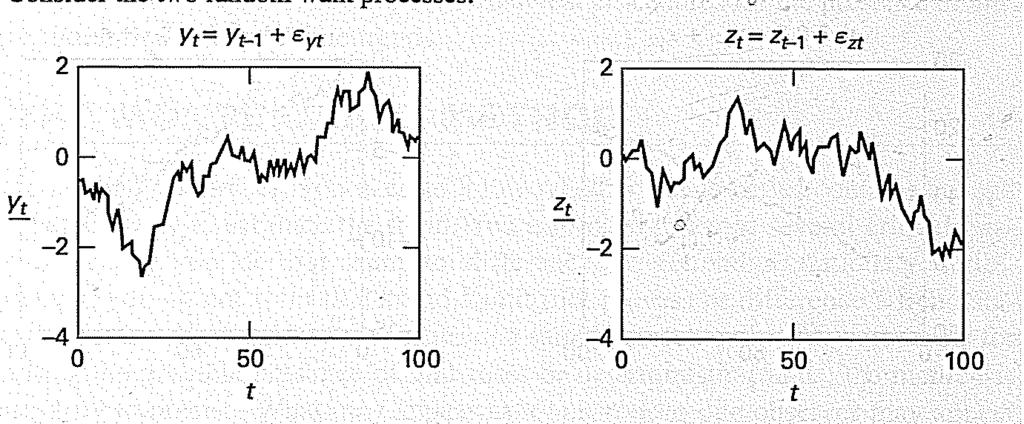
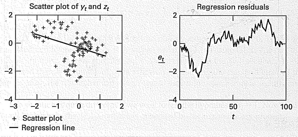
9 Spurious regression VIII

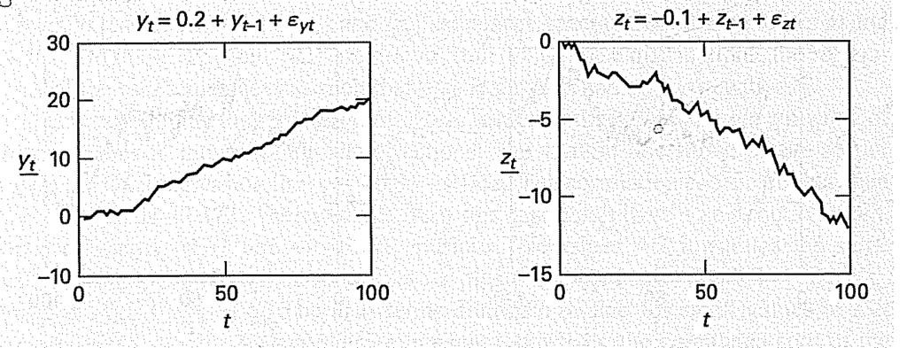
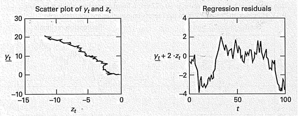
10 Spurious regression IX

11 Distinguishing Di erent Models I Consider the following data from four di erent models:

12 Distinguishing Di erent Models II It is clear that we cannot tell these apart by visual inspection. Will the ACF tell us that we are dealing with a unit root process? Consider the simple example: and y t = y t 1 + ε t, y t = y 0 + E (y t ) = y 0 t ε j j=1

13 Distinguishing Di erent Models III The autocovariance is: γ s = E [(y t y 0 ) (y t s y 0 )] " # t t s = E ε j ε i = (t s) σ 2 j=1 i=1 The variance is: V (y t ) = tσ 2 and therefore the ACF is r (t s) (t s) ρ s = p = (t s) t t

14 Distinguishing Di erent Models IV Note that as s increases the ACF falls, making it hard to tell the di erence between the unit root process and an AR process, even when the errors are white noise. For a trend model: and y t = α + δt + u t E (y t ) = α + δt V (y t ) = V (u t )

15 Distinguishing Di erent Models V So and γ s = E [(y t (α + δt)) (y t s (α + δ (t s)))] = E (u t u t s ) ρ s = E (u tu t s ) V (u t ) V (u s ) So the ACF re ects the ACF of the error process. Clearly recognizable if the error process is white noise... The rst investigation to distinguish between these two types of series was made using the ACF of the residuals series tted to either stochastic or deterministic trends.

16 Distinguishing Di erent Models VI Consider the following estimation on real GDP data: rgdp t = t t t 3 The graph of the data and the tted values looks like:

17 Distinguishing Di erent Models VII If we just eyeball, this seems like a very good model. An alternative estimation is: ln (rgdp t ) = ln (rgdp t 1 ) ln (rgdp t 2 ) The ACF and PACF from the residuals look like:

18 Distinguishing Di erent Models VIII

19 Distinguishing Di erent Models IX Clearly there is a lot of persistence left after de-trending, even though the t looked very good, where as the estimated unit root model seems to have residuals that behave like white noise. This point was rst made by Nelson and Plosser in They tted thirteen important macroeconomic series that had been treated as trend-stationary up until that point.

20 Unit Root Testing in a Simple Model I Consider the very simple model y t = α + ρy t 1 + ε t We know we cannot use standard hypothesis testing to test ρ = 1. (Although ρ = 0 would work). Especially with OLS we know that our estimates of ρ are downwards biased, making the model look more like a stationary AR (1) process. The asymptotic distribution of ˆρ can be found, but it has no nice closed form. It turns out that we can use the computer to nd the distribution under the null of ρ = 1. How?

21 Unit Root Testing in a Simple Model II You generate data according to y t = α + y t 1 + ε t Then you estimate y t = α + ρy t 1 + ε t using OLS and record the value of ˆρ and s 2, or, more importantly t = ˆρ 1 q s 2 (y t 1 ȳ) 2 You repeat this process many times and keep the results.

22 Unit Root Testing in a Simple Model III Dickey and Fuller found that 90% of the time t was less than % of the time t was less than % of the time t was less than 3.51 How do you use this information to carry out tests? What type of mistake would we have been making if we used standard normal critical values? How would you create a two-sided test? Caution: These methods only work if a CLT actually applies! It is also nessesary to investigate how the assumptions under which you generated the data a ects the reults. In this case: Do the numbers depend on the exact distribution of ε t? Do the numbers depend on the value of α used to generate the data?

23 Dickey-Fuller Tests I A little about Dickey and Fuller and Iowa State. Dickey and Fuller considered three di erent models: y t = γy t 1 + ε t (1) y t = a 0 + γy t 1 + ε t (2) y t = a 0 + γy t 1 + a 2 t + ε t (3) Note that (1) is equivalent to the model we considered last section. The hypothesis of interest now is H 0 : γ = 0. The alternative we are considering is H A : γ < 0. Typically we ignore the possibility that y t = y t 1 + ε t, even though, stricly speaking, this is also a unit root.

24 Dickey-Fuller Tests II To test γ = 0, we simply calculate the standard t statistic. Unfortunately the critical values are di erent for the three di erent models above. The t-test statitistic for the three models above are ususally labelled: τ, τ µ and τ τ. Dickey and Fuller also provide critical values for F test of joint hypotheses in these three models. We will apply these in an example later.

25 Augmented Dickey-Fuller Tests I Clearly AR (1) models are not always su cient to describe our data. Consider an AR (p) process: y t = a 0 + a 1 y t 1 + a 2 y t a p y t p + ε t We can rewrite this model in the following way: y t = a 0 + a 1 y t a p 1 y t p+1 + a p y t p+1 a p y t p+1 + ε t = a 0 + a 1 y t (a p 1 + a p ) y t p+1 a p y t p+1 + ε t = a 0 + a 1 y t a p 2 y t p+2 + (a p 1 + a p ) y t p+2 (a p 1 + a p ) y t p+2 a p y t p+1 + ε t

26 Augmented Dickey-Fuller Tests II y t = a 0 + a 1 y t (a p 2 + a p 1 + a p ) y t p+2 (a p 1 + a p ) y t p+2 a p y t p+1 + ε t = a 0 + (a a p 1 + a p ) y t 1 From this expression we get: (a a p 1 + a p ) y t 1... a p y t p+1 + ε t y t = a 0 + (a a p 1 + a p 1) y t 1 (a a p 1 + a p ) y t 1... a p y t p+1 + ε t = a 0 + γy t 1 + p i=2 β i y t i+1 + ε t

27 Augmented Dickey-Fuller Tests III where γ = β i = p i=1 p a j j=i a i! 1 and Again, we have a unit root if γ = 0. If this model is correctly speci ed we can use the critical values which applied to the simpler models.

28 Augmented Dickey-Fuller Tests IV This still leaves many important issues to deal with in the data: The model may contain unknown MA components. We need to have the right number of autoregressive lags. The data might be I (2) or higher. There might be structural breaks in the data. These can confuse and make it seem like otherwise stationary data has a unit root. We may not know whether to include the constant and trend in the model. Unknown MA components are reaonable simple to deal with. We can write an invertible ARMA process as an AR ( ) process, such that: y t = a 0 + γy t 1 + i=2 β i y t i+1 + ε t This we cannot estimate with nite samples...

29 Augmented Dickey-Fuller Tests V Dickey and Fuller have shown that an unknown ARIMA (p, 1, q) process can be well approximated by an ARIMA (n, 1, 0), where n T 3 1. Clearly we can estimate an ARIMA T 1 3, 1, 0 with a dataset of T observations.

30 Augmented Dickey-Fuller Tests I Lag-length Selection An important practical issue for the implementation ofthe ADF test is the speci cation of the lag length p. If p is too small then the remaining serial correlation in the errors will bias the test. If p is too large then the power of the test will su er. (Why?) Monte Carlo experiments suggest it is better to err on the side of including too many lags. A standard method for lag selection is: Set an upper bound p max for p. Estimate the ADF test regression with p = p max.

31 Augmented Dickey-Fuller Tests II Lag-length Selection If the absolute value of the t statistic for testing the signi cance of the last lagged di erence is greater than 1.6 then set p = p max and perform the unit root test. Otherwise, reduce the lag length by one and repeat the process. A common rule of thumb for determining p max, suggested by Schwert (1989), is p max = " 12 1 # T where [x] denotes the integer part of x. Note that this choice is completely ad hoc! Remember to check that the residuals look like white noise after selecting a lag length (regardless of selection method...)

32 Augmented Dickey-Fuller Tests III Lag-length Selection A di erent way to determine lag length is to use information criteria. The standard AIC and SBC are often used. Example of lag length selection. 200 observations were generated by: y t = y t y t 3 + ε t Here the series does contain a unit root and the correct lag length is 3. The data looks like:

33 Augmented Dickey-Fuller Tests IV Lag-length Selection

34 Augmented Dickey-Fuller Tests V Lag-length Selection Seeing this data we clearly cannot tell whether or not to include a trend, so we estimate: y t = a 0 + a 2 t + γy t 1 + p i=2 β i y t i+1 + ε t The estimation results are:

35 Augmented Dickey-Fuller Tests VI Lag-length Selection For this model the critical value for the DF test is t test < 3.43) SBC and AIC do not agree on the lag length choice (Reject if It turns out, however, that this does not a ect the conclusion of the unit root test... The φ 2 statistic tests the hypothesis that a 0 = a 2 = γ = 0 and the φ 3 statistic tests the hypothesis that a 2 = γ = 0. The critical values are 4.88 and As a result we do reject the presence of a trend, but not the presence of a constant. If we had tested this model with t and F tests, β 4 = 0, β 3 = β 4 = 0 and so forth, we would have concluded that we should have included 2 lags.

36 Augmented Dickey-Fuller Tests VII Lag-length Selection Also note that had we used four lags, we would not have been able to reject a 0 = a 2 = γ = 0. This is because of the reduced power of the test. Finally note that he current state of the art for lag selection was introduced by Ng and Perron in This critereon is the MAIC (k).