EASTERN MEDITERRANEAN UNIVERSITY ECON 604, FALL 2007 DEPARTMENT OF ECONOMICS MEHMET BALCILAR ARIMA MODELS: IDENTIFICATION

Transcription

1 ARIMA MODELS: IDENTIFICATION A. Autocorrelations and Partial Autocorrelations 1. Summary of What We Know So Far: a) Series y t is to be modeled by Box-Jenkins methods. The first step was to convert y t to stationary series x t and zero-mean series z t. 1) Consecutive and seasonal differencing or other deterministic transformations of y t yielded stationary series x t, where E(x t ) = μ and Var(x t ) = σ 2. 2) For ARMA modeling, we write x t = μ + z t, where z ~ ARMA(p,q). 3) We estimate μ with x, then compute series z t = x t x. 4) z is stationary, with E(z t ) = and Var(z t ) = Var(x t ) = σ 2. b) The next step is to identify the ARMA process that might have generated z t. 1) z ~ ARMA(p,q): z t = φ 1 z t φ p z t-p + ε t + θ 1 ε t θ q ε t-q, ε ~ WN(, σ 2 ε). 2) The principal tool of identification is the pattern in the autocorrelations (ρ h ) and partial autocorrelations (φhh) of z. Different processes have distinct patterns. 3) We use estimates and of z t, then look for a match with patterns of a known ARMA time-series generating process. c) Before proceeding with identification, we must know 2 things: What are autocorrelations and partial autocorrelations of a time series? What patterns in autocorrelation functions and partial autocorrelation functions (ACF and PACF) are associated with different ARMA models? 2. Autocorrelations and the ACF: a) We examined autocorrelations in Topic 5 when we defined stationarity as implying constant mean, variance and autocorrelations. 1) Given two random variables X and Y, covariance σ xy = E[(x-μ x )(y-μ y )] and correlation ρ xy = σ xy /σ x σ y. 2) In any time series y t, autocorrelation ρ t,t-h is the correlation between y t and previous value y t-h : ρ t,t-h = E[(y t -μ t )(y t-h -μ t-h )]/σ t σ t-h. 3) If z is stationary with zero mean, and constant variance σ 2 : ρ t,t-h = E(z t z t-h )/σ 2. 4) Furthermore, stationarity implies that ρ t,t-h = ρ h, constant over time; it depends only on the temporal displacement s and not on t: ρ 1 = Corr(z t,z t-1 ), ρ 2 = Corr(z t,z t-2 ); ρ h = Corr(z t,z t-h ) b) Estimating autocorrelations. 1) Start with y t, t = 1...T. Some observations are lost in differencing to arrive at stationary series x t and z t = x t x, t = τ...t. Let n = number of remaining observations. For successful ARIMA forecasting, we need n 75 or so. 1

2 2) Estimate true autocorrelations ρ h with sample autocorrelations, where s h is the estimated or sample cov(z t,z t-h ) and s 2 is the sample variance of z: T zt zt h T t= h+ 1 s ˆ ρ = = T 2 zt s T h h 2 t= 1 for large T 3) Note that we could get essentially the same estimates by running the following series of OLS regressions: z t = α + βz t-1 + u t : = z t = α + βz t-2 + u t : = z t = α + βz t-h + u t : = 3. Partial Autocorrelations and the PACF: a) Partial autocorrelation in time-series analysis. 1) Ordinary autocorrelations ρ h = E(z t,z t-h )/σ 2 measure the overall linear relationship between z t and z t-h. 2) The s-order partial autocorrelation φ hh measures that part of the correlation ρ h between z t-h and z t not already explained by ρ 1, ρ 2,..., ρ h-1. b) Let s illustrate with z t = φ 1 z t-1 + φ 2 z t-2 + ε t. Recall that ε ~ WN(,σ 2 ε), so ε t is not correlated with past values ε t-h or z t-h. 1) z t is related to z t-2 in two ways. Direct dependence through φ 2 z t-2 Indirect dependence through φ 1 z t-1 because z t-1 = φ 1 z t-2 + φ 2 z t-3 + ε t-1. 2) Now note that: ρ 2 = E(z t z t-2 )/σ 2 = E[(φ 1 z t-1 + φ 2 z t-2 + ε t )z t-2 ]/σ 2 = E(φ 1 z t-1 z t-2 + φ 2 z t ε t z t-2 )/σ 2 = φ 1 ρ 1 + φ 2 3) Thus, part of ρ 2 is determined by ρ 1. φ 22 is that part of ρ 2 not explained by ρ 1. 4) Similarly, φ 33 is that part of ρ 3 which is not already determined by ρ 1 and ρ 2, etc. 5) Incidentally, φ 11 ρ 1. [Why?] c) Estimate partial autocorrelations with series of OLS regressions: z t = α + β 1 z t-1 + u t : z t = α + β 1 z t-1 + β 2 z t-2 + u t : : z t = α + β 1 z t-1 + β 2 z t βhz t-h + u t : 4. Standard Errors of Estimators and and Hypothesis Tests: a) If true = =, then for large T, sampling distributions of and are normal with mean and standard error se( ) = se( ) = 1/ T: and ~ N(,1/T) 2

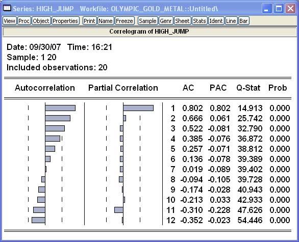
3 b) Consider hypothesis tests H : (or ) = ; H 1 : (or ). If -2/ T < or < 2/ T, do not reject H at 5% level of significance c) Ljung-Box Test (Portmanteau Test) A test that first h autocorrelations are jointly zero : against : for at least one 1,, Test statistics: 2 ~ Example: Olympic, high jump data Date: 9/3/7 Time: 16:15 Sample: 1 2 Included observations: 2 Autocorrelation Partial Correlation h AC PAC Q-Stat Prob. ******. ****** ***** ****. * ***. * **.. * *.. * * *.. * * ** **..** ***

4 4

5 B. ACF and PACF Patterns in Nonseasonal ARMA Processes 1. Introduction: a) A stationary series x t has been obtained, t = 1...T. b) The correlogram of x is a table and graph representing its estimated autocorrelation function (ACF) and partial autocorrelation function (PACF), showing and along with the ± 2 SE bounds (where SE = 1/ T). Correlogram of X Included observations: T = 59 Autocorrelation Partial Correlation s AC PAC Q-Stat Prob ****. **** ** * * **..* ** * *..* c) Now we try to match patterns in the correlogram with patterns of known ARMA processes to identify the ARMA(p,q) model which might have generated x. The patterns to look for are presented in the next sections below. Recall that: Correlograms of x t and z t = x t x are identical Var(x) = var(z) = σ 2 ε ~ WN(, σ 2 ε) d) Remember that when working with actual data series, correlograms are based on estimates and. Patterns in the estimated ACF and PACF will rarely be crystal clear. 2. First-Order Autoregressive Processes: a) z ~ ARMA(1,) or just AR(1): z t = φz t-1 + ε t or (1-φL)z t = ε t b) Mean and variance. 1) E(z t ) = 2) Var(z t ) = σ 2 = σ 2 ε/(1-φ 2 ). Proof: Var(z t ) = E(z t 2 ) = E[(φz t-1 + ε t ) 2 ] = E[φ 2 z t φε t z t-1 + ε t 2 ] = φ 2 σ σ 2 ε c) Theoretical ACF. 1) ρ 1 = Corr(z t,z t-1 ) = E(z t z t-1 )/σ 2 2) E(z t z t-1 ) = E[(φz t-1 + ε t )z t-1 ] = E(φz t ε t z t-1 ) = φσ 2 + 3) Hence, ρ 1 = φ. 4) It is easy to show that ρ 2 = E(z t z t-2 ) = φ 2, and that, in general, ρ h = σ h. 5

6 5) Since stationarity implies that φ < 1, the ρ h decay to (die out geometrically), possibly with oscillations, from lag h = 1. d) Theoretical PACF. 1) As with all processes, φ 11 ρ 1, which in this case = φ. 2) z t is correlated with z t-2 because z t is a function of z t-1, and z t-1 = φz t-2 + u t-1. But is there any correlation between z t and z t-2 that is not through the influence of z t-1, which is what φ hh would measure? The answer is no, because ρ 2 = φ 2 = φρ 1 and, in general, ρ h = φ h = φρ h-1. There is no part of the dependence of z t on z t-h that is not explained ρ 1, ρ 2,..., ρ h-1. 3) Hence, φ hh =, h > 1. The φ hh cut off after lag h = 1. Theoretical ACF -- AR(1) Theoretical PACF -- AR(1) Autocorrelation Rs Partial Autocorrelation Rss Processes: Lag h s -.4 Lag sh 2. Second and Higher-Order Autoregressive a) z ~ ARMA(p,) or just AR(p): z t = φ 1 z t φ p z t-p + ε t b) Theoretical ACF and PACF patterns for AR(p) processes. 1) ρ h eventually decay to (die out geometrically) possibly with oscillations and perhaps not uniformly. 2) As with all processes, φ hh ρ 1. Also, φ pp = φ p. 3) All φ hh = (cut off) for lags h > p. Theoretical ACF -- AR(2) Theoretical PACF -- AR(2) Autocorrelation Rs Partial Autocorrelation Rss Lag h s Lag sh

7 3. First-Order Moving Average Process: a) z ~ ARMA(,1) or just MA(1): z t = ε t + θε t-1 or z t = (1+θL)ε t b) Mean and variance. 1) E(z t ) = 2) Var(z t ) = σ 2 = (1+θ 2 )σ 2 ε. Proof: Var(z t ) = E(z t 2 ) = E[(ε t + θε t-1 ) 2 ] = E(ε t 2 + 2θε t ε t-1 + θ 2 ε t-1 2 ) = σ 2 ε + + θ 2 σ 2 ε c) Theoretical ACF. 1) ρ 1 = Corr(z t,z t-1 ) = E(z t z t-1 )/σ 2 2) E(z t z t-1 ) = E[(ε t + θε t-1 )( ε t-1 + θε t-2 )] = E(ε t ε t-1 + θε t ε t-2 + θε t θ 2 ε t ε t-2 ) = + + θσ 2 ε + = θσ 2 ε 3) Hence, ρ 1 = θσ 2 ε/σ 2 = θσ 2 ε/[(1+θ 2 )σ 2 ε] = θ/(1+θ 2 ) ½. 4) It is easy to show that ρ 2 = E(z t z t-2 ) = and that, in general, ρ h =, h > 1. The ρ h cut off after lag h = 1. d) Theoretical PACF. 1) As with all processes, φ 11 ρ 1, which in this case = θ/(1+θ 2 ) 1/2. 2) The φ hh die out geometrically, possibly with oscillations, from lag h = 1. [See explanation below.] Theoretical ACF -- MA(1) Theoretical PACF -- MA(1).1.1 Autocorrelation Rs Partial Autocorre lation Rss Lag h s -.6 Lag h s e) To understand why the PACF dies out, we must consider something new, called the invertibility condition for an MA(q) process. 1) An MA(1) process can be inverted to an AR( ) process by back substitution: z t = ε t + θε t-1 => ε t = z t θε t-1 = z t θ(z t-1 θε t-2 ) =... Rearranging, we eventually get z t = ε t + θz t-1 + θ 2 z t-2 + θ 3 z t

8 2) The z ~ AR( ) process is convergent only if θ < 1, the so-called invertibility condition for MA(1) processes. We will avoid further discussion of invertibility as things are already complicated enough. But from the AR( ) process, we see that z is correlated with all its past values z t-h, and that they are dying out because θ h as h. But none of this correlation is determined by direct autocorrela-tions ρ 2, ρ 3,... ρ h-1, which all =. All of it is partial autocorrelation φ hh. 4. Second and Higher-Order Moving Average Processes: a) z ~ ARMA(,q) or just MA(q): z t = ε t + θ 1 ε t θ q ε t-q b) Theoretical ACF and PACF patterns for MA(q) processes. 1) ρ h = (cut off) for lags h > q. 2) As with all processes, φ 11 ρ 1. 3) φ hh eventually decay to (die out geometrically), possibly with oscillation and perhaps not uniformly. 4) For a sample diagram, switch the ACF/PACF patterns of the AR(2) model above. 5. Mixed ARMA(1,1) Process: a) z ~ ARMA(1,1): or (1-φL)z t = (1+θL)ε t b) Mean and Variance. 1) E(z t ) = 2) Var(z t ) = σ 2 = [(1+θ 2 +2φθ)/(1-φ 2 )]σ 2 ε. Proof: [Left as exercise] Var(z t ) = E(z t 2 ) = E[(ε t + θε t-1 ) 2 ] = E(ε t 2 + 2θε t ε t-1 + θ 2 ε t-1 2 ) = σ 2 ε + + θ 2 σ 2 ε c) Theoretical ACF and PACF patterns for ARMA(1,1) processes. (1 + ϕθ)( φ + θ ) 1) ρ 1 = and ρh = ϕρ 1 2 Proof left as excercise 2 h h 1+ θ + 2ϕθ 2) Thus, ρ h decay to (die out geometrically), possibly with oscillation, starting from lag h = 1. 3) As with all processes, φ 11 ρ 1. 4) φ hh decay to (die out geometrically), possibly with oscillation, from lag h = 1. 8

9 Theoretical ACF -- ARMA(1,1) Theoretical PACF -- ARMA(1,1) Autocorrelation Rs Partial Autocorrelation Rss Lag Lag h s -1 Lag s 6. Mixed ARMA(p,q) Processes: a) z ~ ARMA(p,q): z t = φ 1 z t φ p z t-p + ε t + θ 1 ε t θ q ε t-q b) Theoretical ACF and PACF patterns for ARMA(p,q) processes. 1) ρ h eventually decay to (die out geometrically), possibly with oscillation, beginning from lag h = q. 2) As with all processes, φ 11 ρ 1. 3) φ hh eventually decay to (die out geometrically), possibly with oscillation, beginning from lag h = p. Theoretical ACF -- ARMA(2,3) Theoretical PACF -- ARMA(2,3) Autocorrelation Rs Partial Autocorrelation Rss Lag h s -.3 Lag Lag h h s 7. Seasonal ARIMA Processes: a) ARIMA models. 1) Suppose that original series y t is differenced d times to get stationary series x t and x ARMA(p,q). 9

10 2) Then we write y ARIMA(p,d,q). b) Seasonal ARIMA models. 1) If y t is nonstationary in part due to seasonality of length M, both D seasonal and d consecutive differences may be required to reach stationarity. For d = D = 1: x t = (1-L)(1-L s )y t = (y t - y t-1 ) - (y t-m - y t-m-1 ) = Δy t Δy t-s 2) Even after differencing, the generating process of x t may still include seasonal SAR(P) and SMA(Q) terms. If x t is generated by a mixture of ARMA(p,q) and SARMA(P,Q) processes, we write: x ARMA(p,q)(P,Q) and y ~ ARIMA(p,d,q)(P,D,Q) 3) Suppose z = x-μ ARMA(1,1)(1,1) and M = 4. Then the model has ARMA parameters φ and θ and seasonal SARMA parameters Φ and Θ: (1-φL)(1-ΦL 4 )z t = (1-θL)(1-ΘL 4 )ε t or (z t -φz t-1 ) - Φ(z t-4 -φz t-5 ) = (ε t -θε t-1 ) - Θ(ε t-4 -θε t-5 ) 1

11 Here are some more examples of ACF and PACF patterns: EXAMPLE ACF EXAMPLE PACF SUGGESTED MODEL FORM AR(1) (1 - Φ 1 L 1 ) (x t - μ) = ε t AR(2= (1- Φ 1 L 1 - Φ 2 L 2 ) (x t - μ) = ε t AR(4) (1- Φ 1 L 4 ) (x t - μ) = ε t MA(1) (x t - μ) = (1- θ 1 L 1 ) ε t MA(4) (x t - μ) = (1- θ 1 L 4 ) ε t AR1MA(1,4) (1- Φ 1 L 1 ) (x t - μ) = (1- θ 1 L 4 ) ε t As illustrated above, matching up patterns in observed sample ACF's and PACF's with theoretical models can sometimes be a bit of a challenge. An approach is to implement a search and- capture heuristic which evaluates alternatives and then selects the best model using decision rules based upon the AIC criteria and the error sum of squares. This rule-based system then can be used to automatically identify the initial model. 11

12 IDENTIFICATION OF ARMA MODELS: A SUMMARY OF PROPERTIES OF THE AC AND PAC FUNCTIONS (Adapted from Enders, page 85) PROCESS ACF PACF White noise All ρ h = All φ hh = AR(1): φ 1 > Direct exponential decay: φ 11 = φ 1; φ hh = for k 2 h ρ h = φ 1 AR(1): φ 1 < κ Oscillating decay: ρ k = φ 1 φ 11 = φ 1; φ hh = for k 2 AR(p) Decays towards zero. Coefficients may oscillate. Spikes through until lag p, followed by cut off in PAC function beyond lag p. φ hh for k p. φ hh = for k > p. MA(1): θ 1 < Negative spike at lag 1. Exponential decay: φ 11 < ρ h = for h 2 MA(1): θ 1 > Positive spike at lag 1. ρ h = for h 2 Exponential decay: φ 11 > MA(q) ARMA(1,1) : φ 1 > ARMA(1,1) : φ 1 < ARMA(p,q) ρ h for h q ρ h = for h > q i.e. a cut-off in the ACF Exponential decay beginning at lag 1 Oscillating decay beginning at lag 1 Decay (either direct or oscillatory) at lag q φ hh taper off Oscillatory decay beginning at lag 1. φ 11 = φ 1 Exponential decay beginning at lag 1. φ 11 = φ 1 Decay (either direct or oscillatory) beginning at lag p, but no distinct cut-off point. I(1) or I(2) series ρ h tapers off very slowly or not at all 12

13 In summary, the autocorrelation function (ACF) and partial autocorrelation function(pacf) shows the following behavior for causal and invertible ARMA models: AR(p) MA(q) ARMA(p,q) ACF Tails off Cuts off after lag q Tails off PACF Cuts off after lag p Tails off Tails off Therefore, * If the ACF cuts off after lag q, we have an MA(q) model. * If the PACF cuts off after lag p, we have an AR(p) model. * If neither the ACF nor the PACF cut off, then we have an ARMA model. Here the ACF and PACF provide little useful information for determining p and q. 13