Econometrics Lecture 9 Time Series Methods

Transcription

1 Econometrics Lecture 9 Time Series Methods Tak Wai Chau Shanghai University of Finance and Economics Spring / 82

2 Time Series Data I Time series data are data observed for the same unit repeatedly over time. I Example: macro variables such as GDP, in ation, unemployment, exports, or nancial data like stock price, bond price, exchange rate. I Denote time for each observation as t = 1, 2,..., T. I The most notable di erence for time series data is that, there is a natural ordering according to time. The order in cross-sectional data is arbitrary. I It may be helpful to plot the time series against time. I There can be dependence across observations over time. It is not as reasonable as in cross-sectional data to assume independence across observations. I Current value may depend on the past values of itself and other variables. We call them lagged variables. 2 / 82

3 3 / 82

4 Time Series Data I We call a time series strongly stationary if the joint distribution of a segment of time series z t, z t+1,..., z t+k does not depend on t for any k = 0, 1,... I We call a time series weakly stationary (or covariance stationary) if the unconditional mean E (z t ), variance Var(z t ), and all covariances cov(z t, z t k ) for all k = 1, 2,... do not depend on time t. I If the series is not stationary, it may have a trend. I Be cautious about relations between variables with trends. I Two variables having upward or downward trend may seem to have strong relation with each other in a regression (e.g very high R 2 and t statistics), but they may not be closely related when having a closer look. I If two variables have causal relations, we would expect they are still closely related even after taking away the trend. 4 / 82

5 Time Series Data I Here I mainly brie y discuss two aspects: I 1) Static model. Adjustments to the OLS assumptions under time series data, and the consequences if the error term are serially correlated. I 2) Models with lagged variables as regressors. We call these dynamic models. (e.g. ARDL.) I 3) Stochastic trends, unit root and cointegration. 5 / 82

6 Time Series Data I Some useful terminology and transformations: I We call y t j the j th lag of y t. Sometimes we write y t j = L j y t, where L is called the lag operator. I We call y t = y t y t 1 the rst di erence of y t. I When we consider the log transformation, the rst di erence in log is the approximated growth rate if it is not too large: ln y t = ln y t ln y t 1 = ln(y t /y t 1 ) yt y t 1 = ln + 1 y t 1 ' y t y t 1 y t 1 since ln(1 + x) ' x for small x. I First di erences, like growth rates, are less a ected by the trend over time. e.g. growing at a xed percentage becomes a constant now. 6 / 82

7 7 / 82

8 Autocorrelation I A useful concept about time series is autocorrelation. I For a time series y t, t = 1, 2,..., T, the j th autocovariance is cov(y t, y t j ), and so the j th autocorrelation is corr(y t, y t j ) = ρ j = cov(y t, y t j ) p Var(yt )Var(y t j ) = cov(y t, y t j ) Var(y t ) and the last equality holds for weakly stationary series. I The sample covariance can be obtained from a sample dcov(y t, y t j ) = 1 T T (y t ȳ j+1,t )(y t j ȳ 1,T j ) t=j+1 where ȳ s,t is the sample average from period s to period t. I The sample autocorrelation is given by ˆρ j = dcov(y t, y t j ) dvar(y t ) where Var(y t ) = cov(y t, y t 0 ). 8 / 82

9 Basic Assumptions I Consider the regression model y t = x 0 t β + ε t I Some assumptions can be maintained, but some may need modi cations. I These can be maintained: I Assumption 1: The regression function is linear in parameters I Assumption 3: There is no perfect multicollinearity among regressors. I Assumption 5: Errors ε t are homoscedastic. I But the other assumptions should be adjusted to allow for broader situations. 9 / 82

10 Basic Assumptions I Assumption 2 is originally about independence across each observation or unit. I But for time series, the same unit is sampled repeatedly over time, so they are generally not independent. I e.g. When the unemployment rate is higher than normal this quarter, it is likely that it will also be higher than normal the next quarter. I We may replace with this: I Assumption 2 (Stationary Time Series) {(y t, x t ) : t = 1,..., T } are stationary and weakly dependent. I Weakly dependent roughly means the dependence over time (e.g. autocorrelation) dies down to zero when the time in between increases to in nity. I This guarantees some forms of LLN and CLT to apply. Technical details are skipped. 10 / 82

11 Basic Assumptions I Assumption 4 is the zero conditional mean assumption. I Strict exogeneity: E (ε t jx 1,..., x T ) = 0, that means values of regressors for all observations do not give us more information about the error of a period. I This is required for the unbiasedness of the OLS estimator. I But it may be too strict in some cases. e.g. It is violated when one of the regressors in x t is a lagged dependent variable y t 1. I So, usually weak exogeneity is assumed: E (ε t jx t ) = 0. I This is enough for consistency. I For dynamic models, it is also reasonable to have E (ε t jx t 1,..., x 1 ) = 0, where x t are known as pre-determined variables. (x t refers to regressors in general, which can include y t j.) I This means the values of regressors in the past do not a ect the errors now and for the future. We call such ε t a shock. 11 / 82

12 Basic Assumptions I Before in the basic assumptions, independent observation implies no correlation among the error terms. I For time series, we need an extra assumption to include this: I Assumption 6: No serial correlation cov(ε t, ε s ) = 0 for all s, t = 1,..., T. I But we can also allow this to be violated. I If we just want a static model where no lag variables are included, then we can allow the error to be serially correlated because of the correlation of the unobserved variables over time. I For a dynamic model, when lag dependent variables are included to capture the dynamics, then we will use enough lagged variables so that the error terms are uncorrelated. 12 / 82

13 Properties of OLS I For unbiasedness, we need strict exogeneity E (ε t jx 1,..., x T ) = 0. If it fails, the OLS estimator is not unbiased. I But if we have reasonably large sample, consistency just requires weak exogeneity E (ε t jx t ) = 0. I So, in the case of lagged dependent variable as a regressor, we can only have consistency. I Note that, if we have both serial correlation of error ε t and lagged dependent variable y t 1, weak exogeneity is not satis ed, and so there is inconsistency. I But if there is no lagged dependent variables, serial correlation in the error term does not a ect consistency. I For e ciency, Gauss-Markov Theorem only applies to the case with error homoscedastic and no serial correlation. I We will look at how to improve e ciency by GLS in case of serial correlation in errors. 13 / 82

14 Properties of OLS I For asymptotic properties, we need a version of Law of Large Numbers and Central Limit Theorem to hold when observations are dependent / correlated where the variables are only weakly dependent. I Technical details are not covered here. I The key is that if the dependence over time die down fast enough so that latter draws can carry enough new information to the sample mean, then a version of LLN and CLT holds. I If this is satis ed, the OLS estimator is consistent and asymptotically normal as before. I For models with trends, the LLN and CLT involved are di erent and much more complicated. They will be skipped in this class. 14 / 82

15 Serial Correlations I Now consider a static regression model with stationary variables, where only variables of the same t are included: y t = x 0 t β + ε t I If cov(ε t, ε t k ) 6= 0 for some k > 0, then we say the errors are serially dependent, or there is serial correlation in the error. I The dependence may come from the dependence of unobservable factors over time. I Sometimes we focus on long run relations and the deviation from this long run relation is in the error term. The adjustment towards this long run relation may take time and so the deviation can be serially correlated. I The OLS estimator is still consistent if cov(x t, ε t ) = 0. I But as the derivation of usual OLS variance formula requires uncorrelated errors, the variance formula should be adjusted under serial correlation. 15 / 82

16 Autocorrelation Robust Variance I To obtain a valid variance formula, we deal with the variance of the last term.! T 1 Var T x t ε t t=1 which equals E 1 T! T x t ε t t=1 1 T! 0! T x t ε t = E t=1 1 T 2 T s=1 T t=1 I We may want to use the former one, but when directly replacing ε by e, the OLS rst order condition implies 1 T! T x t e t = 0 t=1 which makes the outer product identically zero. ε t ε s x t x 0 s! 16 / 82

17 Autocorrelation Robust Variance I So, at least we have to impose some restrictions on the autocorrelations to obtain a valid variance estimator. I The usual one is the Newey-West heteroscedasticity and autocorrelation consistent estimator (HAC), where we assume that the serial correlation only substantially a ect the variance estimate when the two observations are separated by fewer than L periods. I The middle term is ˆV = 1 T T 2 et 2 x t xt 0 t=1 + 1 T 2 L l=1 T t=l+1 w l e t e t l (x t x 0 t l + x t l x 0 t) where w l = 1 l/(l + 1), thus a lower weight for longer lags. (To ensure the estimate matrix is positive de nite.) I A suggestion is L ' T 1/4. 17 / 82

18 Model for Serial Correlation I Autoregressive Process of Order 1 (AR(1)): ε t = ρε t 1 + u t where u t is stationary, zero mean and serially uncorrelated over time. We call such series white noise. I u t is also uncorrelated to ε t s for s > 0. So it is an unpredictable shock. I By successive substitution, we have I Thus ε t = ρ s ε t s + ρ s 1 u t s+1 + ρ s 2 u t s ρu t 1 + u t cov(ε t, ε t s ) = ρ s cov(ε t s, ε t s ) = ρ s var(ε t ) or autocorrelation of lack s = ρ s. I It goes to zero when s goes to in nity, as long as jρj < 1. I The closer the ρ to 1, the more persistence is the series. 18 / 82

19 Model for Serial Correlation I We may also consider AR(p) process: ε t = ρ 1 ε t 1 + ρ 2 ε t ρ p ε t p + u t Thus the current error term depends directly on the error terms p periods before plus a new shock. I Another model for stationary time series is a moving average model (MA). MA(1): ε t = u t + λu t 1 where the shock at one previous period can directly a ect the current ε t. cov(ε t, ε t 1 ) = cov(u t + λu t 1, u t 1, λu t 2 ) = λvar(u t 1 ) cov(ε t, ε t s ) = cov(u t + λu t 1, u t s, λu t s 1 ) = 0 for s > 1 I So, the covariance drops to zero for 2 or more lags. I Similarly we can have MA(q) models that allow q shocks in the past. 19 / 82

20 Tests for Autocorrelation I Suppose we suspect that the error term ε follows AR(p). I Lagrange Multiplier Test, also known as Breusch-Godfrey test: This test is based on regression of the (OLS) residuals. I First, obtain the residual series of the corresponding model e t = y t xtb. 0 I Second, do the following regression (for t p + 1) e t = x 0 t γ + α 1 e t 1 + α 2 e t α p e t p + v t I LM = (T p)r 2 which follows χ 2 distribution with degrees of freedom p asymptotically under the null of NO correlation to the past p lags. I One may also use an F or Wald test for α 1 =... = α p = 0. I If there is correlation between errors, it will show up as non-zero α 1,..., α p, and thus some explanatory power to e t. I Very often, we take p = / 82

21 Tests for Autocorrelation I A more traditional test if the Durbin-Watson Test, which mainly test for rst order autocorrelation. I The test statistic is d = T t=2(e t e t 1 ) 2 T t=1 e 2 t ' T 1 t=1 e2 t + T t=2 e 2 t 2 T t=2 e t e t 1 T t=1 e 2 t ' 2 T t=2 e 2 t 2 T t=2 e t e t 1 T t=1 e 2 t = 2(1 r) where r is sample correlation coe cient between e t and e t 1. I The di erences between T 1 t=1 e2 t, T t=2 e 2 t and T t=1 e 2 t are negligible if T is large. I So, if there is strong positive correlation, r tends to 1, and d tends to 0. I If there is strong negative correlation, d tends to 4. I If there is no correlation, then it is close to / 82

22 Tests for Autocorrelation I There is a table to check for critical values (d L, d U ), which depends on sample size (T ) and number of regressors (K) in the original model. I For positive correlation, d < d L we reject the null of no serial correlation. I d > d U we fail to reject the null. I In the middle then it s inconclusive. I For negative correlation, the critical values become (4 d L, 4 d H ). (Reject if d > 4 d L ) I Some software report the Durbin-Watson statistic routinely, but now more people use LM test for a formal test. I But it can still give you a guide how serious the autocorrelation is. I DW test should not be used if the regressors are not strictly exogeneous (e.g. with y t 1 as regressor.) 22 / 82

23 Example Consider the annual change in log of gasoline consumption per capita in the US between Regressors include change in log gasoline price, change in log disposable income per capita, change in log price of new cars, change in log price of old cars, change in log price of public transport and change in log price of consumer services. I use change because the original variables include upward trends.. reg dlng_pop dlnpg dlny_pop dlnpnc dlnpuc dlppt dlps Source SS df MS Number of obs = 51 F( 6, 44) = 9.43 Model Prob > F = Residual R squared = Adj R squared = Total Root MSE = dlng_pop Coef. Std. Err. t P> t [95% Conf. Interval] dlnpg dlny_pop dlnpnc dlnpuc dlppt dlps _cons / 82

24 Example Test of serial correlation: you may use the command directly:. predict eb, res (1 missing value generated). estat dwatson Durbin Watson d statistic( 7, 51) = estat bgodfrey Breusch Godfrey LM test for autocorrelation lags(p) chi2 df Prob > chi estat bgodfrey, nom Breusch Godfrey LM test for autocorrelation lags(p) chi2 df Prob > chi estat bgodfrey, nom lag(3) H0: no serial correlation H0: no serial correlation Breusch Godfrey LM test for autocorrelation lags(p) chi2 df Prob > chi H0: no serial correlation 24 / 82

25 Example Verify by auxiliary regression. reg eb l(1/3).eb dlnpg dlny_pop dlnpnc dlnpuc dlppt dlps Source SS df MS Number of obs = 48 F( 9, 38) = 1.16 Model Prob > F = Residual R squared = Adj R squared = Total Root MSE = eb Coef. Std. Err. t P> t [95% Conf. Interval] eb L L L dlnpg dlny_pop dlnpnc dlnpuc dlppt dlps _cons scalar NR2=e(N)*e(r2). dis NR dis chi2tail(3,nr2) / 82

26 Example Newey-West Standard Errors. newey dlng_pop dlnpg dlny_pop dlnpnc dlnpuc dlppt dlps, lag(3) Regression with Newey West standard errors Number of obs = 51 maximum lag: 3 F( 6, 44) = Prob > F = Newey West dlng_pop Coef. Std. Err. t P> t [95% Conf. Interval] dlnpg dlny_pop dlnpnc dlnpuc dlppt dlps _cons / 82

27 Feasible GLS Estimation I If you discover serial correlation, one may keep the OLS and use the Newey-West (HAC) standard errors. I If you do not want to use a dynamic model, you may also do feasible GLS to improve e ciency. I This is to transform the model so that the error terms of di erent time periods are no longer correlated. I Consider the case where error is AR(1): ε t = ρε t 1 + u t I Substitute back the regression equation, (y t x 0 t β) = ρ(y t 1 x 0 t 1β) + u t y t ρy t 1 = (x t ρx t 1 ) 0 β + u t I If we have an estimate ˆρ, we can run the above regression with t = 2, 3,..., T. It is known as the Cochrane and Orcutt procedure (C-O). I An estimate of ˆρ is obtained by regressing e t on e t 1 by OLS. 27 / 82

28 Feasible GLS Estimation I A slightly di erent procedure called Prais and Winsten procedure, which also make use of the rst observation. I Note that if the process is stationary, σ 2 ε = ρ 2 σ 2 ε + σ 2 u (1 ρ 2 )σ 2 ε = σ 2 u I First, the rst observation s error ε 1 is not correlated to u 2,..., u T. I Second, we want the regression to be homoscedastic. I So, we transform the rst observation as q q 1 ρ 2 y 1 = ( 1 ρ 2 x 1 ) 0 β + so that Var( p 1 ρ 2 ε 1 ) = (1 ρ 2 )σ 2 ε = σ 2 u. q 1 ρ 2 ε 1 I Observation 2 to T are the same as C-O procedure above. 28 / 82

29 Example FGLS: Prais and Winsten. prais dlng_pop dlnpg dlny_pop dlnpnc dlnpuc dlppt dlps Iteration 0: rho = Iteration 1: rho = Iteration 2: rho = Iteration 3: rho = Iteration 4: rho = Iteration 5: rho = Iteration 6: rho = Iteration 7: rho = Iteration 8: rho = Iteration 9: rho = Iteration 10: rho = Iteration 11: rho = Prais Winsten AR(1) regression iterated estimates Source SS df MS Number of obs = 51 F( 6, 44) = Model Prob > F = Residual R squared = Adj R squared = Total Root MSE = dlng_pop Coef. Std. Err. t P> t [95% Conf. Interval] dlnpg dlny_pop dlnpnc dlnpuc dlppt dlps _cons rho Durbin Watson statistic (original) Durbin Watson statistic (transformed) use the option corc if you just want the C-O procedure. 29 / 82

30 Models with Lagged Variables I We can also allow multivariate models where we have another variables as regressors. I Here, we consider to put in the past values of regressors or dependent variable or both into the regression. I We call such model a dynamic regression model. I Reasons to put in lag values: 1. The e ect is dynamical in nature. Adjustments may take time, so the e ect may change some time after the cause changes. Its e ect takes time to fully realize. 2. There may be state dependent, or inertia that, for example, once a variable gets to a low value, it takes time to rise back. 3. Response may be a ected by expectations, which is formed by the past values of variables. (e.g. expectation augmented Philips curve) 30 / 82

31 Models with Lagged Variables I Here we consider stationary series. I If we put lags of independent variable, we call the model distributed lag model. I Consider a model also with x one period before: y t = α + β 0 x t + β 1 x t 1 + ε t I Then the contemporaneous (same period, immediate) e ect of x t on y t is β 0. I If x t 1 is one unit higher, holding x t unchanged, the e ect on y t is β 1. I So, if there s a temporary (single period) 1-unit increase in x t, y t increases by β 0 and y t+1 increases by β 1, and change nothing else. Thus, the total e ect is β 0 + β 1. I A permanent (all-period) increase in x t would change y t by β 0 + β 1 for every period, after 2 periods of adjustment. 31 / 82

32 Models with Lagged Variables I More generally, for a distributed lag model with p lags y t = α + β 0 x t + β 1 x t 1 + β 2 x t β p x t p + ε t I The contemporaneous e ect (for a unit change in x t ) is β 0. I The e ect to the next period is β 1. The e ect at s periods (s p) after is β s. I For a temporary (single period) change in x, the total e ect to the variable y over time is p s=0 β s. I For a permanent change in x, the e ect to y every period is also p s=0 β s after p periods of adjustment since all x and its lags on the RHS increases by 1. I We can also think in terms of a steady state (y 0, x 0 ) where x and y no longer change, which may be taken as a long-run equilibrium after adjustment completed. y 0 = α + β 0 x β p x 0 = α + ( p s=0 β s )x 0 32 / 82

33 Models with Lagged Variables Here all β 0 s are negative. 33 / 82

34 Models with Lagged Variables I If instead, we include a lagged dependent variable, we call it an autoregressive model: y t = α + βx t + γy t 1 + ε t where as before stationarity requires jγj < 1 I The one-unit increase in x t leads to a contemporaneous change in y t by β. I However, when it changes y t, which is also in the y t+1 equation, there is an e ect to y t+1 of γβ. I Similarly, when it changes y t+1,which enters the y t+2 equation, there is an e ect to y t+2 is γ 2 β, and so on. I So, the total e ect to y for a temporary change in x is β + γβ + γ 2 β +... = s=0 βγ s = β/(1 γ) I Similarly, it is also the long run e ect for a one-unit permanent change in x. 34 / 82

35 Models with Lagged Variables I Viewing the long run e ect in another way, after all the adjustments, and neglect temporary shocks ε t, it attains a steady state y t 1 = y t = y 0. I Also assume x is xed over time. I Then, y 0 = α + βx + γy 0 (1 γ)y 0 = α + βx y 0 = α 1 γ + β 1 γ x I Thus a permanent change in x by one unit leads to a change of y in the long run by β/(1 γ). I Also note that the constant term α here actually means the steady state constant term is α/(1 γ). 35 / 82

36 Models with Lagged Variables I So, there are a few reasons we put lagged of the dependent variable into the model: 1. An approximation to the e ect of x that dies down slowly in a similar pattern. 2. There is state dependent. When the value is lower (experiencing a negative shock), it takes some time to rise back. Similarly for a positive shock. 3. Partial adjustment to the optimal level. Assume the optimal level as y t = α + βx t + ε t and the adjustment takes y t y t 1 = γ(y t y t 1 ) Then the resulting equation becomes y t = αγ + (1 γ)y t 1 + γβx t + γε t 36 / 82

37 Models with Lagged Variables I If y t 1 is a regressor, the past error ε t 1 would be correlated to the present regressor y t 1. Thus strict exogeneity cannot be satis ed, and OLS estimator fails to be unbiased. I But as stated before, weak exogeneity, which means regressors of the current equation are not correlated to the current error, is enough for consistency. I Here, we need E (ε t jy t 1, x t ) = 0. I Usually true if it can be understood as a shock: something that cannot be predicted beforehead. I Moreover, if ε t are serially correlated, say cov(ε t, ε t 1 ) 6= 0, then models with lagged dependent variable would fail even to be consistent. cov(y t 1, ε t ) = cov(α + βx t 1 + γy t 2 + ε t 1, ε t ) = cov(ε t 1, ε t ) 6= 0 I In this case, one should use IV, or respecify the model with more lags of either x or y to capture this dependence. 37 / 82

38 Models with Lagged Variables I In general, we can have autoregressive distributive lag model (ARDL): y t = α + p s=1 γ s y t s + q j=0 β j x t j + ε t I This would give us various forms of dynamic e ects for a change in x,α or ε. I As before, these models can be estimated by OLS, if weak exogeneity is satis ed. I The long run e ect of a permenant change in x can be expressed as so y 0 = α + p s=1 y 0 α = 1 p s=1 γ s γ s y 0 + q j=0 β j x 0 + q j=0 β j 1 p s=1 γ x 0 s 38 / 82

39 Selecting Speci cations A few concerns for selecting appropriate speci cations, especially about how many lags to use: I Theorectical concern: Is there any suggestions from theory? I The error term is a white noise (serially uncorrelated), so that any useful information from the past has already been captured by the model. The error should be unpredictable. (dynamically complete) I General to speci c: include the maximum possible lags, and test whether the coe cient on last lag is statistically signi cant. If not, drop this lag, reestimate without the last lag, and again check the last lag retained. (The opposite of speci c to general is not recommended because there may be omitted variable bias.) I Information Criteria: Using the model with the lowest AIC or BIC. 39 / 82

40 Forecasting I In many situations, we may not be able to pin down the causal e ect of the regressor, but instead we are interested in forecasting based on what we have known. I In this case, we need a dynamically complete model with white noise errors, so that the model can capture as much information before t as we can. I For forecasting, we may NOT want to put the value of x in the same period: y t = α + p s=1 γ s y t s + q j=1 β j x t j + ε t I Then, the forecast of y T +1 given values of x and y at period T and before is given by ŷ T +1 = ˆα + p s=1 ˆγ s y T +1 s + q j=1 ˆβ j x T +1 I We can de ne more periods ahead forecast similarly, but we have to nd ways to predict x T +1 onwards if required. 40 / 82 j

41 Granger Causality Test I There is a test called Granger Causality test. I The idea is that if given the past of y, if the past of x can explain y, then x Granger causes y. I This means x moves before y or x helps to forecast y. I It may support the belief that x has a casual e ect on y. But it depends on context. I You should not use it solely in proving causality! I It is alwo possible that x Granger causes y and y also Granger causes x. I Given an ARDL model with no current x y t = α + p s=1 γ s y t s + q j=1 β j x t j + ε t The Granger Causality test is the F-test on all β j. The null is x does not Granger causes y. I If we reject the null that all β j are zero, then x Granger causes y. 41 / 82

42 Seasonality I If your data is quarterly or monthly, there may be seasonality issue. I There is a pattern over di erent periods of a year. I As mentioned before, you may include a dummy for each quarter (but leave out one) to control for the quarter speci c e ect. y t = α + γ s y t s + β j x t j + 3 q=1 δ q Q qt + ε t I You may consider lags one year before, say t 4 for quarterly data, in order to capture speci c relations a year before. 42 / 82

43 Example I In economics, there is a proposition that in ation and unemployment are negatively related. I The more sophisticated form is the Expectation Augmented Philips Curve. in t E (in t ji t 1 ) = β(u t u ) + ε t = βu + βu t + ε t where in t is in ation rate; I t is the information set at t 1, which is the information one has at t 1, and u is the natural (in ation nonaccelerating) unemployment rate. I The simplest thing is to put E (in t ji t 1 ) =in t 1, so the right hand side becomes in t. ( y t = y t y t 1 ) I Or in general, we can build a ARDL model between change in in ation and unemployment rate. I The data here is a quarterly data from US between 1957Q1-2005Q1. 43 / 82

44 Example First you should tell Stata that it is a time series data by using tsset time Then one convenient feature of Stata is that you can use l.x and d.x to refer to lag and di erence respectively. *here, they use annualized percentage, *so multiply by 400 gen infl=400*(punew-l.punew)/l.punew *define difference (change) in inflation gen dinfl=d.infl 44 / 82

45 Example I In comparison of AIC and BIC, it is better to hold number of observations constant. I I nd that for lowest BIC, we have lag 2 for din and lag 2 for unemployment.. regress dinfl L(1/2).dinfl L(0/2).lhur Source SS df MS Number of obs = 189 F( 5, 183) = Model Prob > F = Residual R squared = Adj R squared = Total Root MSE = dinfl Coef. Std. Err. t P> t [95% Conf. Interval] dinfl L L lhur L L _cons estat bgodfrey, lag(4) Breusch Godfrey LM test for autocorrelation lags(p) chi2 df Prob > chi H0: no serial correlation 45 / 82

46 Example. *test for Granger Causality using a longer own lags. regress dinfl L(1/5).dinfl L(1/5).lhur Source SS df MS Number of obs = 186 F( 10, 175) = Model Prob > F = Residual R squared = Adj R squared = Total Root MSE = dinfl Coef. Std. Err. t P> t [95% Conf. Interval] dinfl L L L L L lhur L L L L L _cons test l.lhur=l2.lhur=l3.lhur=l4.lhur=l5.lhur=0 ( 1) L.lhur L2.lhur = 0 ( 2) L.lhur L3.lhur = 0 ( 3) L.lhur L4.lhur = 0 ( 4) L.lhur L5.lhur = 0 ( 5) L.lhur = 0 F( 5, 175) = Prob > F = / 82

47 Non-stationary time series I Many economic variables have trends and are non-stationary. I For example, GDP, price, population usually grows at a certain percentage every year. I Some other variables may have reached a new level that does not tend to go back to the original level. I Some special attention should be paid to analyze trended variables. I Variables can easily be shown to have strong relationship (high R 2 and t values) just because both variables have a trend. I In Econometrics, there are two types of trends: deterministic or stochastic. 47 / 82

48 Non-stationary time series I One danger of running a regression with trended time series is that the trended variables seem to have relationship with each other because of the trend but indeed there should be no direct relationship. I e.g. Nominal prices or sales of all goods tend to increase over time because of the general in ation, but some real (relative) prices may have fallen relative to some others. So a positive relationship is purely driven by the general price level rather than other deeper causes. I So to determine if the two variables have deeper relationship, one way is to "detrend" the series. I If after removing the trend, we still nd a relationship, then the variables are more likely to be related directly. 48 / 82

49 Non-stationary time series I One way to remove the trend is to use the rst di erence, especially for log variable it becomes the growth rate: y t = β 0 + x 0 t β 1 + v t I If the level trended upward and so it becomes larger and larger over time, the rst di erence or growth rate is more likely to be stable over time. I If there is a relationship in the rst di erence or growth rate, it is more likely that they are related directly. I e.g. we think in terms of GDP growth rate or in ation rate instead of GDP level or CPI directly, where latter ones trend upward over time. 49 / 82

50 Deterministic Trends I Deterministic trends are trends that can be captured by deterministic function, usually polynomial. I A common way is to use linear trend y t = α 0 + α 1 t + v t or sometimes we use quadratic trend y t = α 0 + α 1 t + α 2 t 2 + v t or sometimes with higher order terms. I If both y t and x t have deterministic trend, but you do your regression as usual: y t = β 0 + β 1 x t + ε t then one possible problem is that, even though the two series are unrelated, if they both have a deterministic trend, the coe cient β here would capture the relation due to the trend. I At a closer look, their relation around this trend can be unrelated. This is a kind of spurious regression. 50 / 82

51 51 / 82

52 Deterministic Trends I One way of modeling such relation is to include t or its polynomial in the regression. y t = x 0 t β + γ 1 t + γ 2 t 2 + ε t I By FWL theorem, this just means we rst regress y and x on time trend (polynomial) respectively, then use the residuals to run regression to obtain β. I In this way the deterministic trend is rst removed, and we analyze the deviation from the trend. I If variables are closely related (e.g. causal e ect), the deviation from trend should also show close relationship. I If the variables have a roughly constant growth rate, one may consider log form with linear time trend: ln y t = (ln x t ) 0 β + γt + ε t I If the time trend is just linear, taking rst di erence ( y t = y t y t 1 ) can reduce the trend to a constant, so the trend is removed. 52 / 82

53 53 / 82

54 Stochastic Trends I Stochastic trends cannot be captured by a deterministic function, but an accumulation of shocks. I Here we mainly use a random walk model to capture a stochastic trend: y t = y t 1 + ε t where ε t is a white noise process (stationary, mean zero with no serial correlation). I Random walk: one starts from where one is, then step forward or backward randomly. I The best forecast of a random walk process is the value at the previous period: E (y t+1 jy t,..., y 1 ) = y t since E (ε t+1 jy t,..., y 1 ) = 0 I Thus, there is no tendency to go back to the unconditional mean. 54 / 82

55 Stochastic Trends I This is in the form of AR(1) but with ρ = 1. y t = y t 1 + ε t = y t 2 + ε t 1 + ε t = y 0 + t ε s s=1 Shocks before have an e ect on all future periods (permanent e ect). I In contrast, with stationary AR(1) with jρj < 1, y t = ρ t t 1 y 0 + ρ t s=0 Thus the e ect of shocks dies down as ρ s decreases and approaches 0 when s increases. Thus, it tends to go back to its unconditional mean 0 as the e ects of the past shocks vanished. s ε t 55 / 82

56 Stochastic Trends I If Var(ε t ) = σ 2 ε, and the process starts at y 0 = 0, then the unconditional variance is Var(y t ) = Var! t t ε s = σε 2 = tσε 2 s=1 s=1 and it tends to in nity when t tends to in nity. I As all the future shocks have permanent e ect on the series, its uncertainty grows (linearly) with time. I The autocorrelation is then given by ρ h = cov(y t, y t h ) p var(yt )var(y t h ) = var(y t h ) p var(yt )var(y t h ) = r t h h thus it falls only very slowly. 56 / 82

57 Stochastic Trends I More generally, if ε t is serially correlated but weakly dependent, we call such process a unit root process. I Recall the lag operator: L j y t = y t j. Then, y t y t 1 = y t Ly t = (1 L)y t = ε t so the polynomial on the left in L has a root of 1. I More generally, for an AR(p) y t φ 1 y t 1... φ p y t p = (1 φ 1 L φ 2 L 2... φ p L p )y t = ε t then unit root means the polynomial in L has a root of 1. I (BTW, stationary series requires the roots of this polynomial bigger than 1, or outside unit circle if it is complex.) 57 / 82

58 Four series of Unit root process, ε t N(0, 1) t y1 y3 y2 y4 58 / 82

59 Unit root process Regression results for four independently generated series. reg y1 y2 y3 y4 Source SS df MS Number of obs = 201 F( 3, 197) = Model Prob > F = Residual R squared = Adj R squared = Total Root MSE = y1 Coef. Std. Err. t P> t [95% Conf. Interval] y y y _cons reg y1 y2 y3 y4 t Source SS df MS Number of obs = 201 F( 4, 196) = Model Prob > F = Residual R squared = Adj R squared = Total Root MSE = y1 Coef. Std. Err. t P> t [95% Conf. Interval] y y y t _cons / 82

60 Spurious Regression I The above diagram shows a phenonmenon that two or more random walk series are quite easily found a statistically signi cant relationship, even when all shocks ε it are independent. I This is known as spurious regression, which is one problem with regression of trended variables. I The two series can behave rather di erently upon a closer look, but they are just related because the beginning and the end of the series are quite di erent from each other without tendency to go back to the original level. I In particular, the residuals series of such regression is non-stationary (another unit root process). I The usual T test rejects the null of β = 0 when it is actually true by a much higher probability than the supposed signi cance level (e.g. 5%) of the test. I This gets worse with a larger T because permanent deviations from zero is more likely to have emerged over time. 60 / 82

61 AR(1) with ρ = t y1 y2 61 / 82

62 AR(1) with ρ = 0.7 Regression results for these 4 series. regress y1 y2 y3 y4 Source SS df MS Number of obs = 201 F( 3, 197) = 0.81 Model Prob > F = Residual R squared = Adj R squared = Total Root MSE = y1 Coef. Std. Err. t P> t [95% Conf. Interval] y y y _cons / 82

63 Stochastic Trends I If we allow a constant term in the equation, it becomes a random walk with a drift. I Then, y t = µ + y t 1 + ε t y t = µ + (µ + y t 2 + ε t 1 ) + ε t = y 0 + tµ + t ε s s=1 I Thus, it includes a linear trend plus a stochastic trend. I If a series only has a deterministic trend, it moves around the trend line. It will eventually go back when the e ect of earlier big shocks die down. I If a series has a stochastic trend, it will not go back to a trend line. Any big shock will have a permanent e ect. 63 / 82

64 Stochastic Trends I A symptom of a random walk sequence is that the sample autocorrelation is close to 1, and it falls only very slowly. 64 / 82

65 Stochastic Trends I A strategy to transform the series into a stationary series is to take rst di erence: y t = y t y t 1 I If a series becomes stationary after di erenced once, we call this sequence integrated of order 1, or I(1). I The random walk model is one example y t y t 1 = y t = µ + ε t with ε t white noise. I If y t is still not stationary, but 2 y t = y t y t 1 is stationary, we call the series I(2). I If we need to di erence p times until it is stationary, we call this a process integrated of order p, or I(p). I If it is stationary without di erencing, it is I(0). I Generally, we can transform all variable to I(0) and use techniques in part I and II. I Later, we will look into a case where regression with I(1) variables can still be meaningful. 65 / 82

66 Test for Unit Root I We may want to test whether a time series has a unit root. I If we cannot reject the null of unit root, it is safer to use rst di erence for building dynamic model, and/or to investigate long run relationship with the cointegration technique we will introduce later. I If we can reject the null that there is a unit root, then the series can be treated as stationary or having a deterministic trend. I The most common test is the Dickey-Fuller Test. y t = µ + γy t 1 + ε t y t y t 1 = µ + (γ 1)y t 1 + ε t = µ + δy t 1 + ε t I We now want to test H 0 : δ = γ 1 = 0 versus H 1 : δ = γ 1 < 0. I We can obtain an estimator through OLS. However, the distribution of the OLS estimator is NOT normal even asymptotically. (Usual CLT does NOT hold.) 66 / 82

67 Test for Unit Root I Dickey-Fuller has produced one-sided critical values for the t statistic of δ = 0 through simulations. I The test is one-sided. We reject the null of unit root if the calculate t ratio is smaller (more negative) than this critical value. I The critical values are usually much more negative than those for normal or t. I Indeed, if the above model is not enough and ε t serially uncorrelated, we should add more lag di erences until ε t are serially uncorrelated, then test δ = 0. y t = µ + δy t 1 + θ 1 y t θ p y t p + ε t This is known as Augmented Dickey-Fuller (ADF) Test. I The choice of lag length may be relied on AIC or t test. 67 / 82

68 Test for Unit Root I The regression can be done in a few forms where the crtical values are di erent. I Case 1: no constant (drift), no time trend I Case 2: with constant (drift) but without time trend in the regression. I Case 3: with constant (drift) and a trend variable t in the regression. y t = µ + δy t 1 + αt + θ 1 y t θ p y t p + ε t I Including extra component that is not needed may lead to a higher standard error and lower power. I But excluding necessary components may make the test invalid. I Note that ˆµ and ˆα, as well as ˆδ, are not normally distributed, so a formal test requires the knowledge of the special distribution. I Adding lag of y t s do not change the critical values. 68 / 82

69 Test for Unit Root 69 / 82

70 Test for Unit Root. dfuller infl, lag(3) regress Augmented Dickey Fuller test for unit root Number of obs = 188 Interpolated Dickey Fuller Test 1% Critical 5% Critical 10% Critical Statistic Value Value Value Z(t) MacKinnon approximate p value for Z(t) = D.infl Coef. Std. Err. t P> t [95% Conf. Interval] infl L LD L2D L3D _cons dfuller infl, lag(12) regress Augmented Dickey Fuller test for unit root Number of obs = 179 Interpolated Dickey Fuller 5% Critical 10% Test 1% Critical Critical Statistic Value Value Value Z(t) MacKinnon approximate p value for Z(t) = D.infl Coef. Std. Err. t P> t [95% Conf. Interval] infl L LD L2D L3D L4D L5D L6D L7D L8D L9D L10D L11D L12D _cons / 82

71 Test for Unit Root A modi ed version called dfgls, which is more powerful, is also available in Stata, with lag length comparison.. dfgls infl, notrend DF GLS for infl Number of obs = 177 Maxlag = 14 chosen by Schwert criterion DF GLS mu 1% Critical 5% Critical 10% Critical [lags] Test Statistic Value Value Value Opt Lag (Ng Perron seq t) = 12 with RMSE Min SC = at lag 3 with RMSE Min MAIC = at lag 12 with RMSE / 82

72 For the unemployment rate. dfgls lhur, notrend DF GLS for lhur Number of obs = 178 Maxlag = 14 chosen by Schwert criterion DF GLS mu 1% Critical 5% Critical 10% Critical [lags] Test Statistic Value Value Value Opt Lag (Ng Perron seq t) = 12 with RMSE Min SC = at lag 1 with RMSE Min MAIC = at lag 12 with RMSE / 82

73 Test for Unit Root Another series about price of gasoline, allowing for a trend.. dfuller lnpg, lag(5) trend regress Augmented Dickey Fuller test for unit root Number of obs = 46 Interpolated Dickey Fuller Test 1% Critical 5% Critical 10% Critical Statistic Value Value Value Z(t) MacKinnon approximate p value for Z(t) = D.lnpg Coef. Std. Err. t P> t [95% Conf. Interval] lnpg L LD L2D L3D L4D L5D _trend _cons / 82

74 Test for Unit Root. dfgls lnpg DF GLS for lnpg Number of obs = 41 Maxlag = 10 chosen by Schwert criterion DF GLS tau 1% Critical 5% Critical 10% Critical [lags] Test Statistic Value Value Value Opt Lag (Ng Perron seq t) = 1 with RMSE Min SC = at lag 1 with RMSE Min MAIC = at lag 2 with RMSE / 82

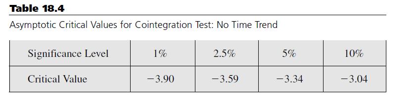
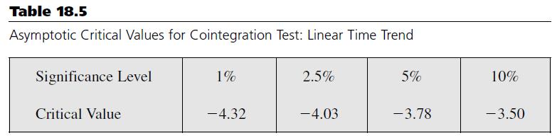
75 Cointegration I In some cases, the integrated series indeed have a close relationship where they share the same stochastic trend. I Suppose y t x 0 t β I (0) that means the error series is indeed stationary, then y t, x t are cointegrated. I In this case, the relationship and the β coe cients can be meaningful. (e.g. long run equilibrium relation.) I The most straightforward way to obtain β is by OLS, then test whether we can reject the unit root for the residual e t = y t xtb. 0 I But the critical values are di erent from the usual DF tests, so you should compare with the critical value of Engle-Granger ADF test. I There are better ways to nd cointegration vector and perform cointegration tests. They are beyond the scope of this brief introduction. 75 / 82

76 Cointegration 76 / 82

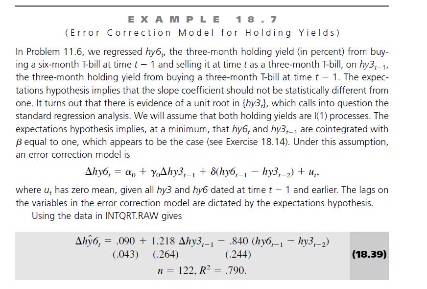
77 Error Correction Model I If variables are cointegrated, we may also add this information to the dynamic model of rst di erenced stationary variables. I In particular, y t = α 0 + q s=0 α 1s x t s + p j=0 α 2j y t j + δ(y t 1 x 0 t 1b) + u t so y t xtb 0 is the deviation from the long-run equilibrium, and the adjustment next period is likely to make the gap smaller. Thus, we would expect that 1 δ 0. I Notice that all variables in the equation are stationary. I This is known as the error correction model (ECM) and the term is error correction term. I Here, though b is estimated, we do not need to adjust for standard errors. Just add this extra variable into the equation. I Again, there are more advanced methods for estimating ECM models, but they are beyond the scope of this introduction. 77 / 82

78 . reg lng_pop lnpg lny_pop t Source SS df MS Number of obs = 52 F( 3, 48) = Model Prob > F = Residual R squared = Adj R squared = Total Root MSE = lng_pop Coef. Std. Err. t P> t [95% Conf. Interval] lnpg lny_pop t _cons predict ub, res. dfuller ub, lag(4) regress Augmented Dickey Fuller test for unit root Number of obs = 47 Interpolated Dickey Fuller Test 1% Critical 5% Critical 10% Critical Statistic Value Value Value Z(t) MacKinnon approximate p value for Z(t) = D.ub Coef. Std. Err. t P> t [95% Conf. Interval] ub L LD L2D L3D L4D _cons / 82

79 Using a user-written SSC command.. egranger lng_pop lnpg lny_pop, regress trend lag(4) Augmented Engle Granger test for cointegration N (1st step) = 52 Number of lags = 4 N (test) = 47 1st step includes linear trend Z(t) Critical values from MacKinnon (1990, 2010) Engle Granger 1st step regression lng_pop Coef. Std. Err. t P> t [95% Conf. Interval] lnpg lny_pop _trend _cons Engle Granger test regression Test 1% Critical 5% Critical 10% Critical Statistic Value Value Value D._egresid Coef. Std. Err. t P> t [95% Conf. Interval] _egresid L LD L2D L3D L4D / 82

80 Suppose we have a cointegrating relation (may be we reject due to weak power), we may look at the ECM model.. *suppose there is a cointegrating relationship (power of test may be bad). *consider the one with trend. reg dlng_pop l(1).dlng_pop dlnpg dlny_pop l.ub Source SS df MS Number of obs = 50 F( 4, 45) = Model Prob > F = Residual R squared = Adj R squared = Total Root MSE = dlng_pop Coef. Std. Err. t P> t [95% Conf. Interval] dlng_pop L dlnpg dlny_pop ub L _cons / 82

81 81 / 82