Week 11 Heteroskedasticity and Autocorrelation
|
|
|
- Poppy Clark
- 5 years ago
- Views:
Transcription
1 Week 11 Heteroskedasticity and Autocorrelation İnsan TUNALI Econ 511 Econometrics I Koç University 27 November 2018
2 Lecture outline 1. OLS and assumptions on V(ε) 2. Violations of V(ε) σ 2 I: 1. Heteroskedasticity 2. Autocorrelation 3. Clustering 3. What to do? Under cases 1 and 2 we examine: 1. Computation and use of robust standard errors 2. Tests for detection of violations 3. Deriving an alternate estimator 4. How inference is affected 5. Model misspecification Draws on: Marno Verbeek, A Guide to Modern Econometrics, 2012 (4 th Ed.), Ch. 4. 2
3 CLRM and OLS Data: (y, X). Rows (y i, x i ) are i.i.d draws from a population which satisfies: (A0) y i = x i β + ε i, i = 1,2,..,N. (A1) Errors have mean zero: E{ε i } = 0 for all i. (A2) ε is independent of X or {ε i, ε N } is independent of {x 1, x N }. All error terms are independent of all explanatory variables. (A3) (A4) V{ε i } = σ 2 for all i. All error terms have the same variance (homoskedasticity). cov{ε i,,ε j } = 0, i j. All error terms are uncorrelated with all other error terms (no autocorrelation). 3
4 OLS estimator properties Under assumptions (A1) and (A2): 1. The OLS estimator b = (X X) -1 X y is unbiased. That is, E{b} = β. Under assumptions (A1), (A2), (A3) and (A4): 2. The variance of the OLS estimator is given by V{b X} = σ 2 (X X) -1 = σ 2 ( Σ i x i x i ) -1 (2.33) nn. where Σ ii Σ ii=1 3. An unbiased estimator for V{b X} may be formed by replacing σ 2 by its unbiased estimator s 2 = (n-k) -1 Σ i e 2 i (2.35) VV {bb XX} = ss 2 (XXXXX) 1 (2.36) 4
5 Gauss-Markov conditions 4. GM Theorem: The OLS estimator b is the best linear unbiased estimator (BLUE) for β. Denoting the N-dimensional vector of all error terms by ε, and the entire matrix of explanatory variables by X, sufficient conditions for the Gauss-Markov results are: E{ ε X} = 0 (4.3) and V{ε X} = σ 2 I, (4.4) where I is the NxN identity matrix. This says: the distribution of error terms given X has zero means, constant variances, and zero covariances. 5
6 Violation of A3: heteroskedasticity Heteroskedasticity arises if error terms do not have the same variance. Relevant to CS, TS and Panel data. How this might happen: TS/Panel: Variances evolve over time. Example: y = daily stock returns. General market conditions are likely to influence the variance of returns. CS/Panel: Variances depend upon one or more explanatory variables. Example: y = household income (or total expenditures). At higher income levels, we expect lower expenditures/higher savings on average, but also more variability. 6
7 Violation of A3: heteroskedasticity Source: Stock and Watson, Intro. to Econometrics. 7
8 Violation of A3: heteroskedasticity 8
9 Violation of A4: autocorrelation Autocorrelation arises if error terms are correlated across observations. Autocorrelation is a typical feature of time-series data (in which case it is also known as serial correlation). When do we expect this? Unobserved factors (included in ε) from one period partly carry over to the next. Model is missing seasonal patterns. Model is based on overlapping samples (e.g. quarterly returns observed each month). Model is otherwise misspecified (omitted variable, incorrect dynamics, etc.) 9
10 Positive autocorrelation Demand for ice cream (as a function of income and price index) 10
11 Positive autocorrelation Demand for Money Greene Example 20.1 (p.943): A naive model: 11
12 Violation of A3 & A4: Clustering Sometimes multiple individual observations contained in a cross-section data set are drawn from the same cluster. Examples: Multiple individuals in the same household. Multiple households from the same city. Multiple firms from the same sector, etc. This induces nonzero correlation between different error terms when observations are from the same cluster. In addition clusters might have different variances. 12
13 Consequences The consequences of both problems are similar. As long as (4.3) holds, i.e. E{ ε X} = 0, the OLS estimator is unbiased. However, if (4.4) is violated (V{ε X} σ 2 I), then: OLS is no longer BLUE! Furthermore: The estimator for V{b X} given by (2.36) is not correct! Standard errors routinely calculated by your software (Stata) are incorrect. F-statistics are not correct; R-sq/RSS based tests do not work. 13
14 What to do? Overview Four ways to deal with the problem: 1. Use OLS but compute standard errors correctly; 2. Use an alternative estimator (FGLS); 3. Test for heteroscedasticity/autocorrelation; use the appropriate (OLS or FGLS) estimator; 4. Reconsider the model specification. The first route is the most popular (easiest). When efficiency is desirable, route 2 is followed. The third may require many tests (pre-test bias?). The fourth route is often employed when autocorrelation is detected. 14
15 Solution 1: Use OLS Model: y i = x i β + ε i,, i = 1,2,, n. In matrix notation: y = Xβ + ε We have V{ε X} = Σ; V{y X} = Σ as well. V{b X} = A V{y X} A = A Σ A = (X X) -1 X ΣX (X X) -1. Estimation of V{b X} requires estimation of Σ. 15
16 1 - (Pure) Heteroskedasticy Easier case: When V{ε X} is diagonal, but with different diagonal elements, we have heteroskedasticity but no autocorrelation. In this case assumption (A3) may be replaced by V{ε i X} = σ 2 i, i = 1,2,, N. V{y i X } = σ 2 i as well. Thus Σ is a diagonal matrix, with σ 2 i as i th diagonal element. Let x i denote the i th row of X. Then X X = Σ i x i x i and X ΣX = Σ i σ 2 ix i x i. 16
17 Estimation of V(b X) under heteroskedasticy Note the difficulty: With V{ε i X} = σ 2 i, each observation has its own unknown parameter! Key insight: ε 2 i is large when σ 2 i is large; e 2 i is large when ε 2 i is large. Σ i e 2 ix i x i serves as a consistent estimator of Σ i σ 2 ix i x i. We can use this idea to estimate V(b X) consistently. This result is due to Eicker, Huber and White. 17
18 Heteroskedasticity-robust inference The (Eicker-Huber-)White (heteroskedasticity-robust) covariance matrix of the OLS estimator b is: VV WW bb XX) = ( (4.30) We use this formula to compute standard errors rather than the standard one from (2.36) and continue as before with our t-tests. (How about F-tests?) Note: This formula is still appropriate if the errors have a constant variance. Robust the formula is valid for arbitrary heteroskedasticity. 18
19 Heteroskedasticity-robust inference To implement in STATA: include subcommand robust after regress. regress y x1 x2.., robust Actually STATA uses a slightly different version of (4.30): VV RR bb XX) = NN NN KK VV WW bb XX). This is because e 2 i s are biased towards zero (recall the bias correction we used earlier, in estimating σ 2 ). See STATA: help vce_option. Also Greene, For additional reading, you may consult Angrist and Pischke (2009) Mostly Harmless Econometrics, Ch.8. 19
20 Example: Demand for labor We estimate a simple labor demand function for a sample of 569 Belgian firms (from 1996). We seek to explain the variation in labor in terms of variation in wages, output and capital stock. Note that the original variables were rescaled to obtain coefficients in the same order of magnitude. 20
21 Demand for labor: A double-log model n = 569 What do the coefficients measure? Any surprises? How might heteroskedasticity influence the results? 21
22 Demand for labor: A double-log model with robust standard errors Compare with Table 4.3. What changed? Should we conclude that labor demand is inelastic with respect to capital? 22
23 Solution 2: Derive an alternative estimator We know that OLS is BLUE only under the Gauss-Markov conditions. How to find an efficient alternative? 1. Transform the model such that it satisfies the Gauss- Markov assumptions again. 2. Apply OLS to the transformed model. This leads to the generalized least squares (GLS) estimator, which is BLUE. See Week 9: GCR. 3. Transformation often depends upon unknown parameters (that characterize heteroskedasticity and/or autocorrelation). In this case we estimate Σ first; then transform the model. This leads to a Feasible GLS (FGLS) or Estimated GLS (EGLS) estimator, which is approximately BLUE. 23
24 Weighted Least Squares (WLS) estimator With heteroskedasticity we have V{ε i X } = σ 2 i = σ 2 h 2 i. (GCR handout p. 32.) Suppose h i s are known. Then y i /h i = (x i /h i ) β + ε i /h i (4.16) has a homoskedastic error term: V{ε i /h i X } = σ 2. OLS applied to this transformed model yields (4.17) which is a weighted least squares (WLS) estimator. 24
25 Weighted Least Squares (WLS) The weighted least squares estimator is a special least squares estimator where each observation is weighted by (a factor proportional to) the inverse of the error variance. Observations with a higher variance get a lower weight (because they provide less accurate info on β). The resulting estimator is more efficient (more accurate) than OLS. However, it can only be applied if we know h i (we rarely do) or if we can estimate it by making additional restrictive assumptions on the form of h i (it is a good idea to test first). 25
26 Implementation of WLS estimation (example of FGLS) Suppose where z i is a vector of observed variables (typically a subset of x i, excluding the constant). Note that this is an example of V{ε i X } = σ 2 i = σ 2 h 2 i. The functional form h(.) has been chosen so that the variances are never negative, and the homoskedastic case obtains as a special case (when all slopes are zero). 26
27 WLS as FGLS, cont d. Assumed form of heteroskedasticity: To estimate α we run an auxiliary regression where e s denote the OLS residuals and z s variables.. This provides a consistent estimator for α, which can be used transform the model (so that OLS on the transformed model would yield the WLS estimator). The auxiliary regression also provides a test for heteroskedasticity and sets the stage for the third approach: Test and decide whether to use OLS or GLS. 27
28 The Breusch-Pagan test of heteroscedasticity The Breusch-Pagan test investigates whether the error variance is a function of the vector z i. In particular, the alternative hypothesis is (4.36) for some function h(.) with h(0) = 1. The all slopes are zero null corresponds to the homoskedastic case. The BP test is based on regressing the squared OLS residuals e 2 i upon z i. Often the original regressors serve as z i. Test statistic ("LM ") = N multiplied by R-sq of the auxiliary regression. Has a Chi-squared distribution (df = no. of variables in z i ). 28
29 A linear model of labor demand Is the variance of labor (level of employment) constant? Or is it likely to vary with covariates? Which ones? 29
30 Breusch-Pagan test Demand for labor example n =
31 The Breusch-Pagan test Demand for labor example cont d. In the auxiliary regression we see (very) high t-ratios and a high R-sq. This indicates that the squared errors are strongly related to z i. Test statistic: LM = NxR-sq ~ Chi Sq (3), here LM o = 331.0, which leads to a very strong rejection of the null hypothesis of homoskedasticity. Example of Lagrange Multiplier test (subject of Week 12) Recall Verbeek s point that using logs reduces heteroscedasticity (Ch.3, section 3.6.2). Results from the double log model reported on the next page lend credence to this. 31
32 A double-log model of labor demand Auxiliary regression (not shown) yields R-sq = ; LM o = NxR-sq = 7.74, p-value n =
33 The White test for heteroscedasticity The White test uses a more general h(.), that is a more general alternative than Breusch-Pagan. It is based on regressing the squared OLS residuals upon all the regressors, their squares and their (unique) cross-products. Test statistic: N multiplied by R 2 of the auxiliary regression. Has Chi-squared distribution (df = no. of variables in the auxiliary regression). Advantage: very general. Disadvantage: low power in small samples (why?). 33
34 The White test Demand for labor example cont d. Verbeek carried out the White test using the double-log model, which is arguably a better functional form choice in this context. The starting point for the investigation is Table 4.3. The auxiliary regression results are given in Table 4.4 (next page). With an R 2 of , the value of the White test statistic is W o = 58.5 (df = 9), a highly significant Chisquared value. 34
35 The White test Demand for labor example n =
36 FGLS Given the strong rejection, the next step would be to turn to WLS (FGLS). Theory: Next page. Results: Verbeek 4.5, Tables Table 4.6: Auxiliary regression (not in lecture notes) Table 4.7: FGLS (or Estimated GLS = EGLS) results 36
37 Multiplicative heteroskedasticity Demand for labor example -- FGLS To obtain the FGLS estimator, compute and transform all observations to obtain The error term in this model is (approximately) homoskedastic. Applying OLS to the transformed model gives the FGLS (Verbeek: EGLS) estimator for β. Note: the transformed regression is for computational purposes only. All economic interpretations refer to the original model! 37
38 38
39 Comparison of Tables 4.5 and 4.7 We see that the efficiency gain is substantial. Comparison with Table 4.3 (OLS with incorrect standard errors) is not appropriate. The coefficient estimates are fairly close to the OLS ones. Note that the effect of capital is now statistically significant. Employment elasticity with respect to capital is indeed negative, but small in absolute magnitude. The R 2 in Table 4.7 is misleading, because - it applies to the transformed model (not the original one); - is uncentered because there is no intercept. Recall that OLS always gives the highest R 2! 39
40 About heteroskedascity robust standard errors RECAP: Use of (Ecker-Huber-)White (heteroskedasticityconsistent) standard errors is often an appropriate solution to the problem of heteroskedasticity. They are easily available in most modern software (such as STATA). It allows one to make appropriate inference without specifying the type of heteroskedasticity. This is (almost) standard in many applications. Sometimes, we would like to have a more efficient estimator, by making some assumption about the form of heteroskedasticity. 40
41 2 - Autocorrelation Autocorrelation typically occurs with time series data (where observations have a natural ordering). To stress this, we shall index the observations by t = 1,,T, rather than i = 1,..,N. The error term picks up the influence of those (many) variables and factors not included in the model. If there is some persistence in these factors, (positive) autocorrelation may arise. Thus, autocorrelation may be an indication of a misspecified model (omitted variables, incorrect functional form, incorrect representation of dynamics). Accordingly, autocorrelation tests are often interpreted as misspecification tests. 41
42 What to do? Four ways to deal with the problem: 1. Use OLS but compute standard errors correctly; 2. Use an alternative estimator (FGLS); 3. Test for autocorrelation; use the appropriate (OLS or FGLS) estimator; 4. Reconsider the model specification. The first route is the most popular. When efficiency is desirable, route 2 is followed. The third may require many tests (pre-test bias?). The fourth route is followed often. 42
43 Solution 1: Use OLS Model: y i = x i β + ε i,, i = 1,2,, n. In matrix notation: y = Xβ + ε We have V{ε X} = Σ; V{y X} = Σ as well. V{b X} = A V{y X} A = A Σ A = (X X) -1 X ΣX (X X) -1. Estimation of V{b X} requires estimation of Σ. 43
44 Estimation of V(b X) under heteroskedasticy and autocorrelation When autocorrelation is present, Σ is no longer diagonal. In this case (A3)-(A4) may be replaced by Cov{ε t ε s X} = σ ts, t, s = 1,2,, T; Cov{y t y s X } = σ ts, t, s = 1,2,, T, as well. The subscripts (t,s) keep track of time, which has a natural ordering. The sample size is denoted by T and σ tt = σ 2 t =V {ε t X}, t = 1,2,, T. TS data typically violate the strong assumption that GMtheorem requires. We settle for consistency instead. (A2) may be replaced by: E(x t ε t ) = 0 for all t. 44
45 Estimation of V(b X) under heteroskedasticy and autocorrelation, cont d. Let x t denote the t th row of X. Then X X = Σ t x t x t and X ΣX = Σ t Σ s σ ts x t x s. Following the key idea of the heteroskedastic case, we might consider estimating X ΣX by Σ t Σ s e t e s x t x s, where e s denote the OLS residuals. Unfortunately this approach has T 2 terms. It is clear that consistency cannot be attained. We have a harder problem at hand, we need simplifying assumptions. 45
46 Estimation of V(b X) under heteroskedasticy and autocorrelation, cont d. Simplification: Suppose V{ε X} is not diagonal, but the error term has certain features: (A2) E(x t ε t ) = 0, (A1) E(ε t ) = 0, for all t; (A3-A4) Cov(ε t ε s ) may be nonzero for t s, but Cov(ε t ε s ) = E(ε t ε s ) = 0 for t s > H > 1. i.e. autocorrelation dies out at lag H. In this case a consistent estimator of V{b X} which is robust to both heteroskedasticity and autocorrelation can be found. The result is due to Newey and West. 46
47 Estimation of V(b X) under heteroskedasticy and autocorrelation, cont d. A consistent estimator of X ΣX is: (4.63) As usual e s denote the OLS residuals. T denotes the sample size. H denotes the lag length at which serial correlation is assumed to become zero. Observe that we obtain the (Huber-Eicker-)White version when w j = 0 for all j. 47
48 Heteroscedasticity and Autocorrelationrobust inference The HAC (heteroskedasticity and autocorrelation- robust) or Newey-West estimator of the covariance matrix of the OLS estimator b is: (4.62) where S* is given in (4.63) on the previous page. The resulting standard errors are known as HAC standard errors or Newey-West standard errors. Special case: When w j = 1 in (4.63), the std. errors are known as Hansen-White standard errors; see Verbeek p
49 Heteroscedasticity and Autocorrelationrobust inference, cont d. STATA implementation: Computation of HAC standard errors (and correct F-stats) is more complicated than heteroskedasticity-consistent inference. Unlike CS data, with TS data correct ordering of the observations is essential. This is facilitated by teaching STATA the time series nature of the data and the variable responsible for the ordering. To get an introduction to STATA s TS commands, type help time series 49
50 About HAC standard errors In many cases, using Newy-West (or Hansen-White) (heteroskedasticity-and-autocorrelation consistent) standard errors is an appropriate solution to the problems that arise with stationary time series data. STATA handles these; read the documentation before you engage in serious work. STATA allows lag length H to be chosen by the researcher. How to choose it? Follow those before you. What to do when the series are non-stationary? Econ 513 (TS version). 50
51 Solutions 2 and 3 -- Overview 2. Use an alternative estimator (FGLS); 3. Test for autocorrelation; use the appropriate (OLS or FGLS) estimator. These require modelling of the errors. Some popular models: AR(1) model: where v t is an error with mean zero and constant variance. MA(1) model: with v t defined in similar fashion. 51
52 Consider First-order autocorrelation Suppose (A1)-(A3) hold, but (A4) is violated. Many forms of autocorrelation exist. The most popular one is first-order autocorrelation: where v t is an error with mean zero and constant variance. GM conditions are restored if ρ = 0. Also known as AR(1): Autoregressive Model of order 1. 52
53 AR(1) -- Properties of ε t We examine the properties of ε t under: ρ < 1 (ρ = 1 case, known as unit roots, is ignored). Covariance stationarity: Means, variances, covariances do not change over time. See Verbeek Ch. 8, Greene Ch. 21 for violations. Under (covariance) stationarity: We can solve for: Note that this requires -1 < ρ < 1. 53
54 First-order autocorrelation Properties of ε t cont d. Further and and in general (s > 0). See GCR handout, Week 9, last page. 54
55 First-order autocorrelation Thus, this form of autocorrelation implies that all error terms are correlated. Their covariance decreases if the distance in time gets large. To transform the model such that it satisfies the Gauss- Markov conditions we use (4.46): With known ρ, this produces (almost) the GLS estimator. Note: first observation is lost by this transformation (see (4.47) on how to handle this). Of course, typically ρ is unknown. 55
56 First-order autocorrelation Estimating ρ First estimate the original model by OLS. This gives the OLS residuals. Starting from it seems natural to estimate ρ by regressing the OLS residual e t upon its lag e t-1. This gives (4.49) We then use (4.49) in (4.46), and apply OLS to the transformed model to get the FGLS estimator. While this estimator is typically biased, it is consistent for ρ under weak conditions. 56
57 Testing for first-order auto-correlation 1. Asymptotic tests The auxiliary regression producing also provides a standard error to it. The resulting t-test statistic is approximately equal to We reject the null (no autocorrelation) against the alternative of nonzero autocorrelation if t > 1.96 (5% significance). Another form is based on (T-1) x R 2 of this regression, to be compared with Chi-squared distribution with df = 1 (reject if > 3.86; 5% significance). 57
58 Testing for first-order auto-correlation 1. Asymptotic tests Remarks: If the model of interest contains lagged values of y t as explanatory variables (or other explanatory variables in lagged form that may be correlated with lagged error terms), the auxiliary regression should also include all explanatory variables. If we also suspect heteroskedasticity, White standard errors may be used in the auxiliary regression. 58
59 Testing for first-order auto-correlation 2. Durbin-Watson test This is a very popular test, routinely computed by most regression packages (even when it is inappropriate!). Requirements: (a) intercept in the model, and (b) no lagged dependent variables! The test statistic is given by which is approximately equal to 59
60 Testing for first-order auto-correlation 2. Durbin-Watson test Distribution is peculiar. It depends on x t s. In general, dw values close to 2 are fine, while dw values close to 0 imply positive autocorrelation. The exact critical value is unknown, but upper and lower bounds can be derived (for extremely slow and fast changing x s --see Table 4.8). Thus (to test for positive autocorrelation): dw is less than lower bound: reject dw is larger than upper bound: not reject dw is in between: inconclusive. The inconclusive region becomes smaller if T gets large. 60
61 Bounds on critical values Durbin-Watson test The test is inconclusive if d L < dw < d U. Conservative approach: Reject null when dw < d U. 61
62 Example: the demand for ice cream Based on classic article Hildreth and Lu (1960), based on a time-series of 30 (!) four-weekly observations See Figure 4.3 for plots of these series. 62
63 The demand for ice cream Figure
64 The demand for ice cream OLS results Note: A simpler model (w/o income) was used to obtain the fitted values in Fig
65 The demand for ice cream Actual and fitted values Based on the OLS results in Table
66 Estimation of ρ From we get = Regressing the OLS residuals on their lags gives. This gives test statistics: Both reject the null of no autocorrelation. Use FGLS or change model specification. 66
67 The demand for ice cream FGLS estimation Compare with Table 4.9. The starred statistics are for the transformed OLS model. New dw-stat is still low! 67
68 The demand for ice cream Augmented model with lagged temperature The new dw-stat is in the inconclusive region.. 68
69 Consider Alternative autocorrelation patterns with first order (autoregressive) autocorrelation This implies that all errors are correlated with each other, with correlations becoming smaller if they are further apart. Two more general alternatives: 1. Higher order autoregression; or 2. Moving average terms. 69
70 Higher order autocorrelation With quarterly or monthly (macro) data, higher order patterns are possible (due to a periodic effect). For example, with quarterly data: or, more generally known as 4 th order (autoregressive) autocorrelation. Correlations between different error terms are more flexible than with 1 st order. 70
71 Moving average autocorrelation Arises if the correlation between different error terms is limited by a maximum time lag. Simplest case: MA(1) Moving Average of order 1. This implies that ε t is correlated with ε t-1, but not with ε t-2 or ε t-3, etc. Moving average errors arise by construction when overlapping samples are used (see Illustration in Section 4.11). 71
72 What to do when you find autocorrelation Autocorrelation may be due to misspecification! 1. Reconsider the model: 1.a: change functional form (e.g. use log(x) rather than x), see Figure 4.5 (on next page). 1.b: extend the model by including additional explanatory variables (seasonals) or additional lags; 2. Compute heteroskedasticity-and-autocorrelation consistent standard errors (HAC standard errors) for the OLS estimator; 3. If you can defend your model, use FGLS. 72
73 Wrong functional form True model: y t = β0 + β1 log(x t ) + ε t We regressed y on x. 73
74 Incomplete dynamics We have been considering the static model y t = x t β + ε t which has E{y t x t } = x t β, with ε t = ρε t-1 + v t. Consider the dynamic alternative (write static model for period t-1, solve for ε t-1 and substitute): E{y t x t, x t-1, y t-1 } = x t β + ρ (y t-1 x t-1 β). Accordingly, we can also write the linear model y t = x t β + ρ y t-1 ρx t-1 β + v t, where the error term does not exhibit serial correlation. In many cases, including lagged values of y and/or x will eliminate the serial correlation problem. 74
75 3 Clustering Robust Inference If clustered CS data are used, error terms of observations drawn from the same group will be correlated, whileas error terms across groups will be uncorrelated. Error terms of clusters may have different variances. The Newey-West formula (4.63) can be adjusted to take care of this situation (see Verbeek, p.390). STATA: use the cluster subsommand to identify the unique variable that marks the different groups (clusters). regress y x1 x2.., cluster(groupvar) 75
76 Clustering example Greene p
Graduate Econometrics Lecture 4: Heteroskedasticity
 Graduate Econometrics Lecture 4: Heteroskedasticity Department of Economics University of Gothenburg November 30, 2014 1/43 and Autocorrelation Consequences for OLS Estimator Begin from the linear model
Introduction to Econometrics. Heteroskedasticity
 Introduction to Econometrics Introduction Heteroskedasticity When the variance of the errors changes across segments of the population, where the segments are determined by different values for the explanatory
Outline. Nature of the Problem. Nature of the Problem. Basic Econometrics in Transportation. Autocorrelation
 1/30 Outline Basic Econometrics in Transportation Autocorrelation Amir Samimi What is the nature of autocorrelation? What are the theoretical and practical consequences of autocorrelation? Since the assumption
LECTURE 11. Introduction to Econometrics. Autocorrelation
 LECTURE 11 Introduction to Econometrics Autocorrelation November 29, 2016 1 / 24 ON PREVIOUS LECTURES We discussed the specification of a regression equation Specification consists of choosing: 1. correct
Econometrics. Week 4. Fall Institute of Economic Studies Faculty of Social Sciences Charles University in Prague
 Econometrics Week 4 Institute of Economic Studies Faculty of Social Sciences Charles University in Prague Fall 2012 1 / 23 Recommended Reading For the today Serial correlation and heteroskedasticity in
Heteroskedasticity. y i = β 0 + β 1 x 1i + β 2 x 2i β k x ki + e i. where E(e i. ) σ 2, non-constant variance.
 σ 2, non-constant variance.") Heteroskedasticity y i = β + β x i + β x i +... + β k x ki + e i where E(e i ) σ, non-constant variance. Common problem with samples over individuals. ê i e ˆi x k x k AREC-ECON 535 Lec F Suppose y i =
Heteroskedasticity y i = β + β x i + β x i +... + β k x ki + e i where E(e i ) σ, non-constant variance. Common problem with samples over individuals. ê i e ˆi x k x k AREC-ECON 535 Lec F Suppose y i =
AUTOCORRELATION. Phung Thanh Binh
 AUTOCORRELATION Phung Thanh Binh OUTLINE Time series Gauss-Markov conditions The nature of autocorrelation Causes of autocorrelation Consequences of autocorrelation Detecting autocorrelation Remedial measures
LECTURE 10: MORE ON RANDOM PROCESSES
 LECTURE 10: MORE ON RANDOM PROCESSES AND SERIAL CORRELATION 2 Classification of random processes (cont d) stationary vs. non-stationary processes stationary = distribution does not change over time more
Lecture 4: Heteroskedasticity
 Lecture 4: Heteroskedasticity Econometric Methods Warsaw School of Economics (4) Heteroskedasticity 1 / 24 Outline 1 What is heteroskedasticity? 2 Testing for heteroskedasticity White Goldfeld-Quandt Breusch-Pagan
A Guide to Modern Econometric:
 A Guide to Modern Econometric: 4th edition Marno Verbeek Rotterdam School of Management, Erasmus University, Rotterdam B 379887 )WILEY A John Wiley & Sons, Ltd., Publication Contents Preface xiii 1 Introduction
Econometrics. 9) Heteroscedasticity and autocorrelation
 Heteroscedasticity and autocorrelation") 30C00200 Econometrics 9) Heteroscedasticity and autocorrelation Timo Kuosmanen Professor, Ph.D. http://nomepre.net/index.php/timokuosmanen Today s topics Heteroscedasticity Possible causes Testing for
30C00200 Econometrics 9) Heteroscedasticity and autocorrelation Timo Kuosmanen Professor, Ph.D. http://nomepre.net/index.php/timokuosmanen Today s topics Heteroscedasticity Possible causes Testing for
Iris Wang.
 Chapter 10: Multicollinearity Iris Wang iris.wang@kau.se Econometric problems Multicollinearity What does it mean? A high degree of correlation amongst the explanatory variables What are its consequences?
Econometrics - 30C00200
 Econometrics - 30C00200 Lecture 11: Heteroskedasticity Antti Saastamoinen VATT Institute for Economic Research Fall 2015 30C00200 Lecture 11: Heteroskedasticity 12.10.2015 Aalto University School of Business
ECON2228 Notes 10. Christopher F Baum. Boston College Economics. cfb (BC Econ) ECON2228 Notes / 48
 ECON2228 Notes / 48") ECON2228 Notes 10 Christopher F Baum Boston College Economics 2014 2015 cfb (BC Econ) ECON2228 Notes 10 2014 2015 1 / 48 Serial correlation and heteroskedasticity in time series regressions Chapter 12:
ECON2228 Notes 10 Christopher F Baum Boston College Economics 2014 2015 cfb (BC Econ) ECON2228 Notes 10 2014 2015 1 / 48 Serial correlation and heteroskedasticity in time series regressions Chapter 12:
Introductory Econometrics
 Based on the textbook by Wooldridge: : A Modern Approach Robert M. Kunst robert.kunst@univie.ac.at University of Vienna and Institute for Advanced Studies Vienna December 11, 2012 Outline Heteroskedasticity
Heteroskedasticity and Autocorrelation
 Lesson 7 Heteroskedasticity and Autocorrelation Pilar González and Susan Orbe Dpt. Applied Economics III (Econometrics and Statistics) Pilar González and Susan Orbe OCW 2014 Lesson 7. Heteroskedasticity
ECON2228 Notes 10. Christopher F Baum. Boston College Economics. cfb (BC Econ) ECON2228 Notes / 54
 ECON2228 Notes / 54") ECON2228 Notes 10 Christopher F Baum Boston College Economics 2014 2015 cfb (BC Econ) ECON2228 Notes 10 2014 2015 1 / 54 erial correlation and heteroskedasticity in time series regressions Chapter 12:
ECON2228 Notes 10 Christopher F Baum Boston College Economics 2014 2015 cfb (BC Econ) ECON2228 Notes 10 2014 2015 1 / 54 erial correlation and heteroskedasticity in time series regressions Chapter 12:
Multiple Regression Analysis
 Multiple Regression Analysis y = 0 + 1 x 1 + x +... k x k + u 6. Heteroskedasticity What is Heteroskedasticity?! Recall the assumption of homoskedasticity implied that conditional on the explanatory variables,
Autocorrelation. Think of autocorrelation as signifying a systematic relationship between the residuals measured at different points in time
 Autocorrelation Given the model Y t = b 0 + b 1 X t + u t Think of autocorrelation as signifying a systematic relationship between the residuals measured at different points in time This could be caused
FinQuiz Notes
 Reading 10 Multiple Regression and Issues in Regression Analysis 2. MULTIPLE LINEAR REGRESSION Multiple linear regression is a method used to model the linear relationship between a dependent variable
Making sense of Econometrics: Basics
 Making sense of Econometrics: Basics Lecture 4: Qualitative influences and Heteroskedasticity Egypt Scholars Economic Society November 1, 2014 Assignment & feedback enter classroom at http://b.socrative.com/login/student/
Wooldridge, Introductory Econometrics, 4th ed. Chapter 15: Instrumental variables and two stage least squares
 Wooldridge, Introductory Econometrics, 4th ed. Chapter 15: Instrumental variables and two stage least squares Many economic models involve endogeneity: that is, a theoretical relationship does not fit
Intermediate Econometrics
 Intermediate Econometrics Heteroskedasticity Text: Wooldridge, 8 July 17, 2011 Heteroskedasticity Assumption of homoskedasticity, Var(u i x i1,..., x ik ) = E(u 2 i x i1,..., x ik ) = σ 2. That is, the
Economics 308: Econometrics Professor Moody
 Economics 308: Econometrics Professor Moody References on reserve: Text Moody, Basic Econometrics with Stata (BES) Pindyck and Rubinfeld, Econometric Models and Economic Forecasts (PR) Wooldridge, Jeffrey
Heteroskedasticity. Part VII. Heteroskedasticity
 Part VII Heteroskedasticity As of Oct 15, 2015 1 Heteroskedasticity Consequences Heteroskedasticity-robust inference Testing for Heteroskedasticity Weighted Least Squares (WLS) Feasible generalized Least
Econ 510 B. Brown Spring 2014 Final Exam Answers
 Econ 510 B. Brown Spring 2014 Final Exam Answers Answer five of the following questions. You must answer question 7. The question are weighted equally. You have 2.5 hours. You may use a calculator. Brevity
the error term could vary over the observations, in ways that are related
 Heteroskedasticity We now consider the implications of relaxing the assumption that the conditional variance Var(u i x i ) = σ 2 is common to all observations i = 1,..., n In many applications, we may
Freeing up the Classical Assumptions. () Introductory Econometrics: Topic 5 1 / 94
 Introductory Econometrics: Topic 5 1 / 94") Freeing up the Classical Assumptions () Introductory Econometrics: Topic 5 1 / 94 The Multiple Regression Model: Freeing Up the Classical Assumptions Some or all of classical assumptions needed for derivations
Freeing up the Classical Assumptions () Introductory Econometrics: Topic 5 1 / 94 The Multiple Regression Model: Freeing Up the Classical Assumptions Some or all of classical assumptions needed for derivations
Model Mis-specification
 Model Mis-specification Carlo Favero Favero () Model Mis-specification 1 / 28 Model Mis-specification Each specification can be interpreted of the result of a reduction process, what happens if the reduction
Reliability of inference (1 of 2 lectures)
") Reliability of inference (1 of 2 lectures) Ragnar Nymoen University of Oslo 5 March 2013 1 / 19 This lecture (#13 and 14): I The optimality of the OLS estimators and tests depend on the assumptions of
Reliability of inference (1 of 2 lectures) Ragnar Nymoen University of Oslo 5 March 2013 1 / 19 This lecture (#13 and 14): I The optimality of the OLS estimators and tests depend on the assumptions of
Heteroskedasticity ECONOMETRICS (ECON 360) BEN VAN KAMMEN, PHD
 BEN VAN KAMMEN, PHD") Heteroskedasticity ECONOMETRICS (ECON 360) BEN VAN KAMMEN, PHD Introduction For pedagogical reasons, OLS is presented initially under strong simplifying assumptions. One of these is homoskedastic errors,
Heteroskedasticity ECONOMETRICS (ECON 360) BEN VAN KAMMEN, PHD Introduction For pedagogical reasons, OLS is presented initially under strong simplifying assumptions. One of these is homoskedastic errors,
Linear Regression with Time Series Data
 Econometrics 2 Linear Regression with Time Series Data Heino Bohn Nielsen 1of21 Outline (1) The linear regression model, identification and estimation. (2) Assumptions and results: (a) Consistency. (b)
ECON3327: Financial Econometrics, Spring 2016
 ECON3327: Financial Econometrics, Spring 2016 Wooldridge, Introductory Econometrics (5th ed, 2012) Chapter 11: OLS with time series data Stationary and weakly dependent time series The notion of a stationary
1 The Multiple Regression Model: Freeing Up the Classical Assumptions
 1 The Multiple Regression Model: Freeing Up the Classical Assumptions Some or all of classical assumptions were crucial for many of the derivations of the previous chapters. Derivation of the OLS estimator
Heteroskedasticity. We now consider the implications of relaxing the assumption that the conditional
 Heteroskedasticity We now consider the implications of relaxing the assumption that the conditional variance V (u i x i ) = σ 2 is common to all observations i = 1,..., In many applications, we may suspect
Multiple Regression Analysis: Heteroskedasticity
 Multiple Regression Analysis: Heteroskedasticity y = β 0 + β 1 x 1 + β x +... β k x k + u Read chapter 8. EE45 -Chaiyuth Punyasavatsut 1 topics 8.1 Heteroskedasticity and OLS 8. Robust estimation 8.3 Testing
Applied Econometrics. Applied Econometrics. Applied Econometrics. Applied Econometrics. What is Autocorrelation. Applied Econometrics
 Autocorrelation 1. What is 2. What causes 3. First and higher orders 4. Consequences of 5. Detecting 6. Resolving Learning Objectives 1. Understand meaning of in the CLRM 2. What causes 3. Distinguish
A Course in Applied Econometrics Lecture 7: Cluster Sampling. Jeff Wooldridge IRP Lectures, UW Madison, August 2008
 A Course in Applied Econometrics Lecture 7: Cluster Sampling Jeff Wooldridge IRP Lectures, UW Madison, August 2008 1. The Linear Model with Cluster Effects 2. Estimation with a Small Number of roups and
MULTIPLE REGRESSION AND ISSUES IN REGRESSION ANALYSIS
 MULTIPLE REGRESSION AND ISSUES IN REGRESSION ANALYSIS Page 1 MSR = Mean Regression Sum of Squares MSE = Mean Squared Error RSS = Regression Sum of Squares SSE = Sum of Squared Errors/Residuals α = Level
Recent Advances in the Field of Trade Theory and Policy Analysis Using Micro-Level Data
 Recent Advances in the Field of Trade Theory and Policy Analysis Using Micro-Level Data July 2012 Bangkok, Thailand Cosimo Beverelli (World Trade Organization) 1 Content a) Classical regression model b)
Applied Econometrics (MSc.) Lecture 3 Instrumental Variables
 Lecture 3 Instrumental Variables") Applied Econometrics (MSc.) Lecture 3 Instrumental Variables Estimation - Theory Department of Economics University of Gothenburg December 4, 2014 1/28 Why IV estimation? So far, in OLS, we assumed independence.
Applied Econometrics (MSc.) Lecture 3 Instrumental Variables Estimation - Theory Department of Economics University of Gothenburg December 4, 2014 1/28 Why IV estimation? So far, in OLS, we assumed independence.
Applied Microeconometrics (L5): Panel Data-Basics
: Panel Data-Basics") Applied Microeconometrics (L5): Panel Data-Basics Nicholas Giannakopoulos University of Patras Department of Economics ngias@upatras.gr November 10, 2015 Nicholas Giannakopoulos (UPatras) MSc Applied Economics
Applied Microeconometrics (L5): Panel Data-Basics Nicholas Giannakopoulos University of Patras Department of Economics ngias@upatras.gr November 10, 2015 Nicholas Giannakopoulos (UPatras) MSc Applied Economics
CHAPTER 6: SPECIFICATION VARIABLES
 Recall, we had the following six assumptions required for the Gauss-Markov Theorem: 1. The regression model is linear, correctly specified, and has an additive error term. 2. The error term has a zero
Topic 7: Heteroskedasticity
 Topic 7: Heteroskedasticity Advanced Econometrics (I Dong Chen School of Economics, Peking University Introduction If the disturbance variance is not constant across observations, the regression is heteroskedastic
13. Time Series Analysis: Asymptotics Weakly Dependent and Random Walk Process. Strict Exogeneity
 Outline: Further Issues in Using OLS with Time Series Data 13. Time Series Analysis: Asymptotics Weakly Dependent and Random Walk Process I. Stationary and Weakly Dependent Time Series III. Highly Persistent
Econometrics Honor s Exam Review Session. Spring 2012 Eunice Han
 Econometrics Honor s Exam Review Session Spring 2012 Eunice Han Topics 1. OLS The Assumptions Omitted Variable Bias Conditional Mean Independence Hypothesis Testing and Confidence Intervals Homoskedasticity
Wooldridge, Introductory Econometrics, 2d ed. Chapter 8: Heteroskedasticity In laying out the standard regression model, we made the assumption of
 Wooldridge, Introductory Econometrics, d ed. Chapter 8: Heteroskedasticity In laying out the standard regression model, we made the assumption of homoskedasticity of the regression error term: that its
Econometrics. Week 8. Fall Institute of Economic Studies Faculty of Social Sciences Charles University in Prague
 Econometrics Week 8 Institute of Economic Studies Faculty of Social Sciences Charles University in Prague Fall 2012 1 / 25 Recommended Reading For the today Instrumental Variables Estimation and Two Stage
1. You have data on years of work experience, EXPER, its square, EXPER2, years of education, EDUC, and the log of hourly wages, LWAGE
 1. You have data on years of work experience, EXPER, its square, EXPER, years of education, EDUC, and the log of hourly wages, LWAGE You estimate the following regressions: (1) LWAGE =.00 + 0.05*EDUC +
Instrumental Variables, Simultaneous and Systems of Equations
 Chapter 6 Instrumental Variables, Simultaneous and Systems of Equations 61 Instrumental variables In the linear regression model y i = x iβ + ε i (61) we have been assuming that bf x i and ε i are uncorrelated
ECON 4230 Intermediate Econometric Theory Exam
 ECON 4230 Intermediate Econometric Theory Exam Multiple Choice (20 pts). Circle the best answer. 1. The Classical assumption of mean zero errors is satisfied if the regression model a) is linear in the
Heteroscedasticity and Autocorrelation
 Heteroscedasticity and Autocorrelation Carlo Favero Favero () Heteroscedasticity and Autocorrelation 1 / 17 Heteroscedasticity, Autocorrelation, and the GLS estimator Let us reconsider the single equation
1 Motivation for Instrumental Variable (IV) Regression
 Regression") ECON 370: IV & 2SLS 1 Instrumental Variables Estimation and Two Stage Least Squares Econometric Methods, ECON 370 Let s get back to the thiking in terms of cross sectional (or pooled cross sectional) data
ECON 370: IV & 2SLS 1 Instrumental Variables Estimation and Two Stage Least Squares Econometric Methods, ECON 370 Let s get back to the thiking in terms of cross sectional (or pooled cross sectional) data
Modified Variance Ratio Test for Autocorrelation in the Presence of Heteroskedasticity
 The Lahore Journal of Economics 23 : 1 (Summer 2018): pp. 1 19 Modified Variance Ratio Test for Autocorrelation in the Presence of Heteroskedasticity Sohail Chand * and Nuzhat Aftab ** Abstract Given that
Internal vs. external validity. External validity. This section is based on Stock and Watson s Chapter 9.
 Section 7 Model Assessment This section is based on Stock and Watson s Chapter 9. Internal vs. external validity Internal validity refers to whether the analysis is valid for the population and sample
Lecture 6: Dynamic Models
 Lecture 6: Dynamic Models R.G. Pierse 1 Introduction Up until now we have maintained the assumption that X values are fixed in repeated sampling (A4) In this lecture we look at dynamic models, where the
Semester 2, 2015/2016
 ECN 3202 APPLIED ECONOMETRICS 5. HETEROSKEDASTICITY Mr. Sydney Armstrong Lecturer 1 The University of Guyana 1 Semester 2, 2015/2016 WHAT IS HETEROSKEDASTICITY? The multiple linear regression model can
Econometrics Summary Algebraic and Statistical Preliminaries
 Econometrics Summary Algebraic and Statistical Preliminaries Elasticity: The point elasticity of Y with respect to L is given by α = ( Y/ L)/(Y/L). The arc elasticity is given by ( Y/ L)/(Y/L), when L
Econ 300/QAC 201: Quantitative Methods in Economics/Applied Data Analysis. 17th Class 7/1/10
 Econ 300/QAC 201: Quantitative Methods in Economics/Applied Data Analysis 17th Class 7/1/10 The only function of economic forecasting is to make astrology look respectable. --John Kenneth Galbraith show
Auto correlation 2. Note: In general we can have AR(p) errors which implies p lagged terms in the error structure, i.e.,
 errors which implies p lagged terms in the error structure, i.e.,") 1 Motivation Auto correlation 2 Autocorrelation occurs when what happens today has an impact on what happens tomorrow, and perhaps further into the future This is a phenomena mainly found in time-series
1 Motivation Auto correlation 2 Autocorrelation occurs when what happens today has an impact on what happens tomorrow, and perhaps further into the future This is a phenomena mainly found in time-series
Diagnostics of Linear Regression
 Diagnostics of Linear Regression Junhui Qian October 7, 14 The Objectives After estimating a model, we should always perform diagnostics on the model. In particular, we should check whether the assumptions
Section 6: Heteroskedasticity and Serial Correlation
 From the SelectedWorks of Econ 240B Section February, 2007 Section 6: Heteroskedasticity and Serial Correlation Jeffrey Greenbaum, University of California, Berkeley Available at: https://works.bepress.com/econ_240b_econometrics/14/
Christopher Dougherty London School of Economics and Political Science
 Introduction to Econometrics FIFTH EDITION Christopher Dougherty London School of Economics and Political Science OXFORD UNIVERSITY PRESS Contents INTRODU CTION 1 Why study econometrics? 1 Aim of this
Introduction to Econometrics
 Introduction to Econometrics T H I R D E D I T I O N Global Edition James H. Stock Harvard University Mark W. Watson Princeton University Boston Columbus Indianapolis New York San Francisco Upper Saddle
Econometrics Multiple Regression Analysis: Heteroskedasticity
 Econometrics Multiple Regression Analysis: João Valle e Azevedo Faculdade de Economia Universidade Nova de Lisboa Spring Semester João Valle e Azevedo (FEUNL) Econometrics Lisbon, April 2011 1 / 19 Properties
Answer all questions from part I. Answer two question from part II.a, and one question from part II.b.
 B203: Quantitative Methods Answer all questions from part I. Answer two question from part II.a, and one question from part II.b. Part I: Compulsory Questions. Answer all questions. Each question carries
Reading Assignment. Serial Correlation and Heteroskedasticity. Chapters 12 and 11. Kennedy: Chapter 8. AREC-ECON 535 Lec F1 1
 Reading Assignment Serial Correlation and Heteroskedasticity Chapters 1 and 11. Kennedy: Chapter 8. AREC-ECON 535 Lec F1 1 Serial Correlation or Autocorrelation y t = β 0 + β 1 x 1t + β x t +... + β k
Panel Data Models. Chapter 5. Financial Econometrics. Michael Hauser WS17/18 1 / 63
 1 / 63 Panel Data Models Chapter 5 Financial Econometrics Michael Hauser WS17/18 2 / 63 Content Data structures: Times series, cross sectional, panel data, pooled data Static linear panel data models:
ECONOMETRICS HONOR S EXAM REVIEW SESSION
 ECONOMETRICS HONOR S EXAM REVIEW SESSION Eunice Han ehan@fas.harvard.edu March 26 th, 2013 Harvard University Information 2 Exam: April 3 rd 3-6pm @ Emerson 105 Bring a calculator and extra pens. Notes
Econometrics of Panel Data
 Econometrics of Panel Data Jakub Mućk Meeting # 1 Jakub Mućk Econometrics of Panel Data Meeting # 1 1 / 31 Outline 1 Course outline 2 Panel data Advantages of Panel Data Limitations of Panel Data 3 Pooled
Repeated observations on the same cross-section of individual units. Important advantages relative to pure cross-section data
 Panel data Repeated observations on the same cross-section of individual units. Important advantages relative to pure cross-section data - possible to control for some unobserved heterogeneity - possible
Likely causes: The Problem. E u t 0. E u s u p 0
 Autocorrelation This implies that taking the time series regression Y t X t u t but in this case there is some relation between the error terms across observations. E u t 0 E u t E u s u p 0 Thus the error
Econometrics Part Three
 !1 I. Heteroskedasticity A. Definition 1. The variance of the error term is correlated with one of the explanatory variables 2. Example -- the variance of actual spending around the consumption line increases
Time Series Econometrics For the 21st Century
 Time Series Econometrics For the 21st Century by Bruce E. Hansen Department of Economics University of Wisconsin January 2017 Bruce Hansen (University of Wisconsin) Time Series Econometrics January 2017
F9 F10: Autocorrelation
 F9 F10: Autocorrelation Feng Li Department of Statistics, Stockholm University Introduction In the classic regression model we assume cov(u i, u j x i, x k ) = E(u i, u j ) = 0 What if we break the assumption?
Review of Econometrics
 Review of Econometrics Zheng Tian June 5th, 2017 1 The Essence of the OLS Estimation Multiple regression model involves the models as follows Y i = β 0 + β 1 X 1i + β 2 X 2i + + β k X ki + u i, i = 1,...,
1. The OLS Estimator. 1.1 Population model and notation
 1. The OLS Estimator OLS stands for Ordinary Least Squares. There are 6 assumptions ordinarily made, and the method of fitting a line through data is by least-squares. OLS is a common estimation methodology
Agricultural and Applied Economics 637 Applied Econometrics II
 Agricultural and Applied Economics 637 Applied Econometrics II Assignment 1 Review of GLS Heteroskedasity and Autocorrelation (Due: Feb. 4, 2011) In this assignment you are asked to develop relatively
Chapter 8 Heteroskedasticity
 Chapter 8 Walter R. Paczkowski Rutgers University Page 1 Chapter Contents 8.1 The Nature of 8. Detecting 8.3 -Consistent Standard Errors 8.4 Generalized Least Squares: Known Form of Variance 8.5 Generalized
9. AUTOCORRELATION. [1] Definition of Autocorrelation (AUTO) 1) Model: y t = x t β + ε t. We say that AUTO exists if cov(ε t,ε s ) 0, t s.
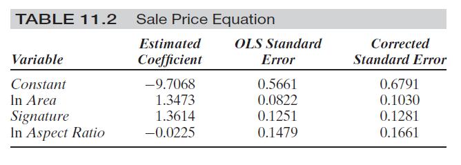
![9. AUTOCORRELATION. [1] Definition of Autocorrelation (AUTO) 1) Model: y t = x t β + ε t. We say that AUTO exists if cov(ε t,ε s ) 0, t s.](/thumbs/91/106709242.jpg "9. AUTOCORRELATION. [1] Definition of Autocorrelation (AUTO) 1) Model: y t = x t β + ε t. We say that AUTO exists if cov(ε t,ε s ) 0, t s.") 9. AUTOCORRELATION [1] Definition of Autocorrelation (AUTO) 1) Model: y t = x t β + ε t. We say that AUTO exists if cov(ε t,ε s ) 0, t s. ) Assumptions: All of SIC except SIC.3 (the random sample assumption).
9. AUTOCORRELATION [1] Definition of Autocorrelation (AUTO) 1) Model: y t = x t β + ε t. We say that AUTO exists if cov(ε t,ε s ) 0, t s. ) Assumptions: All of SIC except SIC.3 (the random sample assumption).
Outline. Possible Reasons. Nature of Heteroscedasticity. Basic Econometrics in Transportation. Heteroscedasticity
 1/25 Outline Basic Econometrics in Transportation Heteroscedasticity What is the nature of heteroscedasticity? What are its consequences? How does one detect it? What are the remedial measures? Amir Samimi
Econometrics I KS. Module 2: Multivariate Linear Regression. Alexander Ahammer. This version: April 16, 2018
 Econometrics I KS Module 2: Multivariate Linear Regression Alexander Ahammer Department of Economics Johannes Kepler University of Linz This version: April 16, 2018 Alexander Ahammer (JKU) Module 2: Multivariate
Panel Data. March 2, () Applied Economoetrics: Topic 6 March 2, / 43
 Applied Economoetrics: Topic 6 March 2, / 43") Panel Data March 2, 212 () Applied Economoetrics: Topic March 2, 212 1 / 43 Overview Many economic applications involve panel data. Panel data has both cross-sectional and time series aspects. Regression
Panel Data March 2, 212 () Applied Economoetrics: Topic March 2, 212 1 / 43 Overview Many economic applications involve panel data. Panel data has both cross-sectional and time series aspects. Regression
in the time series. The relation between y and x is contemporaneous.
 9 Regression with Time Series 9.1 Some Basic Concepts Static Models (1) y t = β 0 + β 1 x t + u t t = 1, 2,..., T, where T is the number of observation in the time series. The relation between y and x
Multiple Regression Analysis
 1 OUTLINE Basic Concept: Multiple Regression MULTICOLLINEARITY AUTOCORRELATION HETEROSCEDASTICITY REASEARCH IN FINANCE 2 BASIC CONCEPTS: Multiple Regression Y i = β 1 + β 2 X 1i + β 3 X 2i + β 4 X 3i +
Introduction to Regression Analysis. Dr. Devlina Chatterjee 11 th August, 2017
 Introduction to Regression Analysis Dr. Devlina Chatterjee 11 th August, 2017 What is regression analysis? Regression analysis is a statistical technique for studying linear relationships. One dependent
11.1 Gujarati(2003): Chapter 12
: Chapter 12") 11.1 Gujarati(2003): Chapter 12 Time Series Data 11.2 Time series process of economic variables e.g., GDP, M1, interest rate, echange rate, imports, eports, inflation rate, etc. Realization An observed
11.1 Gujarati(2003): Chapter 12 Time Series Data 11.2 Time series process of economic variables e.g., GDP, M1, interest rate, echange rate, imports, eports, inflation rate, etc. Realization An observed
Eksamen på Økonomistudiet 2006-II Econometrics 2 June 9, 2006
 Eksamen på Økonomistudiet 2006-II Econometrics 2 June 9, 2006 This is a four hours closed-book exam (uden hjælpemidler). Please answer all questions. As a guiding principle the questions 1 to 4 have equal
Panel Data Models. James L. Powell Department of Economics University of California, Berkeley
 Panel Data Models James L. Powell Department of Economics University of California, Berkeley Overview Like Zellner s seemingly unrelated regression models, the dependent and explanatory variables for panel
Ordinary Least Squares Regression
 Ordinary Least Squares Regression Goals for this unit More on notation and terminology OLS scalar versus matrix derivation Some Preliminaries In this class we will be learning to analyze Cross Section
Introductory Econometrics
 Based on the textbook by Wooldridge: : A Modern Approach Robert M. Kunst robert.kunst@univie.ac.at University of Vienna and Institute for Advanced Studies Vienna October 16, 2013 Outline Introduction Simple
Models, Testing, and Correction of Heteroskedasticity. James L. Powell Department of Economics University of California, Berkeley
 Models, Testing, and Correction of Heteroskedasticity James L. Powell Department of Economics University of California, Berkeley Aitken s GLS and Weighted LS The Generalized Classical Regression Model
Econ 836 Final Exam. 2 w N 2 u N 2. 2 v N
 1) [4 points] Let Econ 836 Final Exam Y Xβ+ ε, X w+ u, w N w~ N(, σi ), u N u~ N(, σi ), ε N ε~ Nu ( γσ, I ), where X is a just one column. Let denote the OLS estimator, and define residuals e as e Y X.
Heteroskedasticity. Occurs when the Gauss Markov assumption that the residual variance is constant across all observations in the data set
 Heteroskedasticity Occurs when the Gauss Markov assumption that the residual variance is constant across all observations in the data set Heteroskedasticity Occurs when the Gauss Markov assumption that
Econometrics of Panel Data
 Econometrics of Panel Data Jakub Mućk Meeting # 4 Jakub Mućk Econometrics of Panel Data Meeting # 4 1 / 30 Outline 1 Two-way Error Component Model Fixed effects model Random effects model 2 Non-spherical
Please discuss each of the 3 problems on a separate sheet of paper, not just on a separate page!
 Econometrics - Exam May 11, 2011 1 Exam Please discuss each of the 3 problems on a separate sheet of paper, not just on a separate page! Problem 1: (15 points) A researcher has data for the year 2000 from
Applied Quantitative Methods II
 Applied Quantitative Methods II Lecture 4: OLS and Statistics revision Klára Kaĺıšková Klára Kaĺıšková AQM II - Lecture 4 VŠE, SS 2016/17 1 / 68 Outline 1 Econometric analysis Properties of an estimator
ECON 366: ECONOMETRICS II. SPRING TERM 2005: LAB EXERCISE #10 Nonspherical Errors Continued. Brief Suggested Solutions
 DEPARTMENT OF ECONOMICS UNIVERSITY OF VICTORIA ECON 366: ECONOMETRICS II SPRING TERM 2005: LAB EXERCISE #10 Nonspherical Errors Continued Brief Suggested Solutions 1. In Lab 8 we considered the following
Using EViews Vox Principles of Econometrics, Third Edition
 Using EViews Vox Principles of Econometrics, Third Edition WILLIAM E. GRIFFITHS University of Melbourne R. CARTER HILL Louisiana State University GUAY С LIM University of Melbourne JOHN WILEY & SONS, INC
DEMAND ESTIMATION (PART III)
") BEC 30325: MANAGERIAL ECONOMICS Session 04 DEMAND ESTIMATION (PART III) Dr. Sumudu Perera Session Outline 2 Multiple Regression Model Test the Goodness of Fit Coefficient of Determination F Statistic t
BEC 30325: MANAGERIAL ECONOMICS Session 04 DEMAND ESTIMATION (PART III) Dr. Sumudu Perera Session Outline 2 Multiple Regression Model Test the Goodness of Fit Coefficient of Determination F Statistic t