Econometrics and Structural
|
|
|
- Mary Cunningham
- 5 years ago
- Views:
Transcription
1 Introduction to Time Series Econometrics and Structural Breaks Ziyodullo Parpiev, PhD
2 Outline 1. Stochastic processes 2. Stationary processes 3. Purely random processes 4. Nonstationary processes 5. Integrated variables 6. Random walk models 7. Cointegration 8. Deterministic and stochastic trends 9. Unit root tests
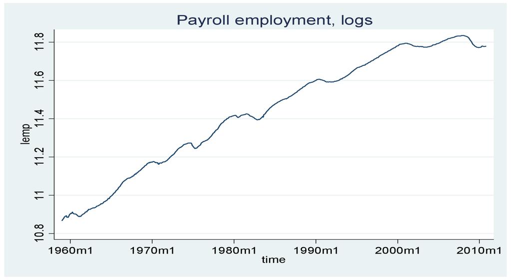
3 What is a time series? A time series is any series of data that varies over time. For example Payroll employment in the U.S. Unemployment rate 12-month inflation rate Daily price of stocks and shares Quarterly GDP series Annual precipitation (rain and snowfall) Because of widespread availability of time series databases most empirical studies use time series data.

4 Some monthly U.S. macro and financial time series
5

6

7

8
9 A daily financial time series:
10 STOCHASTIC PROCESSES A random or stochastic process is a collection of random variables ordered in time. If we let Y denote a random variable, and if it is continuous, we denote it as Y(t), but if it is discrete, we denoted it as Yt. An example of the former is an electrocardiogram, and an example of the latter is GDP, PDI, etc. Since most economic data are collected at discrete points in time, for our purpose we will use the notation Yt rather than Y(t). Keep in mind that each of these Y s is a random variable. In what sense can we regard GDP as a stochastic process? Consider for instance the GDP of $ billion for 1970 I. In theory, the GDP figure for the first quarter of 1970 could have been any number, depending on the economic and political climate then prevailing. The figure of is a particular realization of all such possibilities. The distinction between the stochastic process and its realization is akin to the distinction between population and sample in cross-sectional data.
11 Stationary Stochastic Processes Forms of Stationarity: weak, and strong (i) mean: E(Y t ) = μ (ii) variance: var(y t ) = E( Y t μ) 2 = σ 2 (iii) Covariance: γ k = E[(Y t μ)(y t-k μ) 2 where γk, the covariance (or autocovariance) at lag k, is the covariance between the values of Yt and Yt+k, that is, between two Y values k periods apart. If k = 0, we obtain γ0, which is simply the variance of Y (= σ2); if k = 1, γ1 is the covariance between two adjacent values of Y, the type of covariance we encountered in Chapter 12 (recall the Markov first-order autoregressive scheme).
12 Types of Stationarity A time series is weakly stationary if its mean and variance are constant over time and the value of the covariance between two periods depends only on the distance (or lags) between the two periods. A time series if strongly stationary if for any values j 1, j 2, j n, the joint distribution of (Y t, Y t+j1, Y t+j2, Y t+jn ) depends only on the intervals separating the dates (j 1, j 2,,j n ) and not on the date itself (t). A weakly stationary series that is Gaussian (normal) is also strictly stationary. This is why we often test for the normality of a time series.
13 Stationarity vs. Nonstationarity A time series is stationary, if its mean, variance, and autocovariance (at various lags) remain the same no matter at what point we measure them; that is, they are time invariant. Such a time series will tend to return to its mean (called mean reversion) and fluctuations around this mean (measured by its variance) will have a broadly constant amplitude. If a time series is not stationary in the sense just defined, it is called a nonstationary time series (keep in mind we are talking only about weak stationarity). In other words, a nonstationary time series will have a timevarying mean or a time-varying variance or both. Why are stationary time series so important? Because if a time series is nonstationary, we can study its behavior only for the time period under consideration. Each set of time series data will therefore be for a particular episode. As a consequence, it is not possible to generalize it to other time periods. Therefore, for the purpose of forecasting, such time series may be of little practical value.
14 Examples of Non-Stationary Time Series AU STR ALIA C AN AD A C H IN A GER MAN Y H ON GKON G J APAN KOR EA MALAYSIA SIN GAPOR E TAIW AN UK U SA
15 Examples of Stationary Time Series AU ST C AN CHI GER M H ON G J AP KOR MAL SIN G TW N U KK US
16 Unit Root and order of integration If a Non-Stationary Time Series Y t has to be differenced d times to make it stationary, then Y t is said to contain d Unit Roots. It is customary to denote Y t ~ I(d) which reads Y t is integrated of order d If Y t ~ I(0), then Y t is Stationary If Y t ~ I(1), then Z t = Y t Y t-1 is Stationary If Y t ~ I(2), then Z t = Y t Y t-1 (Y t Y t-2 )is Stationary
17 Unit Roots Consider an AR(1) process: y t = a 1 y t-1 + ε t (Eq. 1) ε t ~ N(0, σ 2 ) Case #1: Random walk (a 1 = 1) y t = y t-1 + ε t Δy t = ε t
18 Unit Roots In this model, the variance of the error term, ε t, increases as t increases, in which case OLS will produce a downwardly biased estimate of a 1 (Hurwicz bias). Rewrite equation 1 by subtracting y t-1 from both sides: y t y t-1 = a 1 y t-1 y t-1 + ε t (Eq. 2) Δy t = δ y t-1 + ε t δ = (a 1 1)
19 Unit Roots H 0 : δ = 0 (there is a unit root) H A : δ 0 (there is not a unit root) If δ = 0, then we can rewrite Equation 2 as Δy t = ε t Thus first differences of a random walk time series are stationary, because by assumption, ε t is purely random. In general, a time series must be differenced d times to become stationary; it is integrated of order d or I(d). A stationary series is I(0). A random walk series is I(1).
20 Tests for Unit Roots Dickey-Fuller test Estimates a regression using equation 2 The usual t-statistic is not valid, thus D-F developed appropriate critical values. You can include a constant, trend, or both in the test. If you accept the null hypothesis, you conclude that the time series has a unit root. In that case, you should first difference the series before proceeding with analysis.
21 Tests for Unit Roots Augmented Dickey-Fuller test (dfuller in STATA) We can use this version if we suspect there is autocorrelation in the residuals. This model is the same as the DF test, but includes lags of the residuals too. Phillips-Perron test (pperron in STATA) Makes milder assumptions concerning the error term, allowing for the ε t to be weakly dependent and heterogenously distributed. Other tests include KPSS test, Variance Ratio test, and Modified Rescaled Range test. There are also unit root tests for panel data (Levin et al 2002, Pesaran et al).
22 Tests for Unit Roots These tests have been criticized for having low power (1-probability(Type II error)). They tend to (falsely) accept H o too often, finding unit roots frequently, especially with seasonally adjusted data or series with structural breaks. Results are also sensitive to # of lags used in the test. Solution involves increasing the frequency of observations, or obtaining longer time series.
23 Trend Stationary vs. Difference Stationary Traditionally in regression-based time series models, a time trend variable, t, was included as one of the regressors to avoid spurious correlation. This practice is only valid if the trend variable is deterministic, not stochastic. A trend stationary series has a data generating process (DGP) of: y t = a 0 + a 1 t + ε t
24 Trend Stationary vs. Difference Stationary A difference stationary time series has a DGP of: y t - y t-1 = a 0 + ε t Δy t = a 0 + ε t Run the ADF test with a trend. If the test still shows a unit root (accept H o ), then conclude it is difference stationary. If you reject H o, you could simply include the time trend in the model.
25 What is a Spurious Regression? A Spurious or Nonsensical relationship may result when one Non-stationary time series is regressed against one or more Non-stationary time series The best way to guard against Spurious Regressions is to check for Cointegration of the variables used in time series modeling
26 Symptoms of Likely Presence of Spurious Regression If the R 2 of the regression is greater than the Durbin-Watson Statistic If the residual series of the regression has a Unit Root
27 Examples of spurious relationships For school children, shoe size is strongly correlated with reading skills. Amount of ice cream sold and death by drowning in monthly data Number of doctors and number of people dying of disease in cities Number of libraries and number of people on drugs in annual data Bottom line: Correlation measures association. But association is not the same as causation. More complicated case: Fat in the diet seems to be correlated with cancer. Can we say the diagram is some evidence for the theory? But the evidence is quite weak, because other things aren't equal. For example, the countries with lots of fat in the diet also have lots of sugar. A plot of colon cancer rates against sugar consumption would look just like figure 8, and nobody thinks that sugar causes colon cancer. As it turns out, fat and sugar are relatively expensive. In rich countries, people can afford to eat fat and sugar rather than starchier grain products. Some aspects of the diet in these countries, or other factors in the life-style, probably do cause certain kinds of cancer and protect against other kinds. So far, epidemiologists can identify only a few of these factors with any real confidence. Fat is not among them
28
29 Cointegration Is the existence of a long run equilibrium relationship among time series variables Is a property of two or more variables moving together through time, and despite following their own individual trends will not drift too far apart since they are linked together in some sense
30
31 Cointegration Analysis: Formal Tests Cointegrating Regression Durbin-Watson (CRDW) Test Augmented Engle-Granger (AEG) Test Johansen Multivariate Cointegration Tests or the Johansen Method
32 Error Correction Mechanism (ECM) Reconciles the Static LR Equilibrium relationship of Cointegrated Time Series with its Dynamic SR disequilibrium Based on the Granger Representation Theorem which states that If variables are cointegrated, the relationship among them can be expressed as ECM.
33 6. Nonstationarity I: Trends So far, we have assumed that the data are stationary, that is, the distribution of (Y s+1,, Y s+t ) doesn t depend on s. If stationarity doesn t hold, the series are said to be nonstationary. Two important types of nonstationarity are: Trends Structural breaks (model instability)
34 Outline of discussion of trends in time series data: A. What is a trend? B. Deterministic and stochastic (random) trends C. How do you detect stochastic trends (statistical tests)?
35 A. What is a trend? A trend is a persistent, long-term movement or tendency in the data. Trends need not be just a straight line! Which of these series has a trend?
36
37
38 What is a trend, ctd. The three series: Log Japan GDP clearly has a long-run trend not a straight line, but a slowly decreasing trend fast growth during the 1960s and 1970s, slower during the 1980s, stagnating during the 1990s/2000s. Inflation has long-term swings, periods in which it is persistently high for many years ( 70s/early 80s) and periods in which it is persistently low. Maybe it has a trend hard to tell. NYSE daily changes has no apparent trend. There are periods of persistently high volatility but this isn t a trend.
39 B. Deterministic and stochastic trends A trend is a long-term movement or tendency in the data. A deterministic trend is a nonrandom function of time (e.g. y t = t, or y t = t 2 ). A stochastic trend is random and varies over time An important example of a stochastic trend is a random walk: Y t = Y t 1 + u t, where u t is serially uncorrelated If Y t follows a random walk, then the value of Y tomorrow is the value of Y today, plus an unpredictable disturbance.
40 Deterministic and stochastic trends, ctd. Two key features of a random walk: (i) Y T+h T = Y T Your best prediction of the value of Y in the future is the value of Y today To a first approximation, log stock prices follow a random walk (more precisely, stock returns are unpredictable) (ii) Suppose Y 0 = 0. Then var(y t ) =. t u 2 This variance depends on t (increases linearly with t), so Y t isn t stationary (recall the definition of stationarity).
41 Deterministic and stochastic trends, ctd. A random walk with drift is Y t = β 0 +Y t 1 + u t, where u t is serially uncorrelated The drift is β 0 : If β 0 0, then Y t follows a random walk around a linear trend. You can see this by considering the h-step ahead forecast: Y T+h T = β 0 h + Y T The random walk model (with or without drift) is a good description of stochastic trends in many economic time series.
42 C. How do you detect stochastic trends? 1. Plot the data are there persistent long-run movements? 2. Use a regression-based test for a random walk: the Dickey-Fuller test for a unit root. The Dickey-Fuller test in an AR(1) or Y t = β 0 + β 1 Y t 1 + u t ΔY t = β 0 + δy t 1 + u t H 0 : δ = 0 (that is, β 1 = 1) v. H 1 : δ < 0 (note: this is 1-sided: δ < 0 means that Y t is stationary)
43 DF test in AR(1), ctd. ΔY t = β 0 + δy t 1 + u t H 0 : δ = 0 (that is, β 1 = 1) v. H 1 : δ < 0 DF test: compute the t-statistic testing δ = 0 Under H 0, this t statistic does not have a normal distribution! You need to use the table of Dickey-Fuller critical values. There are two cases, which have different critical values: (a) ΔY t = β 0 + δy t 1 + u t (intercept only) (b) ΔY t = β 0 + μt + δy t 1 + u t (intercept & time trend)
44 The Dickey-Fuller Test in an AR(p) In an AR(p), the DF test is based on the rewritten model, ΔY t = β 0 + δy t 1 + γ 1 ΔY t 1 + γ 2 ΔY t γ p 1 ΔY t p+1 + u t (*) where δ = β 1 + β β p 1. If there is a unit root (random walk trend), δ = 0; if the AR is stationary, δ < 1. The DF test in an AR(p) (intercept only): 1. Estimate (*), obtain the t-statistic testing δ = 0 2. Reject the null hypothesis of a unit root if the t-statistic is less than the DF critical value
45 When should you include a time trend in the DF test? The decision to use the intercept-only DF test or the intercept & trend DF test depends on what the alternative is and what the data look like. In the intercept-only specification, the alternative is that Y is stationary around a constant no long-term growth in the series In the intercept & trend specification, the alternative is that Y is stationary around a linear time trend the series has long-term growth.
46 Example: Does U.S. inflation have a unit root? The alternative is that inflation is stationary around a constant
47 Does U.S. inflation have a unit root? Ctd DF test for a unit root in U.S. inflation using p = 4 lags. reg dinf L.inf L(1/4).dinf if tin(1962q1,2004q4); Source SS df MS Number of obs = F( 5, 166) = Model Prob > F = Residual R-squared = Adj R-squared = Total Root MSE = dinf Coef. Std. Err. t P> t [95% Conf. Interval] inf L dinf L L L L _cons
 vs. the alternative that the autoregression is stationary. t = 2.")
48 DF t-statistic = 2.69 (intercept-only): Reject if the DF t-statistic (the t-statistic testing δ = 0) is less than the specified critical value. This is a 1- sided test of the null hypothesis of a unit root (random walk trend) vs. the alternative that the autoregression is stationary. t = 2.69 rejects a unit root at 10% level but not the 5% level Some evidence of a unit root not clear cut. Whether the inflation rate has a unit root is hotly debated among empirical monetary economists.
49 7. Nonstationarity II: Breaks The second type of nonstationarity we consider is that the coefficients of the model might not be constant over the full sample. Clearly, it is a problem for forecasting if the model describing the historical data differs from the current model you want the current model for your forecasts! So we will: Go over the way to detect changes in coefficients: tests for a break Work through an example: the U.S. Phillips curve
50 A. Tests for a break (change) in regression coefficients Case I: The break date is known Suppose the break is known to have occurred at date τ. Stability of the coefficients can be tested by estimating a fully interacted regression model. In the ADL(1,1) case: Y t = β 0 + β 1 Y t 1 + δ 1 X t 1 + γ 0 D t (τ) + γ 1 [D t (τ) Y t 1 ] + γ 2 [D t (τ) X t 1 ] + u t where D t (τ) = 1 if t τ, and = 0 otherwise. If γ 0 = γ 1 = γ 2 = 0, then the coefficients are constant over the full sample. If at least one of γ 0, γ 1, or γ 2 are nonzero, the regression function changes at date τ.
51 Y t = β 0 + β 1 Y t 1 + δ 1 X t 1 + γ 0 D t (τ) + γ 1 [D t (τ) Y t 1 ] + γ 2 [D t (τ) X t 1 ] + u t where D t (τ) = 1 if t τ, and = 0 otherwise The Chow test statistic for a break at date τ is the (heteroskedasticity-robust) F-statistic that tests: H 0 : γ 0 = γ 1 = γ 2 = 0 vs. H 1 : at least one of γ 0, γ 1, or γ 2 are nonzero Note that you can apply this to a subset of the coefficients, e.g. only the coefficient on X t 1. Unfortunately, you often don t have a candidate break date, that is, you don t know τ
52 Case II: The break date is unknown Why consider this case? You might suspect there is a break, but not know when You might want to test the null hypothesis of coefficient stability against the general alternative that there has been a break sometime. Even if you think you know the break date, if that knowledge is based on prior inspection of the series then you have in effect estimated the break date. This invalidates the Chow test critical values.
53 The Quandt Likelihood Ratio (QLR) Statistic (also called the sup-wald statistic) The QLR statistic = the maximum Chow statistic Let F(τ) = the Chow test statistic testing the hypothesis of no break at date τ. The QLR test statistic is the maximum of all the Chow F-statistics, over a range of τ, τ 0 τ τ 1 : QLR = max[f(τ 0 ), F(τ 0 +1),, F(τ 1 1), F(τ 1 )] A conventional choice for τ 0 and τ 1 are the inner 70% of the sample (exclude the first and last 15%). Should you use the usual F q, critical values?
54 Note that these critical values are larger than the F q, critical values for example, F 1, is % critical value
55 Example: Has the postwar U.S. Phillips Curve been stable? Recall the ADL(4,4) model of ΔInf t and Unemp t the empirical backwards-looking Phillips curve, estimated over ( ): Inf t = ΔInf t 1.37ΔInf t ΔInf t 3.04ΔInf t 4 (.44) (.08) (.09) (.08) (.08) 2.64Unem t Unem t Unem t Unemp t 4 (.46) (.86) (.89) (.45) Has this model been stable over the full period ?
56 QLR tests of the stability of the U.S. Phillips curve. dependent variable: ΔInf t regressors: intercept, ΔInf t 1,, ΔInf t 4, Unemp t 1,, Unemp t 4 test for constancy of intercept only (other coefficients are assumed constant): QLR = (q = 1). 10% critical value = 7.12 don t reject at 10% level test for constancy of intercept and coefficients on Unemp t,, Unemp t 3 (coefficients on ΔInf t 1,, ΔInf t 4 are constant): QLR = (q = 5) 1% critical value = 4.53 reject at 1% level Estimate break date: maximal F occurs in 1981:IV Conclude that there is a break in the inflation unemployment relation, with estimated date of 1981:IV
57 F-Statistics Testing for a Break at Different Dates
Econ 423 Lecture Notes
 Econ 423 Lecture Notes (These notes are slightly modified versions of lecture notes provided by Stock and Watson, 2007. They are for instructional purposes only and are not to be distributed outside of
Chapter 14: Time Series: Regression & Forecasting
 Chapter 14: Time Series: Regression & Forecasting 14-1 1-1 Outline 1. Time Series Data: What s Different? 2. Using Regression Models for Forecasting 3. Lags, Differences, Autocorrelation, & Stationarity
Introduction to Time Series Regression and Forecasting
 Introduction to Time Series Regression and Forecasting (SW Chapter 14) Outline 1. Time Series Data: What s Different? 2. Using Regression Models for Forecasting 3. Lags, Differences, Autocorrelation, &
Introduction to Time Series Regression and Forecasting
 Introduction to Time Series Regression and Forecasting (SW Chapter 14) Outline 1. Time Series Data: What s Different? 2. Using Regression Models for Forecasting 3. Lags, Differences, Autocorrelation, &
Introduction to Econometrics
 Introduction to Econometrics STAT-S-301 Introduction to Time Series Regression and Forecasting (2016/2017) Lecturer: Yves Dominicy Teaching Assistant: Elise Petit 1 Introduction to Time Series Regression
Introductory Workshop on Time Series Analysis. Sara McLaughlin Mitchell Department of Political Science University of Iowa
 Introductory Workshop on Time Series Analysis Sara McLaughlin Mitchell Department of Political Science University of Iowa Overview Properties of time series data Approaches to time series analysis Stationarity
9) Time series econometrics
 Time series econometrics") 30C00200 Econometrics 9) Time series econometrics Timo Kuosmanen Professor Management Science http://nomepre.net/index.php/timokuosmanen 1 Macroeconomic data: GDP Inflation rate Examples of time series
30C00200 Econometrics 9) Time series econometrics Timo Kuosmanen Professor Management Science http://nomepre.net/index.php/timokuosmanen 1 Macroeconomic data: GDP Inflation rate Examples of time series
10) Time series econometrics
 Time series econometrics") 30C00200 Econometrics 10) Time series econometrics Timo Kuosmanen Professor, Ph.D. 1 Topics today Static vs. dynamic time series model Suprious regression Stationary and nonstationary time series Unit
30C00200 Econometrics 10) Time series econometrics Timo Kuosmanen Professor, Ph.D. 1 Topics today Static vs. dynamic time series model Suprious regression Stationary and nonstationary time series Unit
CHAPTER 21: TIME SERIES ECONOMETRICS: SOME BASIC CONCEPTS
 CHAPTER 21: TIME SERIES ECONOMETRICS: SOME BASIC CONCEPTS 21.1 A stochastic process is said to be weakly stationary if its mean and variance are constant over time and if the value of the covariance between
7 Introduction to Time Series Time Series vs. Cross-Sectional Data Detrending Time Series... 15
 Econ 495 - Econometric Review 1 Contents 7 Introduction to Time Series 3 7.1 Time Series vs. Cross-Sectional Data............ 3 7.2 Detrending Time Series................... 15 7.3 Types of Stochastic
Econ 423 Lecture Notes: Additional Topics in Time Series 1
 Econ 423 Lecture Notes: Additional Topics in Time Series 1 John C. Chao April 25, 2017 1 These notes are based in large part on Chapter 16 of Stock and Watson (2011). They are for instructional purposes
7 Introduction to Time Series
 Econ 495 - Econometric Review 1 7 Introduction to Time Series 7.1 Time Series vs. Cross-Sectional Data Time series data has a temporal ordering, unlike cross-section data, we will need to changes some
Nonstationary Time Series:
 Nonstationary Time Series: Unit Roots Egon Zakrajšek Division of Monetary Affairs Federal Reserve Board Summer School in Financial Mathematics Faculty of Mathematics & Physics University of Ljubljana September
Testing for non-stationarity
 20 November, 2009 Overview The tests for investigating the non-stationary of a time series falls into four types: 1 Check the null that there is a unit root against stationarity. Within these, there are
Prof. Dr. Roland Füss Lecture Series in Applied Econometrics Summer Term Introduction to Time Series Analysis
 Introduction to Time Series Analysis 1 Contents: I. Basics of Time Series Analysis... 4 I.1 Stationarity... 5 I.2 Autocorrelation Function... 9 I.3 Partial Autocorrelation Function (PACF)... 14 I.4 Transformation
10. Time series regression and forecasting
 10. Time series regression and forecasting Key feature of this section: Analysis of data on a single entity observed at multiple points in time (time series data) Typical research questions: What is the
ARDL Cointegration Tests for Beginner
 ARDL Cointegration Tests for Beginner Tuck Cheong TANG Department of Economics, Faculty of Economics & Administration University of Malaya Email: tangtuckcheong@um.edu.my DURATION: 3 HOURS On completing
7. Integrated Processes
 7. Integrated Processes Up to now: Analysis of stationary processes (stationary ARMA(p, q) processes) Problem: Many economic time series exhibit non-stationary patterns over time 226 Example: We consider
7. Integrated Processes
 7. Integrated Processes Up to now: Analysis of stationary processes (stationary ARMA(p, q) processes) Problem: Many economic time series exhibit non-stationary patterns over time 226 Example: We consider
Lecture 5: Unit Roots, Cointegration and Error Correction Models The Spurious Regression Problem
 Lecture 5: Unit Roots, Cointegration and Error Correction Models The Spurious Regression Problem Prof. Massimo Guidolin 20192 Financial Econometrics Winter/Spring 2018 Overview Stochastic vs. deterministic
BCT Lecture 3. Lukas Vacha.
 BCT Lecture 3 Lukas Vacha vachal@utia.cas.cz Stationarity and Unit Root Testing Why do we need to test for Non-Stationarity? The stationarity or otherwise of a series can strongly influence its behaviour
Econometrics. 9) Heteroscedasticity and autocorrelation
 Heteroscedasticity and autocorrelation") 30C00200 Econometrics 9) Heteroscedasticity and autocorrelation Timo Kuosmanen Professor, Ph.D. http://nomepre.net/index.php/timokuosmanen Today s topics Heteroscedasticity Possible causes Testing for
30C00200 Econometrics 9) Heteroscedasticity and autocorrelation Timo Kuosmanen Professor, Ph.D. http://nomepre.net/index.php/timokuosmanen Today s topics Heteroscedasticity Possible causes Testing for
11. Further Issues in Using OLS with TS Data
 11. Further Issues in Using OLS with TS Data With TS, including lags of the dependent variable often allow us to fit much better the variation in y Exact distribution theory is rarely available in TS applications,
FinQuiz Notes
 Reading 9 A time series is any series of data that varies over time e.g. the quarterly sales for a company during the past five years or daily returns of a security. When assumptions of the regression
Topic 4 Unit Roots. Gerald P. Dwyer. February Clemson University
 Topic 4 Unit Roots Gerald P. Dwyer Clemson University February 2016 Outline 1 Unit Roots Introduction Trend and Difference Stationary Autocorrelations of Series That Have Deterministic or Stochastic Trends
13. Time Series Analysis: Asymptotics Weakly Dependent and Random Walk Process. Strict Exogeneity
 Outline: Further Issues in Using OLS with Time Series Data 13. Time Series Analysis: Asymptotics Weakly Dependent and Random Walk Process I. Stationary and Weakly Dependent Time Series III. Highly Persistent
LECTURE 11. Introduction to Econometrics. Autocorrelation
 LECTURE 11 Introduction to Econometrics Autocorrelation November 29, 2016 1 / 24 ON PREVIOUS LECTURES We discussed the specification of a regression equation Specification consists of choosing: 1. correct
Christopher Dougherty London School of Economics and Political Science
 Introduction to Econometrics FIFTH EDITION Christopher Dougherty London School of Economics and Political Science OXFORD UNIVERSITY PRESS Contents INTRODU CTION 1 Why study econometrics? 1 Aim of this
Non-Stationary Time Series and Unit Root Testing
 Econometrics II Non-Stationary Time Series and Unit Root Testing Morten Nyboe Tabor Course Outline: Non-Stationary Time Series and Unit Root Testing 1 Stationarity and Deviation from Stationarity Trend-Stationarity
Lecture 8a: Spurious Regression
 Lecture 8a: Spurious Regression 1 Old Stuff The traditional statistical theory holds when we run regression using (weakly or covariance) stationary variables. For example, when we regress one stationary
ECON3327: Financial Econometrics, Spring 2016
 ECON3327: Financial Econometrics, Spring 2016 Wooldridge, Introductory Econometrics (5th ed, 2012) Chapter 11: OLS with time series data Stationary and weakly dependent time series The notion of a stationary
Augmenting our AR(4) Model of Inflation. The Autoregressive Distributed Lag (ADL) Model
 Model of Inflation. The Autoregressive Distributed Lag (ADL) Model") Augmenting our AR(4) Model of Inflation Adding lagged unemployment to our model of inflationary change, we get: Inf t =1.28 (0.31) Inf t 1 (0.39) Inf t 2 +(0.09) Inf t 3 (0.53) (0.09) (0.09) (0.08) (0.08)
Augmenting our AR(4) Model of Inflation Adding lagged unemployment to our model of inflationary change, we get: Inf t =1.28 (0.31) Inf t 1 (0.39) Inf t 2 +(0.09) Inf t 3 (0.53) (0.09) (0.09) (0.08) (0.08)
Non-Stationary Time Series and Unit Root Testing
 Econometrics II Non-Stationary Time Series and Unit Root Testing Morten Nyboe Tabor Course Outline: Non-Stationary Time Series and Unit Root Testing 1 Stationarity and Deviation from Stationarity Trend-Stationarity
Non-Stationary Time Series and Unit Root Testing
 Econometrics II Non-Stationary Time Series and Unit Root Testing Morten Nyboe Tabor Course Outline: Non-Stationary Time Series and Unit Root Testing 1 Stationarity and Deviation from Stationarity Trend-Stationarity
Lecture 8a: Spurious Regression
 Lecture 8a: Spurious Regression 1 2 Old Stuff The traditional statistical theory holds when we run regression using stationary variables. For example, when we regress one stationary series onto another
Chapter 2: Unit Roots
 Chapter 2: Unit Roots 1 Contents: Lehrstuhl für Department Empirische of Wirtschaftsforschung Empirical Research and undeconometrics II. Unit Roots... 3 II.1 Integration Level... 3 II.2 Nonstationarity
Empirical Market Microstructure Analysis (EMMA)
") Empirical Market Microstructure Analysis (EMMA) Lecture 3: Statistical Building Blocks and Econometric Basics Prof. Dr. Michael Stein michael.stein@vwl.uni-freiburg.de Albert-Ludwigs-University of Freiburg
Empirical Market Microstructure Analysis (EMMA) Lecture 3: Statistical Building Blocks and Econometric Basics Prof. Dr. Michael Stein michael.stein@vwl.uni-freiburg.de Albert-Ludwigs-University of Freiburg
Financial Econometrics
 Financial Econometrics Long-run Relationships in Finance Gerald P. Dwyer Trinity College, Dublin January 2016 Outline 1 Long-Run Relationships Review of Nonstationarity in Mean Cointegration Vector Error
Econometrics of Panel Data
 Econometrics of Panel Data Jakub Mućk Meeting # 9 Jakub Mućk Econometrics of Panel Data Meeting # 9 1 / 22 Outline 1 Time series analysis Stationarity Unit Root Tests for Nonstationarity 2 Panel Unit Root
Cointegration, Stationarity and Error Correction Models.
 Cointegration, Stationarity and Error Correction Models. STATIONARITY Wold s decomposition theorem states that a stationary time series process with no deterministic components has an infinite moving average
Autocorrelation. Think of autocorrelation as signifying a systematic relationship between the residuals measured at different points in time
 Autocorrelation Given the model Y t = b 0 + b 1 X t + u t Think of autocorrelation as signifying a systematic relationship between the residuals measured at different points in time This could be caused
Covers Chapter 10-12, some of 16, some of 18 in Wooldridge. Regression Analysis with Time Series Data
 Covers Chapter 10-12, some of 16, some of 18 in Wooldridge Regression Analysis with Time Series Data Obviously time series data different from cross section in terms of source of variation in x and y temporal
Time Series Methods. Sanjaya Desilva
 Time Series Methods Sanjaya Desilva 1 Dynamic Models In estimating time series models, sometimes we need to explicitly model the temporal relationships between variables, i.e. does X affect Y in the same
11/18/2008. So run regression in first differences to examine association. 18 November November November 2008
 Time Series Econometrics 7 Vijayamohanan Pillai N Unit Root Tests Vijayamohan: CDS M Phil: Time Series 7 1 Vijayamohan: CDS M Phil: Time Series 7 2 R 2 > DW Spurious/Nonsense Regression. Integrated but
Multivariate Time Series
 Multivariate Time Series Fall 2008 Environmental Econometrics (GR03) TSII Fall 2008 1 / 16 More on AR(1) In AR(1) model (Y t = µ + ρy t 1 + u t ) with ρ = 1, the series is said to have a unit root or a
Autoregressive models with distributed lags (ADL)
") Autoregressive models with distributed lags (ADL) It often happens than including the lagged dependent variable in the model results in model which is better fitted and needs less parameters. It can be
Autoregressive models with distributed lags (ADL) It often happens than including the lagged dependent variable in the model results in model which is better fitted and needs less parameters. It can be
Econometrics. Week 11. Fall Institute of Economic Studies Faculty of Social Sciences Charles University in Prague
 Econometrics Week 11 Institute of Economic Studies Faculty of Social Sciences Charles University in Prague Fall 2012 1 / 30 Recommended Reading For the today Advanced Time Series Topics Selected topics
Answers: Problem Set 9. Dynamic Models
 Answers: Problem Set 9. Dynamic Models 1. Given annual data for the period 1970-1999, you undertake an OLS regression of log Y on a time trend, defined as taking the value 1 in 1970, 2 in 1972 etc. The
Time Series Analysis. James D. Hamilton PRINCETON UNIVERSITY PRESS PRINCETON, NEW JERSEY
 Time Series Analysis James D. Hamilton PRINCETON UNIVERSITY PRESS PRINCETON, NEW JERSEY & Contents PREFACE xiii 1 1.1. 1.2. Difference Equations First-Order Difference Equations 1 /?th-order Difference
EC408 Topics in Applied Econometrics. B Fingleton, Dept of Economics, Strathclyde University
 EC408 Topics in Applied Econometrics B Fingleton, Dept of Economics, Strathclyde University Applied Econometrics What is spurious regression? How do we check for stochastic trends? Cointegration and Error
A nonparametric test for seasonal unit roots
 Robert M. Kunst robert.kunst@univie.ac.at University of Vienna and Institute for Advanced Studies Vienna To be presented in Innsbruck November 7, 2007 Abstract We consider a nonparametric test for the
Univariate, Nonstationary Processes
 Univariate, Nonstationary Processes Jamie Monogan University of Georgia March 20, 2018 Jamie Monogan (UGA) Univariate, Nonstationary Processes March 20, 2018 1 / 14 Objectives By the end of this meeting,
Lecture 6a: Unit Root and ARIMA Models
 Lecture 6a: Unit Root and ARIMA Models 1 2 Big Picture A time series is non-stationary if it contains a unit root unit root nonstationary The reverse is not true. For example, y t = cos(t) + u t has no
ECON 4160, Spring term Lecture 12
 ECON 4160, Spring term 2013. Lecture 12 Non-stationarity and co-integration 2/2 Ragnar Nymoen Department of Economics 13 Nov 2013 1 / 53 Introduction I So far we have considered: Stationary VAR, with deterministic
1 Regression with Time Series Variables
 1 Regression with Time Series Variables With time series regression, Y might not only depend on X, but also lags of Y and lags of X Autoregressive Distributed lag (or ADL(p; q)) model has these features:
Time Series Analysis. James D. Hamilton PRINCETON UNIVERSITY PRESS PRINCETON, NEW JERSEY
 Time Series Analysis James D. Hamilton PRINCETON UNIVERSITY PRESS PRINCETON, NEW JERSEY PREFACE xiii 1 Difference Equations 1.1. First-Order Difference Equations 1 1.2. pth-order Difference Equations 7
Non-Stationary Time Series, Cointegration, and Spurious Regression
 Econometrics II Non-Stationary Time Series, Cointegration, and Spurious Regression Econometrics II Course Outline: Non-Stationary Time Series, Cointegration and Spurious Regression 1 Regression with Non-Stationarity
Introduction to Econometrics
 Introduction to Econometrics T H I R D E D I T I O N Global Edition James H. Stock Harvard University Mark W. Watson Princeton University Boston Columbus Indianapolis New York San Francisco Upper Saddle
1 Quantitative Techniques in Practice
 1 Quantitative Techniques in Practice 1.1 Lecture 2: Stationarity, spurious regression, etc. 1.1.1 Overview In the rst part we shall look at some issues in time series economics. In the second part we
Stationary and nonstationary variables
 Stationary and nonstationary variables Stationary variable: 1. Finite and constant in time expected value: E (y t ) = µ < 2. Finite and constant in time variance: Var (y t ) = σ 2 < 3. Covariance dependent
Economic modelling and forecasting. 2-6 February 2015
 Economic modelling and forecasting 2-6 February 2015 Bank of England 2015 Ole Rummel Adviser, CCBS at the Bank of England ole.rummel@bankofengland.co.uk Philosophy of my presentations Everything should
Multivariate Time Series: Part 4
 Multivariate Time Series: Part 4 Cointegration Gerald P. Dwyer Clemson University March 2016 Outline 1 Multivariate Time Series: Part 4 Cointegration Engle-Granger Test for Cointegration Johansen Test
Question 1 [17 points]: (ch 11)
![Question 1 [17 points]: (ch 11)](/thumbs/95/123686850.jpg "Question 1 [17 points]: (ch 11)") Question 1 [17 points]: (ch 11) A study analyzed the probability that Major League Baseball (MLB) players "survive" for another season, or, in other words, play one more season. They studied a model of
Question 1 [17 points]: (ch 11) A study analyzed the probability that Major League Baseball (MLB) players "survive" for another season, or, in other words, play one more season. They studied a model of
VAR-based Granger-causality Test in the Presence of Instabilities
 VAR-based Granger-causality Test in the Presence of Instabilities Barbara Rossi ICREA Professor at University of Pompeu Fabra Barcelona Graduate School of Economics, and CREI Barcelona, Spain. barbara.rossi@upf.edu
EC821: Time Series Econometrics, Spring 2003 Notes Section 9 Panel Unit Root Tests Avariety of procedures for the analysis of unit roots in a panel
 EC821: Time Series Econometrics, Spring 2003 Notes Section 9 Panel Unit Root Tests Avariety of procedures for the analysis of unit roots in a panel context have been developed. The emphasis in this development
ECON/FIN 250: Forecasting in Finance and Economics: Section 7: Unit Roots & Dickey-Fuller Tests
 ECON/FIN 250: Forecasting in Finance and Economics: Section 7: Unit Roots & Dickey-Fuller Tests Patrick Herb Brandeis University Spring 2016 Patrick Herb (Brandeis University) Unit Root Tests ECON/FIN
E 4101/5101 Lecture 9: Non-stationarity
 E 4101/5101 Lecture 9: Non-stationarity Ragnar Nymoen 30 March 2011 Introduction I Main references: Hamilton Ch 15,16 and 17. Davidson and MacKinnon Ch 14.3 and 14.4 Also read Ch 2.4 and Ch 2.5 in Davidson
Stationarity and cointegration tests: Comparison of Engle - Granger and Johansen methodologies
 MPRA Munich Personal RePEc Archive Stationarity and cointegration tests: Comparison of Engle - Granger and Johansen methodologies Faik Bilgili Erciyes University, Faculty of Economics and Administrative
Econometría 2: Análisis de series de Tiempo
 Econometría 2: Análisis de series de Tiempo Karoll GOMEZ kgomezp@unal.edu.co http://karollgomez.wordpress.com Segundo semestre 2016 IX. Vector Time Series Models VARMA Models A. 1. Motivation: The vector
Stationarity Revisited, With a Twist. David G. Tucek Value Economics, LLC
 Stationarity Revisited, With a Twist David G. Tucek Value Economics, LLC david.tucek@valueeconomics.com 314 434 8633 2016 Tucek - October 7, 2016 FEW Durango, CO 1 Why This Topic Three Types of FEs Those
Empirical Macroeconomics
 Empirical Macroeconomics Francesco Franco Nova SBE April 5, 2016 Francesco Franco Empirical Macroeconomics 1/39 Growth and Fluctuations Supply and Demand Figure : US dynamics Francesco Franco Empirical
Contents. Part I Statistical Background and Basic Data Handling 5. List of Figures List of Tables xix
 Contents List of Figures List of Tables xix Preface Acknowledgements 1 Introduction 1 What is econometrics? 2 The stages of applied econometric work 2 Part I Statistical Background and Basic Data Handling
ECON2228 Notes 10. Christopher F Baum. Boston College Economics. cfb (BC Econ) ECON2228 Notes / 54
 ECON2228 Notes / 54") ECON2228 Notes 10 Christopher F Baum Boston College Economics 2014 2015 cfb (BC Econ) ECON2228 Notes 10 2014 2015 1 / 54 erial correlation and heteroskedasticity in time series regressions Chapter 12:
ECON2228 Notes 10 Christopher F Baum Boston College Economics 2014 2015 cfb (BC Econ) ECON2228 Notes 10 2014 2015 1 / 54 erial correlation and heteroskedasticity in time series regressions Chapter 12:
Stochastic Processes
 Stochastic Processes Stochastic Process Non Formal Definition: Non formal: A stochastic process (random process) is the opposite of a deterministic process such as one defined by a differential equation.
ECON2228 Notes 10. Christopher F Baum. Boston College Economics. cfb (BC Econ) ECON2228 Notes / 48
 ECON2228 Notes / 48") ECON2228 Notes 10 Christopher F Baum Boston College Economics 2014 2015 cfb (BC Econ) ECON2228 Notes 10 2014 2015 1 / 48 Serial correlation and heteroskedasticity in time series regressions Chapter 12:
ECON2228 Notes 10 Christopher F Baum Boston College Economics 2014 2015 cfb (BC Econ) ECON2228 Notes 10 2014 2015 1 / 48 Serial correlation and heteroskedasticity in time series regressions Chapter 12:
This note introduces some key concepts in time series econometrics. First, we
 INTRODUCTION TO TIME SERIES Econometrics 2 Heino Bohn Nielsen September, 2005 This note introduces some key concepts in time series econometrics. First, we present by means of examples some characteristic
Oil price and macroeconomy in Russia. Abstract
 Oil price and macroeconomy in Russia Katsuya Ito Fukuoka University Abstract In this note, using the VEC model we attempt to empirically investigate the effects of oil price and monetary shocks on the
Introduction to Modern Time Series Analysis
 Introduction to Modern Time Series Analysis Gebhard Kirchgässner, Jürgen Wolters and Uwe Hassler Second Edition Springer 3 Teaching Material The following figures and tables are from the above book. They
Moreover, the second term is derived from: 1 T ) 2 1
 2 1") 170 Moreover, the second term is derived from: 1 T T ɛt 2 σ 2 ɛ. Therefore, 1 σ 2 ɛt T y t 1 ɛ t = 1 2 ( yt σ T ) 2 1 2σ 2 ɛ 1 T T ɛt 2 1 2 (χ2 (1) 1). (b) Next, consider y 2 t 1. T E y 2 t 1 T T = E(y
170 Moreover, the second term is derived from: 1 T T ɛt 2 σ 2 ɛ. Therefore, 1 σ 2 ɛt T y t 1 ɛ t = 1 2 ( yt σ T ) 2 1 2σ 2 ɛ 1 T T ɛt 2 1 2 (χ2 (1) 1). (b) Next, consider y 2 t 1. T E y 2 t 1 T T = E(y
An empirical analysis of the Phillips Curve : a time series exploration of Hong Kong
 Lingnan Journal of Banking, Finance and Economics Volume 6 2015/2016 Academic Year Issue Article 4 December 2016 An empirical analysis of the Phillips Curve : a time series exploration of Hong Kong Dong
Economics 308: Econometrics Professor Moody
 Economics 308: Econometrics Professor Moody References on reserve: Text Moody, Basic Econometrics with Stata (BES) Pindyck and Rubinfeld, Econometric Models and Economic Forecasts (PR) Wooldridge, Jeffrey
Econ 424 Time Series Concepts
 Econ 424 Time Series Concepts Eric Zivot January 20 2015 Time Series Processes Stochastic (Random) Process { 1 2 +1 } = { } = sequence of random variables indexed by time Observed time series of length
ECON 4160, Lecture 11 and 12
 ECON 4160, 2016. Lecture 11 and 12 Co-integration Ragnar Nymoen Department of Economics 9 November 2017 1 / 43 Introduction I So far we have considered: Stationary VAR ( no unit roots ) Standard inference
Time series: Cointegration
 Time series: Cointegration May 29, 2018 1 Unit Roots and Integration Univariate time series unit roots, trends, and stationarity Have so far glossed over the question of stationarity, except for my stating
Defence Spending and Economic Growth: Re-examining the Issue of Causality for Pakistan and India
 The Pakistan Development Review 34 : 4 Part III (Winter 1995) pp. 1109 1117 Defence Spending and Economic Growth: Re-examining the Issue of Causality for Pakistan and India RIZWAN TAHIR 1. INTRODUCTION
Answer all questions from part I. Answer two question from part II.a, and one question from part II.b.
 B203: Quantitative Methods Answer all questions from part I. Answer two question from part II.a, and one question from part II.b. Part I: Compulsory Questions. Answer all questions. Each question carries
Handout 12. Endogeneity & Simultaneous Equation Models
 Handout 12. Endogeneity & Simultaneous Equation Models In which you learn about another potential source of endogeneity caused by the simultaneous determination of economic variables, and learn how to
This chapter reviews properties of regression estimators and test statistics based on
 Chapter 12 COINTEGRATING AND SPURIOUS REGRESSIONS This chapter reviews properties of regression estimators and test statistics based on the estimators when the regressors and regressant are difference
Empirical Macroeconomics
 Empirical Macroeconomics Francesco Franco Nova SBE April 21, 2015 Francesco Franco Empirical Macroeconomics 1/33 Growth and Fluctuations Supply and Demand Figure : US dynamics Francesco Franco Empirical
E 4160 Autumn term Lecture 9: Deterministic trends vs integrated series; Spurious regression; Dickey-Fuller distribution and test
 E 4160 Autumn term 2016. Lecture 9: Deterministic trends vs integrated series; Spurious regression; Dickey-Fuller distribution and test Ragnar Nymoen Department of Economics, University of Oslo 24 October
Lecture 2: Univariate Time Series
 Lecture 2: Univariate Time Series Analysis: Conditional and Unconditional Densities, Stationarity, ARMA Processes Prof. Massimo Guidolin 20192 Financial Econometrics Spring/Winter 2017 Overview Motivation:
Cointegration and Tests of Purchasing Parity Anthony Mac Guinness- Senior Sophister
 Cointegration and Tests of Purchasing Parity Anthony Mac Guinness- Senior Sophister Most of us know Purchasing Power Parity as a sensible way of expressing per capita GNP; that is taking local price levels
11.1 Gujarati(2003): Chapter 12
: Chapter 12") 11.1 Gujarati(2003): Chapter 12 Time Series Data 11.2 Time series process of economic variables e.g., GDP, M1, interest rate, echange rate, imports, eports, inflation rate, etc. Realization An observed
11.1 Gujarati(2003): Chapter 12 Time Series Data 11.2 Time series process of economic variables e.g., GDP, M1, interest rate, echange rate, imports, eports, inflation rate, etc. Realization An observed
Response surface models for the Elliott, Rothenberg, Stock DF-GLS unit-root test
 Response surface models for the Elliott, Rothenberg, Stock DF-GLS unit-root test Christopher F Baum Jesús Otero Stata Conference, Baltimore, July 2017 Baum, Otero (BC, U. del Rosario) DF-GLS response surfaces
at least 50 and preferably 100 observations should be available to build a proper model
 III Box-Jenkins Methods 1. Pros and Cons of ARIMA Forecasting a) need for data at least 50 and preferably 100 observations should be available to build a proper model used most frequently for hourly or
Problem set 1 - Solutions
 EMPIRICAL FINANCE AND FINANCIAL ECONOMETRICS - MODULE (8448) Problem set 1 - Solutions Exercise 1 -Solutions 1. The correct answer is (a). In fact, the process generating daily prices is usually assumed
Advanced Econometrics
 Based on the textbook by Verbeek: A Guide to Modern Econometrics Robert M. Kunst robert.kunst@univie.ac.at University of Vienna and Institute for Advanced Studies Vienna May 2, 2013 Outline Univariate
1 The basics of panel data
 Introductory Applied Econometrics EEP/IAS 118 Spring 2015 Related materials: Steven Buck Notes to accompany fixed effects material 4-16-14 ˆ Wooldridge 5e, Ch. 1.3: The Structure of Economic Data ˆ Wooldridge
Lecture 5: Unit Roots, Cointegration and Error Correction Models The Spurious Regression Problem
 Lecture 5: Unit Roots, Cointegration and Error Correction Models The Spurious Regression Problem Prof. Massimo Guidolin 20192 Financial Econometrics Winter/Spring 2018 Overview Defining cointegration Vector
Univariate linear models
 Univariate linear models The specification process of an univariate ARIMA model is based on the theoretical properties of the different processes and it is also important the observation and interpretation