ECON 616: Lecture 1: Time Series Basics

Transcription

1 ECON 616: Lecture 1: Time Series Basics ED HERBST August 30, 2017

2 References Overview: Chapters 1-3 from Hamilton (1994). Technical Details: Chapters 2-3 from Brockwell and Davis (1987). Intuition: Chapters 1-4 from Cochrane.

3 Time Series A time series is a family of random variables indexed by time {Y t, t T } dened on a probability space (Ω, F, P). (Everybody uses "time series" to mean both the random variables and their realizations) For this class, T = {0, ±1, ±2,...}. Some examples: 1. y t = β 0 + β 1 t + ɛ t, ɛ t iidn(0, σ 2 ). 2. y t = ρy t 1 + ɛ t, ɛ t iidn(0, σ 2 ). 3. y t = ɛ 1 cos(ωt) + ɛ 2 sin(ωt), ω [0, 2π).

4 Time Series Examples

5 Why time series analysis? Seems like any area of econometrics, but: 1. We (often) only have one realization for a given time series probability model (and it's short)! (A single path of xx quarterly observations for real GDP since ) 2. Focus (mostly) on parametric models to describe time series. 3. More emphasis on prediction than some subelds.

6 Denitions The autocovariance function of a time series is the set of functions {γ t (τ), t T } γ t (τ) = E [(Y t EY t )(Y t+τ EY t+τ ) ] A time series is covariance stationary if 1. E [X 2 t ] for all t T. 2. E [X t ] = µ for all t T. 3. γ t (τ) = γ(τ) for all t, τ T. Note that γ(τ) γ(0) and γ(τ) = γ( τ).

7 Some Examples 1. y t = βt + ɛ t, ɛ iidn(0, σ 2 ). E[y t ] = βt, depends on time, not covariance stationary! 2. y t = ɛ t + 0.5ɛ t 1, ɛ iidn(0, σ 2 ) E[y t ] = 0, γ(0) = 1.25, γ(±1) = 0.5, γ(τ) = 0 = covariance stationary.

8 Building Blocks of Stationary Processes A stationary process {Z t } is called white noise if it satises 1. E[Z t ] = γ(0) = σ γ(τ) = 0 for τ 0. These processes are kind of boring on their own, but using them we can construct arbitrary stationary processes! Special Case: Z t iidn(0, σ 2 )

9 White Noise

10 Asymptotics for Covariance Stationary MA pr. Covariance Stationarity isn't necessary or sucient to ensure the convergence of sample averages to population averages. We'll talk about a special case now. Consider the moving average process of order q where ɛ t is iid WN(0, σ 2 ). y t = ɛ t + θ 1 ɛ t θ q ɛ t q We'll show a weak law of large numbers and central limit theorem applies to this process using the Beveridge-Nelson decomposition following Phillips and Solo (1992). Using the lag operator LX t = X t 1 we can write y t = θ(l)ɛ t, θ(z) = 1 + θ 1 z θ q z q.

11 Deriving Asymptotics Write θ( ) in Taylor expansion-ish sort of way θ(l) = = = q θ j L j, j=0 ( q θ j j=0 ) ( q q θ j + θ j j=1 ( q + θ j j=2 j=1 ) q θ j L j=3 ) q θ j L j=2 ( q q ) ( q ) θ j + θ j (L 1) + θ j (L 2 L) +... j=0 j=1 j=2 = θ(1) + ˆθ 1 (L 1) + ˆθ 2 L(L 1) +... = θ(1) + ˆθ(L)(L 1)

12 WLLN / CLT We can write y t as y t = θ(1)ɛ t + ˆθ(L)ɛ t 1 ˆθ(L)ɛ t An average of y t cancels most of the second and third term... 1 T We have T y t = 1 T T θ(1) ɛ t + 1 (ˆθ(L)ɛ0 T ˆθ(L)ɛ ) T t=1 t=1 1 T (ˆθ(L)ɛ0 ˆθ(L)ɛ T ) 0. Then we can apply a WLLN / CLT for iid sequences with Slutsky's Theorem to deduce that 1 T T y t 0 and t=1 1 T T t=1 y t N(0, σ 2 θ(1) 2 )

13 ARMA Processes The processes {Y t } is said to be an ARMA(p,q) prcess if {Y t } is stationary and if for it can be represented by the linear dierence equation: Y t = φ 1 Y t φ p Y t p + Z t + θ 1 Z t θ q Z t q with {Z t } WN(0, σ 2 ). Using the lag operator LX t = X t 1 we can write: φ(l)y t = θ(l)z t where φ(z) = 1 φ 1 z... φ p z p and θ(z) = 1 + θ 1 z θ q z q. Special cases: 1. AR(1) : Y t = φ 1 Y t 1 + Z t. 2. MA(1) : Y t = Z t + θ 1 Z t. 3. AR(p), MA(q),...

14 Why are ARMA processes important? 1. Dened in terms of linear dierence equations (something we know a lot about!) 2. Parametric family = some hope for estimating these things 3. It turns out that for any stationary process with autocovariance function γ Y ( ) with lim τ γ ( τ) = 0, we can, for any integer k > 0, nd an ARMA process with γ(τ) = γ Y (τ) for τ = 0, 1,..., k. They are pretty exible!

15 MA(q) Process Revisited Y t = Z t + θ 1 Z t θ q Z t 1 Is it covariance stationary? Well, E[Y t ] = E[Z t ] + θ 1 E[Z t 1 ] θ q E[Z t 1 ] = 0 and E[Y t Y t h ] = E[(Z t +θ 1 Z t θ q Z t 1 )(Z t h +θ 1 Z t h θ q Z t If q h, this equals σ 2 (θ h θ θ q θ q h ) and 0 otherwise. This doesn't depend on t, so this process is covariance stationary regardless of values of θ.

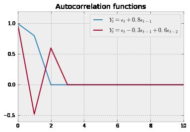
16 Autocorrelation Function

17 AR(1) Model Y t = φ 1 Y t 1 + Z t From the perspective of a linear dierence equation, Y t can be solved for as a function {Z t } via backwards subsitution: J 1 Y t = φ 1 ɛ t 1 + φ 2 Y t 2 + ɛ t (1) j=0 = ɛ t + φ 1 ɛ t 1 + φ 2 1ɛ t (2) = φ j ɛ 1 t j (3) j=0 How do we know whether this is covariance stationary?

18 Analysis of AR(1), continued We want to know if Y t converges to some random variable as we consider the innite past of innovations. The relevant concept (assuming that E[Y 2 t ] < ) is mean square convergence. We say that Y t converges in mean square to a random variable Y if E [ (Y t Y ) 2] 0 as n. It turns out that there is a connection to deterministic sums j=0 a j. We can prove mean square convergence by showing that the sequence generated by partial summations satises a Cauchy criteria, very similar to the way you would for a deterministic sequence.

19 Analysis of AR(1), continued What this boils down to: We need square summability: j=0 (φj 1 )2 <. We'll often work with the stronger condition absolute summability : j=0 φj 1 <. For the AR(1) model, this means we need φ 1 < 1, for covariance stationarity.

20 Relationship Between AR and MA Processes You may have noticed that we worked with the innite moving average representation of the AR(1) model to show convergence. We got there by doing some lag operator arithmatic: (1 φ 1 L)Y t = ɛ t We inverted the polynomial φ(z) = (1 φ 1 z) by (1 φ 1 z) 1 = 1 + φ 1 z + φ 2 1z Note that this is only valid when z < 1 = we can't always perform inversion! To think about covariance stationarity in the context of ARMA processes, we always try to use the MA( ) representation of a given series.

21 A General Theorem If {X t } is a covariance stationary process with autocovariance function γ X ( ) and if j=0 θ j <, than the innite sum Y t = θ(l)x t = θ j X t j j=0 converges in mean square. The process {Y t } is covariance stationary with autocovariance function γ(h) = θ j θ k γ x (h j + k) j=0 k=0 If the autocovariances of {X t } are absolutely summable, then so are the autocovrainces of {Y t }.

22 Back to AR(1) Y t = φ 1 Y t 1 + ɛ t, ɛ t WN(0, σ 2 ), φ 1 < 1 The variance can be found using the MA( ) representation Y t = φ j ɛ 1 t j = j=0 This means that [( ) ( )] E[Yt 2 ] = E φ j ɛ 1 t j φ j ɛ 1 t j = j=0 j=0 E [ ] φ 2j ɛ 2 t j = φ 2j σ 2 (4) j=0 σ2 γ(0) = V[Y t ] = 1 φ 2 1 j=0

23 Autocovariance of AR(1) To nd the autocovariance: Y t Y t 1 = φ 1 Y 2 t 1 + ɛ t Y t 1 = γ(1) = φ 1 γ(0) Y t Y t 2 = φ 1 Y t 1 Y t 2 + ɛ t Y t 2 Y t Y t 3 = φ 1 Y t 1 Y t 3 + ɛ t Y t 3 Let's look at autocorrelation ρ(τ) = γ(τ) γ(0) = γ(2) = φ 1 γ(1) = γ(3) = φ 1 γ(2)

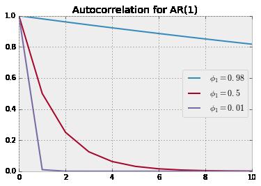
24 Autocorrelation for AR(1)

25 Simulated Paths

26 Analysis of AR(2) Model Which means Y t = φ 1 Y t 1 + φ 2 Y t 2 + ɛ t φ(l)y t = ɛ t, φ(z) = 1 φ 1 z φ 2 z 2 Under what conditions can we invert φ( )? Factoring the polynomial 1 φ 1 z φ 2 z 2 = (1 λ 1 z)(1 λ 2 z) Using the above theorem, if both λ 1 and λ 2 are less than one in length (they can be complex!) we can apply the earlier logic succesively to obtain conditions for covariance stationarity. Note: λ 1 λ 2 = φ 2 and λ 1 + λ 2 = φ 1

27 Companion Form [ Yt Y t 1 ] = [ φ1 φ ] [ Yt 1 Y t 2 ] + [ ɛt 0 ] (5) Y t = FY t 1 + ɛ t F has eigenvalues λ which solve λ 2 φ 1 λ φ 2 = 0

28 Finding the Autocovariance Function Multiplying and using the symmetry of the autocovariance function: Y t : γ(0) = φ 1 γ(1) + φ 2 γ(2) + σ 2 (6) Y t 1 : γ(1) = φ 1 γ(0) + φ 1 γ(1) (7) Y t 2 : γ(2) = φ 1 γ(1) + φ 1 γ(0) (8). (9) Y t h : γ(h) = φ 1 γ(h 1) + φ 1 γ(h 2) (10) We can solve for γ(0), γ(1), γ(2) using the rst three equations: (1 φ 2 )σ 2 γ(0) = (1 + φ 2 )[(1 φ 2 ) 2 φ 2] 1 We can solve for the rest using the recursions. Note pth order AR(1) have autocovariances / autocorrelations that follow the same pth order dierence equations.

29 Why are we so obsessed iwth autocovariance/correlation functions? For covariance stationary processes, we are really only concerned with the rst two moments. If, in addition, the white noise is actually IID normal, those two moments characterize everything! So if two processes have the same autocovariance (and mean... ), they're the same. We saw that with the AR(1) and MA( ) example. How do we distinguish between the dierent processes yielding an identical series?

30 Invertibility Recall φ(l)y t = θ(l)ɛ t We already discussed conditions under which we can invert φ(l) for the AR(1) model to represent Y t as an MA( ). What about other direction? An MA process is invertible if θ(l) 1 exists. so $MA(1) : θ 1 <1, MA(q):... $

31 MA(1) with θ 1 > 1 Consider Y t = ɛ t + 0.5ɛ t 1, ɛ t WN(0, σ 2 ) γ(0) = 1.25σ 2, γ(1) = 0.5σ 2. vs. Y t = ɛ t + 2 ɛ t 1, ɛ t WN(0, σ 2 ) γ(0) = 5 σ 2, γ(1) = 2 σ 2 For σ = 2 σ, these are the same! Prefer invertible process: 1. Mimics AR case. 2. Intuitive to think of errors as decaying. 3. Noninvertibility pops up in macro: news shocks!

32 Why ARMA, again? ARMA models seem cool, but they are inherently linear Many important phenomenom are nonlinear (hello great recession!) It turns out that any covariance stationary process has a linear ARMA representation! This is called the Wold Theorem; it's a big deal.

33 Wold Decomposition Theorem Any zero mean covariance stationary process {Y t } can be represented as Y t = ψ j ɛ t j + κ t j=0 where ψ 0 = 1 and j=0 ψ2 j <. The term ɛ t is white noise are represents the error made in forecasting Y t on the basis of a linear function of lagged Y (denoted by Ê[ ]): ɛ t = y t Ê[Y t y t 1, y t 2, ] The value of κ t is uncorrelated with ɛ t j for any value of j, and can be predicted arbitrary well from a linear function of past values of Y : κ t = Ê[κ t y t 1, y t 2, ]

34 Strict Stationarity A time series is strictly stationary if for all t 1,..., t k, k, h T if Y t1,..., Y tk Y t1 +h,..., Y tk +h What is the relationship between strict and covariance stationarity? {Y t } strictly stationary (with nite second moment) = covariance stationarity. The corollary need not be true! Important Exception if {Y t } is gaussian series covariance stationarity = strict stationarity.

35 Ergodicity In earlier econometrics classes, you (might have) examined large sample properties of estimators using LLN and CLT for sums of independent RVs. Times series are obviously not independent, so we need some other tools. Under what conditions do time averages converge to population averages. One helpful concept: A stationary process is said to be ergodic if, for any two bounded and measurable functions f : R k R and g : R l R, lim E [f (y t,..., y t+k )g(y t+n,..., g t+n+l ] n E [f (y t,..., y t+k )] E [g(y t+n,..., y t+n+l ] = 0 Ergodicity is a tedious concept. At an intuitive level, a process if ergodic if the dependence between an event today and event at some horizon in the future vanishes as the horizon increases.

36 The Ergodic Theorem If {y t } is strictly stationary and ergodic with E[y 1 ] <, then 1 T T y t E[y 1 ] t=1 CLT for strictly stationary and ergodic processes_ If {y t } is strictly stationary and ergodic with E[y 1 ] <, E[y 2 1 ] <, and σ 2 = var(t 1/2 y t ) σ 2 <, then 1 T σt T t=1 y t N(0, 1)

37 Facts About Ergodic Theorem 1. iid sequences are stationary and ergodic 2. If {Y t } is strictly stationary and ergodic, and f : R R is a measurable function: Z t = f ({Y t }) Then Z t is strictly stationary and ergodic. (Note this is for strictly stationary processes!)

38 Example Example: an MA( ) with iid Gaussian white noise. Y t = θ j ɛ t j, j=0 θ j <. j=0 This means that {Y t }, {Y 2 t }, and {Y t Y t h } are ergodic! 1 T Y t E[Y 0 ], t=0 1 T t=0 Y 2 t E[Y 2 0 ], 1 T Y t Y t h E[Y 0 Y h ], t=0

39 Martingale Dierence Sequences {Z t } is a Martingale Dierence Sequence (with respect to the information sets {F t }) if E[Z t F t 1 ] = 0 for all t LLN and CLT for MDS Let {Y t, F t } be a martingale dierence sequence such that E[ Y t 2r ] < < for some r > 1, and all t. Then ȲT = T 1 T t=1 Y t p 0. Moreover, if var( T ȲT ) = σ 2 T σ2 > 0, then T Ȳ T / σ T = N (0, 1).

40 References Brockwell, P. J. and Davis, R. A. (1987). Time series: Theory and methods. Springer Series in Statistics. Hamilton, J. (1994). Time Series Analysis. Princeton University Press, Princeton, New Jersey.