LECTURE 9: GENTLE INTRODUCTION TO

Size: px

Start display at page:

Download "LECTURE 9: GENTLE INTRODUCTION TO"

Oscar Joseph
5 years ago
Views:

1 LECTURE 9: GENTLE INTRODUCTION TO REGRESSION WITH TIME SERIES

2 From random variables to random processes (cont d) 2 in cross-sectional regression, we were making inferences about the whole population based on a small sample a crucial assumption: random sampling the bridge between population characteristics (distribution of wages in a country) and the probabilistic machinery of random variables (distribution of a wage of a randomly drawn person) unfortunately, with time series, random sampling makes no sense: year GDP inflation unemp , , what would the underlying population be?

3 From random variables to random processes (cont d) 3 random sampling makes the characteristics of different individuals independent it is difficult to imagine that GDP in 2004 is independent of that in 2005 therefore, we will have to switch to a more advanced theoretical vehicle: random processes those who had taken courses in random processes would tell you it was difficult we will omit many mathematical details, and focus on the intuition

4 New issues with time series 4 good news: everything we learnt with cross-sectional data will be used in time-series analysis, too bad news: many new pitfalls that can spoil the analysis 1. trends and seasonality: can result in spurious regression (see next slide) 2. lags in economic behaviour: government s expenditure cuts will slowly percolate through the economy lagged effect (the effect of today s cuts will spread over quarters or even years) 3. persistence in time series: governments expenditure itself cannot change too dramatically from one year to another most real-life time series persistent, but the degree differs strong persistence of time series can again produce spurious regression (stationarity, unit-root issues) weak persistence problematic only if applies to u (serial correlation, or autocorrelation of u)

5 Spurious regression problem 5 both y and x both exhibit a monotonous trend, we will find a relationship even though they have nothing in common Example: Norwegian salmon production vs GDP in the U.S. the data in salmon.gdt contain two annual time series ( ) annual salmon production in Norway GDP in the U.S. (bln. of 2005 dollars) do you think that there is a strong causal relationship? estimated equation in Gretl: ^gdp = 1.34e *salmon (713) ( ) T = 29, R-squared = (standard errors in parentheses) Quizz: is salmon significant at the 5 % level? And how about 1 %?

6 Let s look at the time series first: 6

7 Fitted values are calculated as: 13,

8 Accounting for trends in the regressions 8 Option 1 detrend all time series, i.e. create new variables where the linear trends have been subtracted two steps involved: (1) regress x t on t (time, values 1,2,,n) (2) save residuals (this is the detrended x t ) salmon series and its linear trend detrended salmon series

9 Accounting for trends in the regressions (cont d) 9 Option 2: add variable t (time) to the estimated equation Option 1: results ^gdp_detrended = 1.46e *salmon_detrended (52.7) ( ) T = 29, R-squared = (standard errors in parentheses) Option 2: results ^gdp = 5.14e *salmon + 295*time (304) ( ) (9.90) T = 29, R-squared = (standard errors in parentheses) salmon coefficient identical, std. errors nearly identical can use both R-squareds different, but most variation explained by time in Option 2 use detrended dependent variable for the R-squared!

10 10 Frisch-Waugh-Lovell theorem ===================================================================== Dependent variable: gdp gdp_detrended gdp (1) (2) (3) (4) year *** * ( ) ( ) salmon ** ** ( ) ( ) salmon_detrended ** ( ) ( ) Constant -578, *** -38, * (19, ) (19, ) Observations R =====================================================================

11 Using dummies to account for specific events 11 Example: fertility equation frequency: annual data, gfr = the number of births per 1000 women aged ww2 = 1 for years , = 0 otherwise expected fertility β 0 β 1 gfr ww u t 0 1 2t t WW2 period time

14 Using dummies to account for specific events (cont d) 14 Example: fertility equation 2 pill = 0 before 1963, = 1 afterwards expected fertility β 0 β 1 gfr pill u t 0 1 t t contraceptive pill introduced time

16 16 gfr β β ww2 β pill u t 0 1 t 2 t t

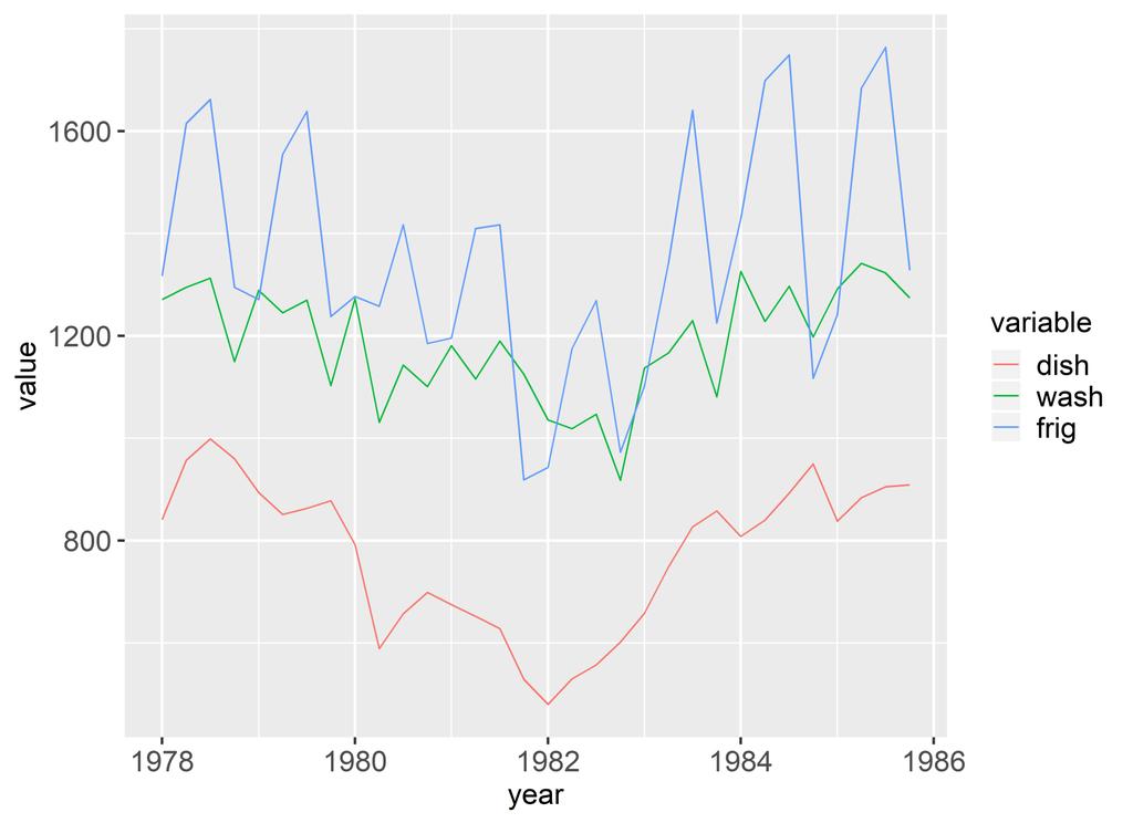
17 Seasonality 17 seasonal patterns are noticeable with quarterly, monthly, or daily data note that many time series in the online databases are seasonally adjusted, meaning that specialized algorithms have been used to even out the differences between seasons these series can be used without further ado when using a seasonally unadjusted series, we can still use a simple fix that accounts for the seasonal variation: periodic dummies, i.e. dummy variables that identify individual periods Example: durable goods open durgoods.gdt in Gretl change dataset structure to a quarterly time series (Data Dataset structure) add periodic dummies (Add Periodic dummies) this creates variables dq1,, dq4 (dq1 stands for dummy for quarter 1 )

18 18

19 values of the periodic dummies 19

20 Seasonality (cont d) 20 to describe the seasonal pattern in dishwasher sales, run the regression dish dq1 dq2 dq3 u t 0 1 t 2 t 3 t t the dishwasher time series and the fitted values are shown below, F-test for joint significance: p-value = 0.89 no statistical evidence of seasonality

21 Seasonality (cont d) 21 with refrigerator series, that s a different story: joint significance: p-value = , strong evidence of seasonality (i.e. we reject the null of no seasonal pattern)

22 Seasonality (cont d) 22 interpretation: just as with other category dummies we omitted dq4 quarter 4 is the base period e.g., the coefficient on dq1 tells us that in quarter 1, sales are higher by 62,125 than in quarter 4 (on average) Model 2: OLS, using observations 1978:1-1985:4 (T = 32) Dependent variable: frig coefficient std. error t-ratio p-value const e-018 *** dq dq *** dq e-05 *** Mean dependent var S.D. dependent var Sum squared resid S.E. of regression R-squared Adjusted R-squared F(3, 28) P-value(F)

23 Seasonality (cont d) 23 conclusion: with seasonally unadjusted data, it makes sense to add both a time trend and periodic dummies in addition to your independent variables of interest note that this can be done also in case the dependent variable is logged, only the interpretation changes: ^l_frig = *dq *dq *dq3 (0.0458)(0.0647) (0.0647) (0.0647) T = 32, R-squared = (standard errors in parentheses) results imply that in quarter 1, sales increase by 5.3 % compared with the baseline level of quarter 4

24 ^l_frig = *dq *dq *dq *time *sq_time (0.0590)(0.0470) (0.0471) (0.0473) ( ) ( ) T = 32, R-squared = Null hypothesis: the regression parameters are zero for the variables dq2, dq3, dq4 Test statistic: F(3, 26) = , p-value e-007

25 Finite distributed lag (FDL) model 25 Example: fertility equation 3 pe = real dollar value of personal tax exemption gfr pe pe pe pe u t 0 0 t 1 t1 2 t2 3 t3 t here, δ 0 is the impact propensity (= immediate effect) of a unit increase in pe the δ parameters capture the effect of a temporary increase in pe: assume that pe equals c except for period 0, where it increases to c + 1: pe t c time

27 pe t 1 c pe t 1 1 c pe t 2 pe t 3 c c 1 1 a temporary change in pe occurs in subsequent periods in lagged versions of pe gfr t d δ 0 δ 1 δ 2 δ 3 the effect of a temporary change in pe, or the lag distribution time 27

29 Finite distributed lag (FDL) model (cont d) 29 long-run propensity (LRP): the effect of a permanent unit increase in pe LRP pe t 1 c gfr t d δ 0 δ 1 δ 2 δ 3 the effect of a permanent change in pe, or long-run propensity time

31 gfr β β ww2 β pill β t δ pe δ pe δ pe δ pe u t 0 1 t 2 t 3 0 t 1 t 1 2 t 2 3 t 3 t

32 Finite distributed lag (FDL) model (cont d) 32 Estimating LRP a natural estimator of LRP is LRP ˆ ˆ ˆ ˆ so we just add up the coefficients on pe and its lags more work is required in case we need std. errors or 95% CI for LRP we ll use a simple trick: the equation can be rewritten as follows gfr pe pe pe pe u t 0 0 t 1 t1 2 t2 3 t3 t LRP pe ( pe pe ) ( pe pe ) ( pe pe ) u 0 t 1 t1 t 2 t2 t 3 t3 t t A B C this gives us the following procedure: 1. Create variables A, B, and C. in Gretl: Add Define new variable A = pe( 1) pe etc. 2. Regress gfr on pe, A, B and C; now, LRP is the coefficient on pe, and we can read off its std. error and calculate the 95% CI if needed.

33 LECTURE 9: GENTLE INTRODUCTION TO REGRESSION WITH TIME SERIES

Outline. 11. Time Series Analysis. Basic Regression. Differences between Time Series and Cross Section

Outline. 11. Time Series Analysis. Basic Regression. Differences between Time Series and Cross Section Outline I. The Nature of Time Series Data 11. Time Series Analysis II. Examples of Time Series Models IV. Functional Form, Dummy Variables, and Index Basic Regression Numbers Read Wooldridge (2013), Chapter