20th Summer Institute in Statistical Genetics

Transcription

1 th Summer Institute in Statistical Genetics

2 (This page left intentionally blank.)

3 SYLLABUS PRINCIPLES OF QUANTITATIVE GENETICS INSTRUCTORS: William Muir, Department of Animal Sciences, Purdue University Bruce Walsh, Department of Ecology & Evolutionary Biology, University of Arizona LECTURE SCHEDULE Monday, 3 July 8:3 : am. Population Genetics Framework (Muir) : :3 am Break :3 :. Fisher s Variance Decomposition (Muir) Background reading: LW Chapter 4 : :3 pm Lunch :3 3: pm 3. Resemblance Between Relatives, Heritability (Muir) Background reading: LW Chapter 7 3: 3:3 pm Break 3:3 5: pm 4. Artificial Selection (Walsh) Background reading: WL Chapter 3 Additional reading: WL Chapters 4-6 Tuesday 4 July 8:3 : am 5. Inbreeding and Crossbreeding (Walsh) Background reading: LW Chapter : :3 am Break :3 : 6. Correlated Characters (Walsh) Additional reading: WL Chapters : :3 pm Lunch :3 3: pm 7. Mixed Models, BLUP Breeding Values, REML (Muir) Background reading: LW Chapter 6 Additional reading: WL Chapters 9, 3: 3:3 pm Break 3:3 5: pm 8. QTL/Association Mapping (Walsh) Background reading: LW Chapters 5, 6 Evening Open session (review, R, etc)

4 Wednesday, 5 July 8:3 : am 9. Tests for Molecular Signature of Selection (Walsh) Background reading: Additional reading: : :3 am Break :3 :. More on Mixed Models, BLUP Breeding Values (Muir) Additional reading: WL Chapters 8 - Website for draft chapters from Volume : Walsh & Lynch: Evolution and Selection on Quantitative traits ADDITIONAL BOOKS ON QUANTITATIVE GENETICS General Falconer, D. S. and T. F. C. Mackay. Introduction to Quantitative Genetics, 4 th Edition Lynch, M. and B. Walsh Genetics and Analysis of Quantitative Traits. Sinauer. Roff, D. A Evolutionary Quantitative Genetics. Chapman and Hall. Mather, K., and J. L. Jinks. 98. Biometrical Genetics. (3 rd Ed.) Chapman & Hall. Animal Breeding Cameron, N. D Selection Indices and Prediction of Genetic Merit in Animal Breeding. CAB International. Mrode, R. A Linear Models for the Prediction of Animal Breeding Values. CAB International. Simm, G Genetic Improvement of Cattle and Sheep. Farming Press. Turner, H. N., and S. S. Y. Young Quantitative Genetics in Sheep Breeding. Cornell University Press. Weller, J. I.. Quantitative Trait Loci Analysis in Animals. CABI Publishing. Plant Breeding Acquaah, G. 7. Principles of Plant Genetics and Breeding. Blackwell. Bernardo, R.. Breeding for Quantitative Traits in Plants. Stemma Press. Hallauer, A. R., and J. B. Miranda Quantitative Genetics in Maize Breeding. Iowa State Press. Mayo, O The Theory of Plant Breeding. Oxford. Sleper, D. A., and J. M. Poehlman. 6. Breeding Field Crops. 5 th Edition. Blackwell

5 Wricke, G., and W. E. Weber Quantitative Genetics and Selection in Plant Breeding. De Gruyter. Humans Khoury, M. J., T. H. Beaty, and B. H. Cohen Fundamentals of Genetic Epidemiology. Oxford. Plomin, R., J. C. DeFries, G. E. McLearn, and P. McGuffin.. Behavioral Genetics (4 th Ed) Worth Publishers. Sham, P Statistics in Human Genetics. Arnold. Thomas, D. C. 4. Statistical Methods in Genetic Epidemiology. Oxford. Weiss, K. M Genetic Variation and Human Disease. Cambridge. Ziegler, A., and I. R. Konig. 6. A Statistical Approach to Genetic Epidemiology. Wiley. Statistical and Technical Issues Bulmer, M. 98. The Mathematical Theory of Quantitative Genetics. Clarendon Press. Kempthorne, O An Introduction to Genetic Statistics. Iowa State University Press. Saxton, A. M. (Ed). 4. Genetic Analysis of Complex Traits Using SAS. SAS Press. Sorensen, D., and D. Gianola.. Likelihood, Bayesian, and MCMC Methods in Quantitative Genetics. Springer.

6 Muir and Walsh Lecture Introduction to Quantitative Genetics Population Genetics Foundation Quantitative Genetics Quantitative Traits Continuous variation Varies by amount rather than kind Height, weight, IQ What is the Basis for Quantitative Variation?

7 Mendelian bases for Quantitative Genetics Early experiments by Nilsson-Ehle (98) Wheat color.6.5 Parents. F Dark red med DR medium red pale red white Dark red med DR medium red pale red white F Blending? What Mode of Inheritance Would Explain This? Dark red med DR medium red pale red white Would Blending Explain this? 4

8 Hypothesis: loci acting independently and cumulatively on one trait? Dark Red AABB (4) X White aabb () Medium Red AaBb () X Medium Red AaBb () Dark Red AABB (4) Medium Dark Red AABb (3) AaBB (3) Medium Red AaBb () AAbb () aabb () Pale Red Aabb () aabb () White aabb () /6 4/6 6/6 4/6 /6 Gene Effects Usual Mendelian Concept Gene Trait Gene Trait Simple Traits Gene Trait Trait Pleiotropy Genetic Correlation Between Traits Gene Gene Trait Polygenic Trait

9 What happens to the distribution as the number of loci increases? A continuous distribution emerges Stability of Distribution From Previous Example with Wheat F Dark red med DR medium red pale red.65 white What is the expected Distribution of the F3? F4?. Will it stay the same?. Will we see a reduction in variability? 3. Will we see and increase in variability? Need to know concepts of probability

10 Important Concepts of Probability Compound Events Two Events are Independent if Knowledge of one event tells us nothing about the probability of occurrence of the other event In General Pr(A and B)=Pr(A B)xPr(B) With Independence Pr(A B)=Pr(A) Pr(A) thus Pr(A and B)=Pr(A)xPr(B) What is the Consequence of Random Mating on Genotypic Frequencies Assume a Perfect World No Forces Changing Allele frequency No: mutation, migration, selection, genetic drift Equal Allele Frequencies in the Sexes Autosomal Inheritance Random Mating

11 GENERATION Allow The Genotypic Frequencies To Be Any Arbitrary Values genotypic frequency P( AA ) = X P( Aa ) = Y P( aa ) = Z such hthat tx+y+z + = Allele Frequencies P( A ) = P(AA) + P(Aa) P( A ) = X + Y = p P( a ) = P(aa) + P(Aa) P( a ) = Z + Y = q p + q =

12 Frequency of Mating male genotype female genotype AA Aa aa frequency ( X ) ( Y ) ( Z ) AA ( X ) X XY XZ Aa ( Y ) XY Y YZ aa (Z) XZ YZ Z Random Mating=independence Expected genotypic frequencies that result from matings (Gen ). Expected Frequency of Offspring Possible Frequency of AA Aa aa Matings Mating AA x AA X AA x Aa XY / / AA x aa XZ Aa x Aa Y /4 / /4 Aa x aa aa x aa YZ Z / / Conditional Probabilities given genotypes of parents

13 GENERATION P( AA offsping ) =( X = X = ) + ( + XY + ( X + Y ) XY ) + 4 Y 4 ( Y ) = Because [ P( A ) ] parents P( A ) = X + P( AA offspring Y = p Therefore for generation ) = p P(Aa offsping )= ( XY)+(XZ)+ =XY+XZ+ Y = +YZ ( X+ Y )( Z+ Y ) =pq (Y )+ (YZ) P( aa offsping ) = 4 = = ( Y 4 Y ) + ( YZ ) +( Z + YZ + Z ( Z + Y ) = q )

14 Generation Frequency of Matings male genotype female genotype AA Aa aa frequency ( p ) ( pq ) ( q ) AA ( p ) p 4 p 3 q p q Aa ( pq ) p 3 q 4p q pq 3 aa ( q ) p q pq 3 q 4 Expected genotypic frequencies that result from matings (Gen ). Expected Frequency of Offspring Possible Frequency of AA Aa aa Matings Mating AA x AA p 4 AA x Aa 4p 3 q / / AA x aa p q Aa x Aa 4p q /4 / /4 Aa x aa aa x aa 4pq 3 q 4 / /

15 Overall Genotypic Frequencies 4 3 P( AA p ) + p q) + offsping) =( ( 4 ( 4p q = p + p q + p q = p = p = p ( p +pq+ q ) ( p + q ) P( Aa ) = offsping = p () pq ) P( aa ) = offsping q Summary of genotypic frequencies by Generation genotype gen gen gen P( AA ) X p p P( Aa ) Y pq pq P( aa ) Z q q

16 Hardy-Weinberg Equilibrium or the Squared Law If a population starts with any arbitrary distribution of genotypes, provided they are equally frequent in the two sexes, the proportions of genotypes (AA, Aa, aa), with initial allele frequencies p and q, will be in the proportion ( ) p + q = p + ( pq ) + q A a AA Aa aa after one generation of random mating and will remain in that distribution until acted upon by other forces Stability of Distribution From Previous Example with Wheat F Dark red med DR medium red pale red.65 white What is the expected Distribution of the F3? F4?. Will stay the same (assumptions?). Will see a reduction in variability (how, when)? 3. Will see and increase in variability(how, when)?

17 Example Population Cage Introduce 4 males ( round eye and 3 star eye), and 4 females ( round and 3 star eye). Assume co-dominance of eye shape where heterozygotes are square eyed. AA Aa aa What are the initial allele frequencies for eye shape? What are the expected frequencies of eye shapes in G and G 3 Example Population Cage Introduce 4 males ( round eye and 3 star eye), and 4 females ( round and 3 star eye). Assume co-dominance of eye shape where heterozygotes are square eyed. What are the initial allele frequencies for eye shape? What are the expected frequencies of eye shapes in G and G AA Aa aa Note same frequency in both sexes P A=3/4+/()=3/4 G=(3/4A+/4a) = 9/6AA 6/6Aa /6aa P A=9/6+/(6/6)=/6=3/4 G= (3/4A+/4a) = 9/6AA 6/6Aa /6aa 4

18 What if Organisms Do not Mate But Release Gametes or Pollen to Search Out Each Other? Do the Same Properties Hold? Fertilization Given a female gamete carrying the a allele, what is the probability it will be fertilized by a gamete (pollen) carrying the A allele If Independence P(A a)=p(a) If not Independence P(A a )= to Incompatibility

19 What is the Consequence of Random Union of Gametes Assume a Perfect World No Forces Changing Allele Frequency Equal Allele Frequencies in the Sexes Autosomal Inheritance GENERATION lets allow the genotypic frequencies to be any arbitrary value and the allelee frequencies to be the appropriate function of those values. genotypic frequency P( AA ) = X P( Aa ) = Y P( aa ) = Z such that X + Y + Z =

20 Allele Frequency P( A ) = X + = p P( a ) = Z + = q Y Y p + q = With Independence male gamete/frequency A a ( p ) ( q ) female gamete/ A AA Aa frequency ( p ) ( p ) ( pq ) a Aa aa ( q ) ( pq ) ( q ) Random Union of Gametes Produces the Same Outcome as Random Mating

21 What Happens If The Allele Frequencies Are Not Equal Between The Sexes? Generation Gametic Frequencies A Male Gamete Frequency a p m q m Female Gamete frequency A a p f q f p p p q m f f m AA Aa Genotypic Frequencies Generation p q q q m f m f aa Aa Each genotype is equally divided between sexes Gametic Frequencies Produced by Adults in First Generation Frequency of Homozygous Class + ½ frequency of heterozygous class ( p q p q ) p m = p f = pm p f + m f + Because an equal number of both sexes are produced from each mating f m Note, because gametic frequencies are now equal in sexes p m = p f = p 3

22 Generation Gametic Frequencies Female Gamete frequency A a Generation A Male Gamete Frequency a p p p p = ( p ) p q AA Aa q Genotypic Frequencies in Generation q ( ) p Aa Population in HW by nd generation q q = The one generation delay before reaching HW can be very informative aa q q Introduce 4 males ( round eye and 3 star eye), and 4 females (3 round and star eye). Assume co-dominance of eye shape where heterozygotes are square eyed. Example AA Aa aa What are the initial allele frequencies for eye shape? What are the expected frequencies of eye shapes in G and G 34

23 Example Cross Between Populations G Population Population Males Females ¾ AA ¼ aa ¼ AA ¾ aa What are the expected allele frequencies, and genotypic frequencies in each generation? G G Random Mate Generation Population Population Males Females ¾ AA ¼ aa ¼ AA ¾ aa ¼ A ¾ a ¾A ¼ a 3/6 AA 9/6 Aa /6 Aa 3/6 aa p =3/6 + ½(9/6 + /6)=8/6= ½ G Genotypic Freq G Allele Freq

24 Generation GMales 3/6 AA /6 Aa 3/6 aa GFemales 3/6 AA /6 Aa 3/6 aa ½ A ½ a ½A ¼AA ¼Aa ½ a ¼ Aa ¼ aa p = ¼ + ½( ¼ + ¼ )= ½ G Genotypic Freq G Allele Freq G Population Males ¾AA ¼aa Summary Population Females ¼AA ¾aa G 3/6 AA /6 Aa 3/6aa p = ½ Genotypic Frequencies Different G 4/6 AA 8/6 Aa 4/6aa p = ½ Allele Frequencies Same G3?

25 Sample Genotype Distribution Important Example ( p q ) = p + ( pq ) + q = A + a AA Aa aa HWE Expected Distribution 3/6 AA Too Many 4/6 AA /6 Aa heterozygotes 8/6 Aa 3/6 aa in Sample 4/6aa This is also an example of a genomic pattern of recent crossing between populations with immigrants of one sex Question : will this pattern affect all loci? (yes and no, why?) This is said to be a pattern of demography, why? Question :If the immigration only occurs once, will the pattern of demography disappear with time? If so, how many generations will it take? Question 3: If an equal number of males and females were among the migrants, and mating was totally at random, regardless of origin, will there be a pattern of excess of heterozygotes? Consider just No Indian Heritage (), 5% (4) and pure American Indian (8) Would you expect each of these sub-populations to conform to H-W distributions? Why?

26 Observed Expectations Expected heritage Gm/Gm Gm/non non/non Total Pgm Pnon / / heritage Gm/Gm Gm/non non/non / / Deviation from Expectation heritage Gm/Gm Gm/non non/non heterozygotes deviation from expecation / slightly deficient 4/ Great Excess slightly deficient In this example we were able to determine the heritages and population structure by questioning In what ways could this example be applied to situations where we can t ask? What could cause a deficiency in heterozygotes as compared to expectation? Sampling Across Sub-populations Unknowingly Sample Population Males and Females AA Population Males and Females aa ( ) pa + qa = paa + ( pq ) Aa + qaa 5% AA HWE Sample 5% AA Genotype % Aa 5% Aa Expected Distribution 5% aa 5% aa Distribution Too few heterozygotes in Sample = Admixture p.5 + ( ).5 A = = 4

27 Admixture Pima Indians Combined pure American Indian (8) and Non () Gm/Gm Gm/non non/non Total Pgm Pnon / total Expected Gm/Gm Gm/non non/non / total Deviation from Expectation Gm/Gm Gm/non non/non heterozygotes deviation from expecation / total Too Few Sampling Across Populations = Admixture Too few heterozygotes in sample as compared to HWE = Signal of Admixture Admixture results from sampling across populations Question : will this pattern affect all loci? (yes and no, why?) This is also said to be a pattern of demography, why Question :If the races remain distinct (pure) will the signature of demography disappear with time? If so, how many generations? 44

28 HWE and the so what question HWE establishes the null hypothesis for expectations Deviations from expectations are where all the interesting problems and Issue occur Lecture Problems. Two separate populations of equal size are in equilibrium for the same pair of alleles because of random mating within each. In population I, p A =.6, while in population II, p A =., with q = - p in each population. (a) If a random sample of females from one population is crossed to a random sample of males from the other population, what would be the expected genotypic frequencies among the progeny? If these progeny are then allowed to mate at random, what would be the expected allele and genotypic frequencies in the next-generation? What happens to heterozygote frequencies between the F and F generations? (b) If equal numbers of both sexes from each population are combined and allowed to mate at random, what would be the expected allele l and genotypic frequencies in the next-generation? (c) Compare results in part a and b, what conclusions can you draw from this.

29 Muir Lecture Quantitative Traits Fisher Decomposition Covariance Between Relatives Phenotype (Y) Quantitative Traits Continuous (Weight) semi-continuous scale (Egg number) Some Discrete Traits (Disease Resistance) Underlying distribution assumed continuous Polygenic (G) Environmentally Influenced (E) Y = G + E i i i

30 Variances Genetic sources of variation Partially underlie trait variation Inferred from statistical sources of variation Statistical Sources of variation Variation among and within identifiable groups (families) 3 Partitioning sources of variation general case Classic ANOVA model for two Treatments, A and B, each with levels Treatment A Treatment B B B A A interaction effect Y ij = μ + A + B + AB + ε i j ij (ij) Main Effects Random error 4

31 Applied to genetics Treatment A results from alleles from the Father Treatment B results from alleles from the Mother Male parent Allele Model m α m α Female Parent Allele Yij f α f α Y Y Y Y Intra-locus interaction (dominance) = μ + α + α + δ + ε f i m j ij (ij) If we assume allele effects from mother are the same as from the father (no imprinting) Yij = μ + α + α + δ + ε i j ij (ij) 5 Male parent Allele p p Allelic effects and intra locus interactions α α Female Parent Allele p α p α Y Y Y Y α = p Y i i μ i= α = p Y i i i= Yij μ = μ + α + α + δ i Fit model E( ( ε ) = α = p Y j j μ j= α = p Y j j μ μ j= = i j p p Y Questions: δij = Yij μ αi α j What is the expected frequency of Y? What assumption is being made to find expected frequency? Will these expectations be valid if there is admixture or recent crossing? i j j ij 6 ij

32 In General So A = Genetic Variances Mean Variance Additive Variance σ = i p α i = Y i i = fiy ( f ) iy = σ Y = fi Yi i = σ Dominance Variance = σ σ D i j p p δ i j ij D A = = i j f α i i i j p p δ ( f iα i ) ij ( fijδij ) 7 Additive Variation Additive variation=variation due to effects of single alleles Alleles are passed on in haploid state, thus only the effect of a single allele is inherited from one parent Breeding for superior traits or natural selection is based on what can be passed on in the haploid state, i.e. single allele effects Additive variation=useable variation 8

33 Non-additive Variation Dominance Variation Due to intra-locus interaction Requires both alleles at a locus to express Cannot be passed on by one parent Not useable for selective breeding Epistatic Variation Due to inter-locus interactions Requires interaction of,3, or 4 alleles at two loci Not useable for selective breeding Yes alleles at different loci can be inherited in the haploid state but recombination in following generation(s) will break up 9 Male parent Allele α α Example Genetic Effects, known genotypes In a randomly mating population Female Parent Allele 3 p = p 4 = 4 α α 4 α α Yij Fit = μ + α + α + δ i E ( ε ) = ( ) + ( ) = = 4 4 ( ) + ( 4).75 =. 5 3 = 4 4 j ij α = = α μ = 9 ( ) + 3 ( ) + 3 ( ) + ( 4) = Note: piα i = p α + pα = ( 75) + (.5) = i 4 By construct!. 4

34 Genetic Variances (known genotypes and frequencies) p α = [ (.75) (.5) ] 3 + = σ A = p i i 4 4 i δij = Yij μ αi α j δ =.75 (.75) =.5 δ = δ =.75 (.75) (.5) δ σ D = = 4.75 (.5) 5) =.55 = i j p p δ i j ij = (.5) + ( )(.75) + ( )(.5) = Breeding Values Breeding value is the genetic worth of an animal (what we expect the animal to pass on to its progeny) EBV ( Y ij ) = α i + α j EBV ( Y ) = α + α = (.75) =.5 EBV ( Y ) = (.75) + (.5) =.5 EBV ( Y ) = (.5) = 4.5 What is the expected performance of the progeny of two parents whose breeding values are EBVa and EBVb? Yˆ = μ + ( EBVa + EBVb)

35 Covariance Between Relatives Needed to associate genetic source of variance with statistical source of variation Separate genetic sources of variation into additive vs. non-additive Separate genetic sources of variation from environmental The entire underpinning to quantitative genetics 3 Genetic Covariance Relatives are more likely to share alleles than non-relatives Sharing Alleles = Identical by Descent (IBD) Identically same allele can be traced to an ancestor Statistical Concept Not to be confused with Alike in State t (AIS) If two alleles are AIS they maybe IBD If two alleles are not AIS then they cannot be IBD 4

36 Single Parent-offspring Covariance P P A A A A δ α α + + = G P A A A 3 A 4 % of the time parent and offspring will share one and only one allele) x x O G δ α α + + = ½ A A x ½ A A x x x O G δ α α + + = 5 ), ( ), ( ), ( x x x x O P Cov Cov G G Cov δ α α δ α α δ α α δ α α = Single Parent-offspring Covariance -IBD = ), ( ), ( ), ( ), ( ), ( ), ( ), ( ), ( ), ( ), ( x x x x x x O P Cov Cov Cov Cov Cov Cov Cov Cov Cov G G Cov δ δ α δ α δ δ α α α α α δ α α α α α -IBD ), ( ), ( ), ( ), ( ), ( ), ( ), ( ), ( ), ( x x x x x x Cov Cov Cov Cov Cov Cov Cov Cov Cov δ δ α δ α δ δ α α α α α δ α α α α α 6

37 Cov( α, α ) i In General: Covariance between effects j = σ A Additivity is a function of single alleles Cov( α, δ ) = i ij Cov( δ ij, δ km) σ = D if i j, i.e. not IBD if i = j, i.e. IBD By construct (residuals are found as deviations from main effects) if i j km, i.e. both not IBD if i j= km, i.e. both IBD Dominance is a function of two alleles at the same locus, it is estimated here as the failure of both alleles at that locus to be additive. σ = α σ A p i i i D = pi p jδij i j Question: What is epistasis a function of? 7 Single Parent-offspring Covariance -IBD Cov( GP, GO ) = Cov( α + α + δ, α + α x + δ + Cov α + α + δ, α + α + δ ) Cov ( x x -IBD ( G P, G O ) = ( ) σ A ( σ ) + A + x ) Cov ( G, G ) = σ P O A 8

38 Summary Single Parent-Offspring Number of IBD IBD alleles IBD alleles IBD alleles Probability of Sharing Contribution to variances σ A σ + A σ D Cov( G P, GO ) Total covariance=sum Probability x contribution= σ = () σ + ()( σ + σ ) P. O A A D σ = σ P. O A 9 Collateral: Half sibs A 3 A 4 A A A5 A 6 O O A 3 A 4 A A ¼ ¼ ¼ ¼ A 5 A 6 A A ¼ ¼ ¼ ¼ Cov ( G, G O ) O

39 Collateral: Number of IBD Alleles Sib O possible genotypes A A 3 A A 4 A A 3 A A 4 /4 /4 /4 /4 Sib O possible genotypes A A 5 ¼ A A 6 ¼ A A 5 ¼ A A 6 ¼ Collateral: Half sibs Number of IBD IBD alleles IBD alleles IBD alleles Probability of Sharing 8/6 8/6 Contribution to variances σ A A σ D σ + Cov( G O, G ) O Total covariance=sum Probability x contribution= σ = = HS ( 8 6) σ A 4 σ A

40 Collateral: Full sibs A 3 A 4 A A O O A 3 A 4 A A ¼ ¼ ¼ ¼ A 3 A 4 A A ¼ ¼ ¼ ¼ Cov( G O, G O ) = σ FS 3 Collateral: Number of IBD Alleles Sib O possible genotypes A A 3 A A 4 A A 3 A A 4 /4 /4 /4 /4 Sib O possible genotypes A A 3 ¼ A A 4 ¼ A A 3 ¼ A A 4 ¼ 4

41 Collateral: Full sibs Number of IBD IBD alleles IBD alleles IBD alleles Probability of Sharing 4/6 8/6 4/6 Contribution to variances σ A A σ D σ + Cov( G O, G ) O Total covariance=sum Probability x contribution= FS 8 4 ( )( σ ) + ( )( σ + σ ) = σ σ σ = + 6 A 6 A D A 4 D Question: genetically, are you more similar to your mother or full sister? 5 Covariance Between Relatives in General Cov G x, G ) ( y Number of IBD Probability of Sharing Contribution to variances IBD alleles IBD alleles Pr() xy Pr() xy σ A A σ D σ + Let a ) xy = Pr() + xy Pr( xy u xy = Pr() xy Additive relationship Cov( G x, G Total covariance=sum contributions= y ) Cov ( Gx, Gy ) = axyσ A + uxyσ D With higher order effects (epistasis) = axyσ A + uxyσ D + axyσ AA + axyuxyσ AD + uxyσ DD Dominance Relationship

42 Problem Falconer (98) reported a partially dominant gene in the mouse called pg pygmy. At six weeks of age, it produces the following average weight phenotypes in grams: + / + : 4, + / pg :, pg / pg : 6 (a) What is the additive effect of each + substitution? What would be the expected mean, additive and dominance variance in a population with p + =.8, q pg =. under random mating?? (b) If p + = q pg, What average effect of an allele substitution? what would be the mean additive and dominance variance? 7 Problem a Answer + pg.8. Alpha(i) pg Alpha(i) var sig(a) Dominance sig(d) 8

43 Problem b Answer Lesson: Additive genetics variance is dependent on allele frequencies + pg.5.5 alpha pqa pg alpha - 4 pa 4 8 sig(a).5.5 Dominance.5 - dev.5 - sig(d) 9 Problem Consider the following phenotypes: A A = 8 A A = A A = (a) If p =., q =.8, What is the effect of an allele substitution? what would be the mean additive and dominance variance? (b) If p =.8, q =. What is the effect of an allele substitution? What would be the expected mean, additive and dominance variance? (c) Considering these results, what are the limitations of working backward and drawing conclusions about gene action from calculations of variance components? 3

44 Problem a Answer + pg..8 alpha Var pg alpha var sig(a)..8 Domina nce dev sig(d) 3 Problem b answer Lesson: All of the genetic variability here is due to non-additive effects. With natural selection on viability and overdominance this is the equilibrium allele frequency. + pg.8. Alpha(i) pg Alpha (i) var sig(a).8. Dominance dev sig(d) 3

45 Muir Lecture 3 Computation of Additive Relationships Genetic covariance between relatives Cov a xy ( Gx, Gy ) = axyσ A + uxyσ D Heritability h and H Covariance Between Relatives x and y Cov = σ + σ ( Gx, Gy ) axy A uxy D Relationship due to joint IBD at a locus Relationship due to additive effects Depends on pedigree (IBD) Additive genetic variance Depends on trait allele frequencies gene Action Non-additive effects cannot be passed from parent to offspring as a unit (meiosis splits pairs) except as clones Important for heterosis and crossbreeding programs

46 Recursive Method to Compute Additive Relationships a xy Setup pedigree table from oldest to youngest (parents must occur before offspring, genes flow in one direction) For parents unknown, assume they are unrelated to each other and non-inbred Compute following from oldest to youngest a ij = a ji a = + ii = a ( a + a ) i s i, d i, js i, jd 3 Example In the following pedigree find the additive relationship between all individuals A B C D 4

47 A B???? A B A B C D A B C D A ½ (a AA +a AB ) ½(a AA +a AB ) ½ (+)= ½ ½ (+)= ½ B ½(a BA +a BB ) ½ (+)= ½ ½ (a BA +a BB ) ½ (+)= ½ C D + ½ a AB += ½ (a CA +a CB ) ½ (½ +½)= ½ + ½ a AB += 5 A C B D?,??,? A,B A,B A B C D A ½ ½ B ½ ½ C ½ ½ ½ D ½ ½ ½ 6

48 Example A B C Find all relationships note that D is the result of mating relatives D 7 A C B?,??,? A,B A,C A B C D D A ½(a (aaa +a AB ) ½(a AA +a AC ) B sym ½ (a BB +a BA ) ½ (a BA +a BC ) C sym + ½ a AB ½ (a CC +a AC ) D sym + ½ a AC 8

49 A D C B?,??,? A,B A,C A B C D A ½ (+)= ½ ½ (+ ½)=3/4 B ½ (+)= ½ ½ (+ ½)=/4 C sym [+ ½ ()] ½ (+ ½)=3/4 D sym [ + ½(½)] =5/4 9 Example Given the following pedigree, find all additive relationship and inbreeding coefficients. Assume animals not given are unrelated and not inbred. Pedigree From Wright (9) given in Lynch and Walsh p 39. A B C D E F G H I J K

50 A Matrix by Excel.,. A,..,. A,. A,. B,C C,D E,. F,G C,H I,J A B C D E F G H I J K A B C D E F G H I J K amatrix LECTURE EXAMPLE by Excel.xlsx. a xy is a covariance between individuals due to shared IBD alleles, not a probability or a correlation (<a xy <).. a xy = x coefficient of relationship (Malecot, 948) Coefficient of Relationship (Malecot, 948) p(randomly chosen allele at a locus in individual id x is IBD with a randomly chosen allele at that locus in individual y)

51 Probability IBD non-related individuals coefficient of relationship =p(randomly chosen allele at a locus in individual x is IBD with a randomly chosen allele at that locus in individual y) X A A A 3 A 4 Y Random Allele Random Allele ¼ ½ A ¼ ¼ ½ A 3 ½ A P(IBD between unrelated individuals)= P(IBD)= /4P(A =A 3 )+ /4P(A =A 4 )+ /4P(A =A 3 )+ /4P(A =A 4 )= a xy =P(IBD)= this is why off diagonal element are for non-related individuals ¼ ½ A 4 3 What is the coefficient of relationship of an individual with itself? This is the same as asking what is the coefficient of relationship between the individual and its clone First consider a non-inbred clone From this find the additive relationship (a xy ) between non-inbred clones 4

52 Probability IBD between non-inbred Clones Non inbred means that the P(IBD) within and individual is or P(A =A )= X Clone X A A A A Random Allele Random Allele ¼ ½ A ½ A Not IBD ½ A ½ A ¼ P(IBD between Non-Inbred Clones)=/ a xy =P(IBD)= This is why the diagonal elements in A are for non-inbred individuals 5 Next: Consider the other extreme: What is the coefficient of relationship between completely inbred clones? Convert this probability to the additive relationship (a xy ) between perfectly inbred clones a xy =P(IBD) 6

53 Completely inbred means both two alleles at a locus are IBD X Clone X A A A A Random Allele Random Allele A A IBD % P(IBD Perfectly Inbred Clones)= a xy =P(IBD)= which is the maximum value for a diagonal element in the A matrix Inbreeding is why some of the diagonal element are > and is a method to estimate the inbreeding coefficient F x =a xx -. In this example F x =-= 7 Additive Relationship Matrix (A).,. A,..,. A,. A,. B,C C,D E,. F,G C,H I,J A B C D E F G H I J K A B C D E F G H I J K What is the inbreeding coefficient for individual K?. F k =.4-=.4 3. What is the additive relationship between individuals J and K 4. a jk = What is the additive genetic covariance between individuals J and K for trait T? for trait T? Cov( G, G ) = a σ Cov T T x x ( G, G ) = a σ x y y y xy Cov ( G, G ) = a σ xy xy A AT AT =.64σ =.64σ AT AT 8

54 Covariance Between Relatives Common Environmental Causes E c Common Farm Common Maternal Common Cage or Pen 9 Environmental Effects Common Environmental Effects Ec Can contribute to resemblance of relatives Can be corrected for using mixed models allowing for correlated residuals

55 Summary Resemblance Among Relatives for a Given Trait Relative Pair Any Set of Relatives Cov Cov ( Gx, Gy ) = axyσ A + σ Ec ( xy) σ +σ Parent-Offspring A E ( P. O) c Half-Sib 4 σ +σ A E ( HS ) c σ +σ Full-Sib A E ( FS ) c Heritability Broad Sense: Proportion of the phenotypic variation due to genetic causes H σ = σ G Y Narrow Sense: Proportion of the phenotypic variation due to additive genetic effects h σ = σ A Y Useful to determine to what extent genetics vs environment impact a trait Useful to determine to what extent directional selection can improve a trait

56 Examples of Heritabilities Organism Trait h Humans Height Serum IG.45 Pigs Back-fat thickness.7 Daily weight-gain.3 Litter size.5 Fruit flies Abdominal bristles.5 Body size.4 Ovary size.3 Egg production. 3 Estimation of Narrow Sense Heritability h σ σ = = σ σ + A Y G A σ ε Three Approaches Regression Analysis of Variance Maximum Likelihood (ML), REML, Gibbs Estimation of Variance Components All based on resemblance between relatives 4

57 Regression X Ancestor-Descendent Pairs Cov ( Gx, Gy ) = axyσ A Y Parent-offspring Grand-parent-grand son Great Uncle-Nephew Etc 5 Regression Francis Galton a half-cousin to C. Darwin established the principle of what he termed "regression to mediocrity. studied the inheritance of height in humans noticed that extremely tall fathers tended to have sons shorter than themselves, and extremely short fathers tended to have sons taller than themselves. The offspring seemed to regress to the median, or "mediocrity. 6

58 regression to mediocrity European Journal of Human Genetics (9) 7, 7 7 The regression coefficient later become known as the heritability 7 Ancestor-Descendent Pairs First Case All pairs have same additive relationship Parent-Offspring a xy =/ Grandparent- Grandchildren a xy =/4 Assume Additive Genetic Variance Only No Environmental Covariance Pair(i) Ancestor Descendent (Y) (X) X Y X Y. i X i Y i n X n Y n 8

59 ), ( A xy y x a G G Cov σ = ( )( ) ) ˆ( = Y Y X X i n i i G G Cov Expected covariance Estimated ( )( ) ), ( = = n y x i i i G G Cov Set expected covariance= estimated and solve for additive variance component ( )( ) ), ˆ( ), ( = = Y Y X X y x y x i n i i a G G Cov G G Cov σ Covariance ( )( ) ( )( ) ˆ = = = = n Y Y X X xy A n A xy i n i i i i i a a σ σ 9 ˆ ˆ ˆ X A h σ σ = Heritability is the ratio of additive to phenotypic variance Phenotypic Variance= ( ) ˆ = = n X X X n i i σ σ X ( )( ) ( )( ) ˆ ˆ = i n i i Y Y X X A Y Y X X i n i i σ ( ) ( )( ) ( ) ˆ = = = = = = n i i i i i xy n X X n xy X A X X Y Y X X a a h n i i σ σ 3

60 Regression on One Parent: Example Butterfat (kg) Parent Dam (X) Offspring Daughter (Y) X i =, 369 Y i =, 79 X = 9, 7 X = 76, 447 i i Y i (,369 ) 9,7 ˆ σ X = Cov a xy σ A = 3. (,369 )(,79 ) 76,447 ˆ( G x, G y ) = = = ( 5.) = 3. 4 h 3.4 = = = 5. 3 Co-lateral Data (Sibs, Cousins, etc.) z z z 3 z z z 3 Phenotypic Data Only on Sibs a xy =/4 among half sibs, a xy = otherwise z = μ + f + w ij i ij 3

61 Quantifying an association due to group ownership Groups Environmental Fields Pens Location Genetic Family Lineage Note color variation in field Those in same plot share same drainage and nutrients Those in same plot have correlated yields due to these factors How do you measure that correlation? How do you control for that variation 33 The extent to which observations are correlated due to group ownership is the intra-class correlation r Ic σ b = σ + σ b w Becomes large when between group differences are large Becomes small when within group differences are small Factor df MS E(MS) Among Groups b- MS = SS ( b ) b b σ + w nσ b Within group b(n-) MS = SS b( n ) w w σ w 34

62 Groups as Related Individuals (Families) r Ic σ b = σ + σ b w Becomes large when between family differences are large Becomes small when within family differences are small How does the correlation relate to heritability? 35 Concept : If a trait is heritable then individuals within a family should be more similar (concordance) than individuals between families. Below are two traits from the same families, which trait has the higher heritability? Trait (e.g. height) Trait (e.g. %fat) Trait Value Trait Value Family Family Var(B)=.5 Var(W)=.5 Var(B)= Var(W)=3 Vp=Var(B)+Var(W)=3 Vp=Var(B)+Var(W)=3.5 ric = =.83 r Ic = = Trait is lowly heritable

63 The phenotypic covariance among members of the same group equals the variance between groups Note the i subscript is the same Cov( within _ family) = σ ( z ij, zik ) = σ = σ = σ [( μ + bi + wij ), ( μ + bi + wik )] ( b, b ) + σ ( b, w ) + σ ( w, b ) + σ ( w, w ) b i i i ik ij i ij ik 37 The Among Family Variance Component Variance due to Among Family differences= Covariance within a Family a xy σ b = σ wf σ = a σ wf xy = genetic relationship among individuals within a family If there is no covariance with a group, then the individuals in that group are not correlated. Note that the within group covariance can be zero for reasons: ) the members are not related, or ) the trait is not influenced by alleles 38 = = r g A σ A

64 Half Sib z z z 3 z z z 3 variation among families (circles) is due to differences between half sib families=covariance within half-sib families σ = z = μ + b + w ij z b i σ = σ + σ w( HS ) ij within group variation is not just a measure of environmental variation, but also includes genetic variation not accounted for by the half-sib covariance 3 b = σ HS 4 σ A σ w( HS ) = σ + σ 39 4 A ε ANOVA Computational Formulas Factor df MS E(MS) Among Families s- MS = SS ( s ) b b σ + dσ w( HS ) b Within Families s(d-) MS = SS d ( s ) ) w w σ w(hs ) 4

65 Method of Moments Set Expected mean squares equal to estimated mean squares and solve ˆ σ b σ = σ = b = MS HS b MS d 4 σ A w σˆ w( HS ) = MS σ + w 3 w( HS ) = σ σ 4 A ε h σ = σ A P ˆ σ b 4 ˆ σ + ˆ σ b w( HS ) 4 Example (Half-Sib Families) Between Family Family 3kg kg 4kg Within Family σ w σ b Family 4kg 3kg 5kg σ = σ + σ z b w 4

66 Turkey Example Source df ss ms E(ms) Among Family Within Family σ + σ w ( HS ) 3 b σ w(hs ) ˆ b (.5 ) 3 = (.67) ˆ σ w ( HS ) = σ = h.67 =.566 s.e.=formulas given in notes Typically very large 43 Bias in Estimates The resemblance between relatives can be impacted by non-additive effects (dominance and epistasis) Non-additive effects can occur when relatives share more than one IBD allele, i.e. dominance is due to shared IBD alleles within a locus and epistasis is due to shared IBD alleles between loci. The parent-offspring resemblance is least biased for estimating narrow sense heritability (h ), but maybe inflated by AA AxA epistasis. it i The resemblance between clones is most biased, because it is inflated by all non-additive effects, but is the best estimator of broad sense heritability (H ) 44

67 Discussion If for a given trait the broad sense and narrow sense heritabilites are as follows, in each which would be more effective at improving the trait, a breeding program, improving management, neither or both? H =.9, h =. H =., h =. H =.9, h =.9 45 Answer H =.9, h =. Neither: The high broad sense heritability indicates that there is little environmental effects so management does not influence. Low narrow sense indicates that selective breeding will not be very useful. (cloning will work, but will not improve the trait, only reproduce what is there. Development of inbred lines will produce similar effect as cloning) H =., h =. Management: low broad sense indicates primarily impacted by environment effects, genes are not important. Hence breeding will not work (note: most reproductive traits fall in this category) H =.9, h =.9 Breeding: High narrow sense indicates that selective breeding will be very effective and environment does not have much effect on the trait (note: human height falls in this category) 46

68 Problem set 3. Continuing from the previous problem set, Falconer (98) reported a partially dominant gene in the mouse called pg pygmy. At six weeks of age, they produce the following average weight phenotypes in grams (the actual weight of the heterozygote was, but it was reduced to for this example): + / + : 4, + / pg :, pg / pg : 6 If the population of mice is randomly mating with p+ =.8, q pg =. Assuming no Environmental Effects, what are the narrow and broad sense heritabilities for this trait? If the environmental variance is, what is the narrow and broad sense heritability? 47 Answer A. Assuming no Environmental Effects, what are the narrow and broad sense heritabilities for this trait? σ =.5 A σ =.496 D σ = σ + σ + σ = =.99 P A D e.5 h = = H = =.99 B. Assuming Environmental Variance=, what are the narrow and broad sense heritabilities for this trait? σ =.5 A σ =.496 D σ = σ + σ + σ = = 4.99 P A D.5 h = = H = = e 48

69 . Find the additive relationship matrix for the following pedigree A B C D E F G H J 49 Answer A={.5.5.5,.5.5.5, , , , , , , }; 5

70 Lecture 4 Short-Term Selection Response: Breeder s equation Bruce Walsh lecture notes Summer Institute in Statistical Genetics Seattle, 3 5 July 5 Response to Selection Selection can change the distribution of phenotypes, and we typically measure this by changes in mean This is a within-generation change Selection can also change the distribution of breeding values This is the response to selection, the change in the trait in the next generation (the betweengeneration change)

71 The Selection Differential and the Response to Selection The selection differential S measures the within-generation change in the mean S = µ* - µ The response R is the between-generation change in the mean R(t) = µ(t+) - µ(t) 3 (A) Parental Generation Truncation selection uppermost fraction p chosen (B) Offspring Generation µp R S µ* Within-generation change Between-generation change µo 4

72 The Breeders Equation: Translating S into R Recall the regression of offspring value on midparent value Averaging over the selected midparents, E[ (P f + P m )/ ] = µ*, Likewise, averaging over the regression gives E[ y o - µ ] = h ( µ - µ ) = h S Since E[ y o - µ ] is the change in the offspring mean, it represents the response to selection, giving: R = h S The Breeders Equation (Jay Lush) 5 Note that no matter how strong S, if h is small, the response is small S is a measure of selection, R the actual response. One can get lots of selection but no response If offspring are asexual clones of their parents, the breeders equation becomes R = H S If males and females subjected to differing amounts of selection, S = (S f + S m )/ Example: Selection on seed number in plants -- pollination (males) is random, so that S = S f / 6

73 Pollen control Recall that S = (S f + S m )/ An issue that arises in plant breeding is pollen control --- is the pollen from plants that have also been selected? Not the case for traits (i.e., yield) scored after pollination. In this case, S m =, so response only half that with pollen control Tradeoff: with an additional generation, a number of schemes can give pollen control, and hence twice the response However, takes twice as many generations, so response per generation the same 7 Selection on clones Although we have framed response in an outcrossed population, we can also consider selecting the best individual clones from a large population of different clones (e.g., inbred lines) R = H S, now a function of the board sense heritability. Since H > h, the single-generation response using clones exceeds that using outcrossed individuals However, the genetic variation in the next generation is significantly reduced, reducing response in subsequent generations In contrast, expect an almost continual response for several generations in an outcrossed population. 8

74 Price-Robertson identity S = cov(w,z) The covariance between trait value z and relative fitness (w = W/Wbar, scaled to have mean fitness = ) VERY! Useful result R = cov(w,a z ), as response = within generation change in BV This is called Robertson s secondary theorem of natural selection 9

75 Suppose pre-selection mean = 3, and we select top 5. In the table z i = trait value, n i = number of offspring Unweighted S = 7, predicted response =.3*7 =. offspring-weighted S = 4.69, pred resp =.4 Response over multiple generations Strictly speaking, the breeders equation only holds for predicting a single generation of response from an unselected base population Practically speaking, the breeders equation is usually pretty good for 5- generations The validity for an initial h predicting response over several generations depends on: The reliability of the initial h estimate Absence of environmental change between generations The absence of genetic change between the generation in which h was estimated and the generation in which selection is applied

76 The selection differential is a function of both the phenotypic variance and the fraction selected 5% selected V p = 4, S =.6 % selected V p = 4, S =.8 % selected V p =, S =.4 (C) (A) (B) S S S 3 The Selection Intensity, i As the previous example shows, populations with the same selection differential (S) may experience very different amounts of selection The selection intensity i provides a suitable measure for comparisons between populations, 4

77 Truncation selection A common method of artificial selection is truncation selection --- all individuals whose trait value is above some threshold (T) are chosen. Equivalent to only choosing the uppermost fraction p of the population 5 Selection Differential Under Truncation Selection S =µ*- µ! Likewise, R code for i: dnorm(qnorm(-p))/p! 6

78 Truncation selection The fraction p saved can be translated into an expected selection intensity (assuming the trait is normally distributed), allows a breeder (by setting p in advance) to chose an expected value of i before selection, and hence set the expected response Height of a unit normal at the threshold value corresponding to p p i R code for i: dnorm(qnorm(-p))/p! 7 Selection Intensity Version of the Breeders Equation Since h = correlation between phenotypic and breeding values, h = r PA R = i r PA σ A Response = Intensity * Accuracy * spread in Va When we select an individual solely on their phenotype, the accuracy (correlation) between BV and phenotype is h 8

79 Accuracy of selection More generally, we can express the breeders equation as R = i r ua σ A Where we select individuals based on the index u (for example, the mean of n of their sibs). r ua = the accuracy of using the measure u to predict an individual's breeding value = correlation between u and an individual's BV, A 9

80 Improving accuracy Predicting either the breeding or genotypic value from a single individual often has low accuracy --- h and/or H (based on a single individuals) is small Especially true for many plant traits with high G x E Need to replicate either clones or relatives (such as sibs) over regions and years to reduce the impact of G x E Likewise, information from a set of relatives can give much higher accuracy than the measurement of a single individual Stratified mass selection In order to accommodate the high environmental variance with individual plant values, Gardner (96) proposed the method of stratified mass selection Population stratified into a number of different blocks (i.e., sections within a field) The best fraction p within each block are chosen Idea is that environmental values are more similar among individuals within each block, increasing trait heritability.

81 Overlapping Generations L x = Generation interval for sex x = Average age of parents when progeny are born The yearly rate of response is R y = i m + i f L m + L f h σ p Trade-offs: Generation interval vs. selection intensity: If younger animals are used (decreasing L), i is also lower, as more of the newborn animals are needed as replacements 3 Computing generation intervals OFFSPRING Year Year 3 Year 4 Year 5 total Number (sires) Number (dams)

82 Generalized Breeder s Equation R y = i m + i f L m + L f r ua σ A Tradeoff between generation length L and accuracy r The longer we wait to replace an individual, the more accurate the selection (i.e., we have time for progeny testing and using the values of its relatives) 5 6

83 Permanent Versus Transient Response Considering epistasis and shared environmental values, the single-generation response follows from the midparent-offspring regression Permanent component of response Transient component of response --- contributes to short-term response. Decays away to zero over the long-term 7 Permanent Versus Transient Response The reason for the focus on h S is that this component is permanent in a random-mating population, while the other components are transient, initially contributing to response, but this contribution decays away under random mating Why? Under HW, changes in allele frequencies are permanent (don t decay under random-mating), while LD (epistasis) does, and environmental values also become randomized 8

84 Response with Epistasis The response after one generation of selection from an unselected base population with A x A epistasis is The contribution to response from this single generation after τ generations of no selection is c is the average (pairwise) recombination between loci involved in A x A 9 Response with Epistasis Response from additive effects (h S) is due to changes in allele frequencies and hence is permanent. Contribution from A x A due to linkage disequilibrium Contribution to response from epistasis decays to zero as linkage disequilibrium decays to zero 3

85 Why breeder s equation assumption of an unselected base population? If history of previous selection, linkage disequilibrium may be present and the mean can change as the disequilibrium decays For t generation of selection followed by τ generations of no selection (but recombination) R AA has a limiting value given by Time to equilibrium a function of c Decay half-life 3 Fixed incremental difference that decays when selection stops What about response with higher-order epistasis? 3

86 Response in autotetraploids Autotraploids pass along two alleles at each locus to their offspring Hence, dominance variance is passed along However, as with A x A, this depends upon favorable combinations of alleles, and these are randomized over time by transmission, so D component of response is transient. 33 Autotetraploids P-O covariance Single-generation response Response to t generations of selection with constant selection differential S Response remaining after t generations of selection followed by τ generations of random mating Contribution from dominance quickly decays to zero 34

87 General responses For both individual and family selection, the response can be thought of as a regression of some phenotypic measurement (such as the individual itself or its corresponding selection unit value x) on either the offspring value (y) or the breeding value R A of an individual who will be a parent of the next generation (the recombination group). The regression slope for predicting y from x is σ (x,y)/σ (x) BV R A from x σ (x,r A )/σ (x) With transient components of response, these covariances now also become functions of time --- e.g. the covariance between x in one generation and y several generations later 35 Maternal Effects: Falconer s dilution model z = G + m z dam + e G = Direct genetic effect on character G = A + D + I. E[A] = (A sire + A dam )/ maternal effect passed from dam to offspring m z dam is just a fraction m of the dam s phenotypic value The presence of the maternal effects means that response is not necessarily linear and time lags can occur in response m can be negative --- results in the potential for a reversed response 36

88 Parent-offspring regression under the dilution model In terms of parental breeding values, The resulting slope becomes b Az = h /(-m) - With no maternal effects, b az = h 37 Parent-offspring regression under the dilution model 38

89 Response to a single generation of selection h =., m = -.3 (litter size in mice) Cumulative Response to Selection (in terms of S) Recovery of genetic response after initial maternal correlation decays Reversed response in st generation largely due to negative maternal correlation masking genetic gain Generation 39 Selection occurs for generations and then stops Cumulative Response (in units of S) Generation m = -.5 m = -.5 m = h =.35 4

90 Additional material Unlikely to be covered in class 4 Selection on Threshold Traits Response on a binary trait is a special case of response on a continuous trait Assume some underlying continuous value z, the liability, maps to a discrete trait. z < T z > T character state zero (i.e. no disease) character state one (i.e. disease) Alternative (but essentially equivalent model) is a probit (or logistic) model, when p(z) = Prob(state one z). Details in LW Chapter 4. 4

91 Frequency of trait Observe: trait values are either,. Pop mean = q (frequency of the trait) Want to map from q onto the underlying liability scale z, where breeder s equation R z = h S z holds Frequency of character state on in next generation 43 Liability scale Mean liability before selection Selection differential on liability scale Mean liability in next generation 44

92 q t * - q t is the selection differential on the phenotypic scale Mean liability in next generation 45 Steps in Predicting Response to Threshold Selection i) Compute initial mean µ P(trait) = P(z > ) = P(z - µ > -µ) = P(U > -µ) U is a unit normal Hence, z - µ is a unit normal random variable We can choose a scale where the liability z has variance of one and a threshold T = Define z [q] = P(U < z [q] ) = q. P(U > z [-q] ) = q General result: µ = - z [-q] For example, suppose 5% of the pop shows the trait. P(U >.645) =.5, hence µ = Note: in R, z [-q] = qnorm(-q), with qnorm(.95) returning

93 Steps in Predicting Response to Threshold Selection ii) The frequency q t+ of the trait in the next generation is just q t+ = P(U > - µ t+ ) = P(U > - [h S + µ t ] ) = P(U > - h S - z [-q] ) iii) Hence, we need to compute S, the selection differential for the liability z Let p t = fraction of individuals chosen in generation t that display the trait 47 This fraction does not display the trait, hence z < This fraction displays the trait, hence z > When z is normally distributed, this reduces to S - t = π * π t = φ!( π t ) p t - q t q q t - t Height of the unit normal density function at the point µ t Hence, we start at some initial value given h and µ, and iterative to obtain selection response 48

94 Initial frequency of q =.5. Select only on adults showing the trait (p t = ).5 Selection differential S S q q, Frequency of character.5. 5 Generation Ancestral Regressions When regressions on relatives are linear, we can think of the response as the sum over all previous contributions For example, consider the response after 3 gens: 8 great-grand parents S is there selection differential β 3, is the regression coefficient for an offspring at time 3 on a great-grandparent From time 4 grandparents Selection diff S β 3, is the regression of relative in generation 3 on their gen relatives parents 5

95 More generally, Ancestral Regressions β T,t = cov(z T,z t ) The general expression cov(z T,z t ), where we keep track of the actual generation, as oppose to cov(z, z T-t ) -- how many generations separate the relatives, allows us to handle inbreeding, where the regression slope changes over generations of inbreeding. 5 Changes in the Variance under Selection The infinitesimal model --- each locus has a very small effect on the trait. Under the infinitesimal, require many generations for significant change in allele frequencies However, can have significant change in genetic variances due to selection creating linkage disequilibrium Under linkage equilibrium, freq(ab gamete) = freq(a)freq(b) With positive linkage disequilibrium, f(ab) > f(a)f(b), so that AB gametes are more frequent With negative linkage disequilibrium, f(ab) < f(a)f(b), so that AB gametes are less frequent 5

96 Additive variance with LD: Additive variance is the variance of the sum of allelic effects, Genic variance: value of Var(A) in the absence of disequilibrium function of allele frequencies Additive variance Disequilibrium contribution. Requires covariances between allelic effects at different loci 53 Key: Under the infinitesimal model, no (selection-induced) changes in genic variance σ a Selection-induced changes in d change σ A, σ z, h Dynamics of d: With unlinked loci, d loses half its value each generation (i.e, d in offspring is / d of their parents, 54

97 Dynamics of d: Computing the effect of selection in generating d Consider the parent-offspring regression Taking the variance of the offspring given the selected parents gives Change in variance from selection 55 Change in d = change from recombination plus change from selection + = Recombination Selection In terms of change in d, This is the Bulmer Equation (Michael Bulmer), and it is akin to a breeder s equation for the change in variance At the selection-recombination equilibrium, 56

98 Application: Egg Weight in Ducks Rendel (943) observed that while the change mean weight weight (in all vs. hatched) as negligible, but their was a significance decrease in the variance, suggesting stabilizing selection Before selection, variance = 5.7, reducing to 43.9 after selection. Heritability was h =.6 =.6 ( ) = -3. Var(A) =.6*5.7= 3.6. If selection stops, Var(A) is expected to increase to = 34.8 Var(z) should increase to 55.9, giving h =.6 57 Specific models of selection-induced changes in variances Proportional reduction model: constant fraction k of variance removed Bulmer equation simplifies to Closed-form solution to equilibrium h 58

99 59 Equilibrium h under direction truncation selection 6

100 Directional truncation selection 6 Changes in the variance = changes in h and even S (under truncation selection) R(t) = h (t) S(t) 6

101 Lecture 5 Inbreeding and Crossbreeding Bruce Walsh lecture notes Summer Institute in Statistical Genetics Seattle, 3 5 July 5 Inbreeding Inbreeding = mating of related individuals Often results in a change in the mean of a trait Inbreeding is intentionally practiced to: create genetic uniformity of laboratory stocks produce stocks for crossing (animal and plant breeding) Inbreeding is unintentionally generated: by keeping small populations (such as is found at zoos) during selection

102 Genotype frequencies under inbreeding The inbreeding coefficient, F F = Prob(the two alleles within an individual are IBD) -- identical by descent Hence, with probability F both alleles in an individual are identical, and hence a homozygote With probability -F, the alleles are combined at random 3 AA Alleles IBD! F p A -F Random mating q -F A F Alleles IBD! AA p q p q AA AA A A A A Genotype Alleles IBD Alleles not IBD frequency A A Fp (-F)p p + Fpq A A (-F)pq (-F)pq A A Fq (-F)q q + Fpq 4

103 Changes in the mean under inbreeding Genotypes A A A A A A a+d a freq(a ) = p, freq(a ) = q! Using the genotypic frequencies under inbreeding, the population mean µ F under a level of inbreeding F is related to the mean µ under random mating by µ F = µ - Fpqd 5 There will be a change of mean value if dominance is present (d not ) For a single locus, if d >, inbreeding will decrease the mean value of the trait. If d <, inbreeding will increase the mean For multiple loci, a decrease (inbreeding depression) requires directional dominance --- dominance effects d i tending to be positive. The magnitude of the change of mean on inbreeding depends on gene frequency, and is greatest when p = q =.5 6

104 Inbreeding Depression and Fitness traits Inbred! Outbred! 7 Inbreeding depression F F 3 F 4 F 5 F 6 Example for maize height 8

105 Fitness traits and inbreeding depression Often seen that inbreeding depression is strongest on fitness-relative traits such as yield, height, etc. Traits less associated with fitness often show less inbreeding depression Selection on fitness-related traits may generate directional dominance 9 Why do traits associated with fitness show inbreeding depression? Two competing hypotheses: Overdominance Hypothesis: Genetic variance for fitness is caused by loci at which heterozygotes are more fit than both homozygotes. Inbreeding decreases the frequency of heterozygotes, increases the frequency of homozygotes, so fitness is reduced. Dominance Hypothesis: Genetic variance for fitness is caused by rare deleterious alleles that are recessive or partly recessive; such alleles persist in populations because of recurrent mutation. Most copies of deleterious alleles in the base population are in heterozygotes. Inbreeding increases the frequency of homozygotes for deleterious alleles, so fitness is reduced.

106 Inbred depression in largely selfing lineages Inbreeding depression is common in outcrossing species However, generally fairly uncommon in species with a high rate of selfing One idea is that the constant selfing have purged many of the deleterious alleles thought to cause inbreeding depression However, lack of inbreeding depression also means a lack of heterosis (a point returned to shortly) Counterexample is Rice: Lots of heterosis and inbreeding depression Variance Changes Under Inbreeding Inbreeding reduces variation within each population Inbreeding increases the variation between populations (i.e., variation in the means of the populations) F =

107 Between-group variance increases with F F = /4 F = 3/4 F = Within-group variance decreases with F 3 Implications for traits A series of inbred lines from an F population are expected to show more within-line uniformity (variance about the mean within a line) Less within-family genetic variation for selection more between-line divergence (variation in the mean value between lines) More between-family genetic variation for selection 4

108 Variance Changes Under Inbreeding General F = F = Between lines FV A V A Within Lines (-F) V A V A Total (+F) V A V A V A The above results assume ONLY additive variance i.e., no dominance/epistasis. When nonadditive variance present, results very complex (see WL Chpt 3). 5 Line Crosses: Heterosis When inbred lines are crossed, the progeny show an increase in mean for characters that previously suffered a reduction from inbreeding. This increase in the mean over the average value of the parents is called hybrid vigor or heterosis A cross is said to show heterosis if H >, so that the F mean is larger than the average of both parents.! 6

109 Expected levels of heterosis! If p i denotes the frequency of Q i in line, let p i + δp i denote the frequency of Q i in line. The expected amount of heterosis becomes! H F = n X i = ( ± p i ) d i Heterosis depends on dominance: d = = no inbreeding depression and no Heterosis. As with inbreeding depression, directional dominance is required for heterosis. H is proportional to the square of the difference in allele frequencies between populations. H is greatest when alleles are fixed in one population and lost in the other (so that δp i = ). H = if δp =. H is specific to each particular cross. H must be determined empirically, since we do not know the relevant loci nor their gene frequencies. 7 Heterosis declines in the F In the F, all offspring are heterozygotes. In the F, random mating has occurred, reducing the frequency of heterozygotes.! As a result, there is a reduction of the amount of heterosis in the F relative to the F,! Since random mating occurs in the F and subsequent generations, the level of heterosis stays at the F level.!

110 Agricultural importance of heterosis Crosses often show high-parent heterosis, wherein the F not only beats the average of the two parents (mid-parent heterosis), it exceeds the best parent. Crop % planted as hybrids % yield advantage Annual added yield: % Annual added yield: tons Annual land savings Maize x 6 3 x 6 ha Sorghum x 6 9 x 6 ha Sunflower x 6 6 x 6 ha Rice x 6 6 x 6 ha 9 Hybrid Corn in the US Shull (98) suggested objective of corn breeders should be to find and maintain the best parental lines for crosses Initial problem: early inbred lines had low seed set Solution (Jones 98): use a hybrid line as the seed parent, as it should show heterosis for seed set 93 s - 96 s: most corn produced by double crosses Since 97 s most from single crosses

111 A Cautionary Tale the great Southern Corn Leaf Blight almost destroyed the whole US corn crop Much larger (in terms of food energy) than the great potato blight of the 84 s Cause: Corn can self-fertilize, so to make hybrids either have to manually detassle the pollen structures or use genetic tricks that cause male sterility. Almost 85% of US corn in 97 had Texas cytoplasm Tcms, a mtdna encoded male sterility gene Tcms turned out to be hyper-sensitive to the fungus Helminthosporium maydis. Resulted in over a billion dollars of crop loss Crossing Schemes to Reduce the Loss of Heterosis: Synthetics Take n lines and construct an F population by making all pairwise crosses

112 Synthetics Major trade-off As more lines are added, the F loss of heterosis declines However, as more lines are added, the mean of the F also declines, as less elite lines are used Bottom line: For some value of n, F - H/n reaches a maximum value and then starts to decline with n 3 Types of crosses The F from a cross of lines A x B (typically inbreds) is called a single cross A three-way cross (also called a modified single cross) refers to the offspring of an A individual crossed to the F offspring of B x C. Denoted A x (B x C) A double (or four-way) cross is (A x B) x (C x D), the offspring from crossing an A x B F with a C x D F. 4

113 Predicting cross performance While single cross (offspring of A x B) hard to predict, three- and four-way crosses can be predicted if we know the means for single crosses involving these parents The three-way cross mean is the average mean of the two single crosses: mean(a x {B x C}) = [mean(a x B) + mean(a x C)]/ The mean of a double (or four-way) cross is the average of all the single crosses, mean({a x B} x {C x D}) = [mean(axc) + mean(axd) + mean(bxc) + mean(bxd)]/4 5 Individual vs. Maternal Heterosis Individual heterosis enhanced performance in a hybrid individual Maternal heterosis enhanced maternal performance (such as increased litter size and higher survival rates of offspring) Use of crossbred dams Maternal heterosis is often comparable, and can be greater than, individual heterosis

114 Individual vs. Maternal Heterosis in Sheep traits Trait Individual H Maternal H total Birth weight 3.% 5.% 8.3% Weaning weight 5.% 6.3%.3% Birth-weaning survival Lambs reared per ewe Total weight lambs/ewe 9.8%.7%.5% 5.% 4.7% 9.9% 7.8% 8.% 35.8% Prolificacy.5% 3.% 5.7% Estimating the Amount of Heterosis in Maternal Effects Contributions to mean value of line A z A = z + g A I + g M A + g M A Individual genetic effect (BV) Maternal genetic effect (BV) Grandmaternal genetic effect (BV)

115 Consider the offspring of an A sire and a B dam Individual genetic value is the average of both parental lines Contribution from (individual) heterosis z A B = z + g I A + g I B + g M B + g M B + h I A B Maternal and grandmaternal effects from the B mothers z A B = z + g I A + g I B + g M B + g M B + h I A B Now consider the offspring of an B sire and a A dam z B A = z + g I A + g I B + g M A + g M A Maternal and grandmaternal genetic effects for B line + h I A B Difference between the two line means estimates difference in maternal + grandmaternal effects in A vs. B

116 Hence, an estimate of individual heteroic effects is z A B + z B A z A A + z B B = h I A B The mean of offspring from a sire in line C crossed to a dam from a A X B cross (B = granddam, AB = dam) Average individual genetic value (average of the line BV s) Genetic maternal effect (average of maternal BV for both lines) Grandmaternal genetic effect z C A B = g I C + g I A + g I B 4 + h I C A + h I C B + g A M + g B M a b + h M A B + g M B + r I New individual heterosis of C x AB cross Maternal genetic heteroic effect One estimate (confounded) of maternal heterosis Recombinational loss --- decay of the F heterosis in the F z C A B = z C A + z C B = h M A B + r I a b

117 Lecture 6: Selection on Multiple Traits! Bruce Walsh lecture notes Summer Institute in Statistical Genetics Seattle, 3 5 July 5 Genetic vs. Phenotypic correlations Within an individual, trait values can be positively or negatively correlated, height and weight -- positively correlated Weight and lifespan -- negatively correlated Such phenotypic correlations can be directly measured, r P denotes the phenotypic correlation Phenotypic correlations arise because genetic and/or environmental values within an individual are correlated.

118 The phenotypic values between traits x and y within an individual are correlated r P P x P y A x E x A y E y r A Correlations between the breeding values of x and y within the individual can generate a phenotypic correlation r E Likewise, the environmental values for the two traits within the individual could also be correlated 3 Genetic & Environmental Correlations r A = correlation in breeding values (the genetic correlation) can arise from pleiotropic effects of loci on both traits linkage disequilibrium, which decays over time r E = correlation in environmental values includes non-additive genetic effects (e.g., D, I) arises from exposure of the two traits to the same individual environment 4

119 The relative contributions of genetic and environmental correlations to the phenotypic correlation If heritability values are high for both traits, then the correlation in breeding values dominates the phenotypic corrrelation If heritability values in EITHER trait are low, then the correlation in environmental values dominates the phenotypic correlation In practice, phenotypic and genetic correlations often have the same sign and are of similar magnitude, but this is not always the case 5 Estimating Genetic Correlations Recall that we estimated V A from the regression of trait x in the parent on trait x in the offspring, Trait x in offspring Slope = (/) V A (x)/v P (x) V A (x) = *slope * V P (x) Trait x in parent 6

120 Estimating Genetic Correlations Similarly, we can estimate V A (x,y), the covariance in the breeding values for traits x and y, by the regression of trait x in the parent and trait y in the offspring Trait y in offspring Slope = (/) V A (x,y)/v P (x) V A (x,y) = *slope * V P (x) Trait x in parent 7 Thus, one estimator of V A (x,y) is giving V A (x,y) = *b y x * V P (x) + *b x y * V P (y) V A (x,y) = b y x V P (x) + b x y V P (y) Put another way, Cov(x O,y P ) = Cov(y O,x P ) = (/)Cov(A x,a y ) Cov(x O,x P ) = (/) V A (x) = (/)Cov(A x, A x ) Cov(y O,y P ) = (/) V A (y) = (/)Cov(A y, A y ) Likewise, for half-sibs, Cov(x HS,y HS ) = (/4) Cov(A x,a y ) Cov(x HS,x HS ) = (/4) Cov(A x,a x ) = (/4) V A (x) Cov(y HS,y HS ) = (/4) Cov(A y,a y ) = (/4) V A (y) 8

121 Correlated Response to Selection Direct selection of a character can cause a withingeneration change in the mean of a phenotypically correlated character. Y Select All S Y + * Direct selection on x also changes the mean of y S X X 9 Phenotypic correlations induce within-generation changes Phenotypic values Trait y S y S x Trait x For there to be a between-generation change, the breeding values must be correlated. Such a change is called a correlated response to selection

122 Phenotypic values are misleading, what we want are the breeding values for each of the selected individuals. Each arrow takes an individual s phenotypic value into its actual breeding value. Breeding values Trait y R y = Trait x R x Breeding values Trait y R y = Trait x R x

123 Predicting the correlated response The change in character y in response to selection on x is the regression of the breeding value of y on the breeding value of x, A y = b Ay Ax A x where b Ay Ax = Cov(A x,a y ) Var(A x ) = r A σ(a y ) σ(a x ) If R x denotes the direct response to selection on x, CR y denotes the correlated response in y, with CR y = b Ay Ax R x 3 We can rewrite CR y = b Ay Ax R x as follows First, note that R x = h x S x = i x h x σ A (x) Recall that i x = S x /σ P (x) is the selection intensity on x Since b Ay Ax = r A σ A (x) / σ A (y), We have CR y = b Ay Ax R x = r A σ A (y) h x i x Substituting σ A (y)= h y σ P (y) gives our final result: CR y = i x h x h y r A σ P (y) 4

124 CR y = i x h x h y r A σ P (y) Noting that we can also express the direct response as R x = i x h x σ p (x) shows that h x h y r A in the corrected response plays the same role as h x does in the direct response. As a result, h x h y r A is often called the co-heritability 5 Direct vs. Indirect Response We can change the mean of x via a direct response R x or an indirect response CR x due to selection on y Hence, indirect selection gives a large response when The selection intensity is much greater for y than x. This would be true if y were measurable in both sexes but x measurable in only one sex. Character y has a greater heritability than x, and the genetic correlation between x and y is high. This could occur if x is difficult to measure with precison but y is not. 6

125 G x E The same trait measured over two (or more) environments can be considered as two (or more) correlated traits. If the genetic correlation ρ = across environments and the genetic variance of the trait is the same in both environments, then no G x E However, if ρ <, and/or Var(A) of the trait varies over environments, then G x E present Hence, dealing with G x E is a multiple-trait problem 7 Participatory breeding The environment where a crop line is developed may be different from where it is grown An especially important example of this is participatory breeding, wherein subsistence farmers are involved in the field traits. Here, the correlated response is the yield in subsistence environment given selection at a regional center, while direct response is yield when selection occurred in subsistence environment. Regional center selection works when 8

126 Dimensions given by rows x columns (r x c) 9 Matrix Multiplication In order to multiply two matrices, they must conform A r x c B c x k = C r x k

127 Matrix Multiplication

128 3 The Multivariate Breeders Equation Suppose we are interested in the vector R of responses when selection occurs on n correlated traits Let S be the vector of selection differentials. In the univariate case, the relationship between R and S was the Breeders Equation, R = h S What is the multivariate version of this? 4

129 5 The multivariate breeder s equation R = G P - S R= h S = (V A /V P ) S Natural parallels with univariate breeder s equation P - S = β is called the selection gradient and measures the amount of direct selection on a character The gradient version of the breeder s equation is given by R = G β. This is often called the Lande Equation (after Russ Lande) 6

130 Sources of within-generation change in the mean Since β = P - S, S = P β,$ giving the j-th element as Within-generation change in trait j Change in mean from phenotypically correlated characters under direct selection 7 Within-generation change in the mean Response in the mean Between-generation change (response) in trait j Indirect response from genetically correlated characters under direct selection 8

131 Example in R Suppose you observed a within-generation change of - for oil, for protein, and for yield. What is R? What is the nature of selection on each trait? 9 Enter G, P, and S R = G P - S 3.6 decrease in oil.3 increase in protein 65. increase in yield 3

132 S versus β : Observed change versus targets of Selection, β = P - S, S = P β,$ β: targets of selection S: observed within-generation change Observe a within-generation increase in protein, but the actual selection was to decrease it. 3 Quantifying Multivariate Constraints to Response Is there genetic variation in the direction of selection? Consider the following G and β: Taken one trait at a time, we might expect R i = G ii β i Giving R =, R = -4. 3

133 Constraints Imposed by Genetic Correlations While β is the directional optimally favored by selection, the actual response is dragged off this direction, with R = G β. What is the true nature of selection on the two traits? 33 What does the actual response look like? 34

134 Time for a short diversion: The Geometry of a matrix A vector is a geometric object, leading from the origin to a specific point in n-space. Hence, a vector has a length and a direction. We can thus change a vector by both rotation and scaling The length (or norm) of a vector x is denoted by x 35 The (Euclidean) distance between two vectors x and y (of the same dimension) is The angle θ between two vectors provides a measure for how they differ. If two vectors satisfy x = ay (for a constant a), then they point in the same direction, i.e., θ = (Note that a < simply reflects the vector about the origin) Vectors at right angles to each other, θ = 9 o or 7 o are said to be orthogonal. If they have unit length as well, they are further said to be orthonormal. 36

135 Matrices Describe Vector transformations Matrix multiplication results in a rotation and a scaling of a vector The action of multiplying a vector x by a matrix A generates a new vector y = Ax, that has different dimension from x unless A is square. Thus A describes a transformation of the original coordinate system of x into a new coordinate system. Example: Consider the following G and β: 37 The resulting angle between R and β is given by For an angle of θ = 45 o 38

136 Eigenvalues and Eigenvectors The eigenvalues and their associated eigenvectors fully describe the geometry of a matrix. Eigenvalues describe how the original coordinate axes are scaled in the new coordinate systems Eigenvectors describe how the original coordinate axes are rotated in the new coordinate systems For a square matrix A, any vector y that satisfies Ay = λy for some scaler λ is said to be an eigenvector of A and λ its associated eigenvalue. 39 Note that if y is an eigenvector, then so is a*y for any scaler a, as Ay = λy. Because of this, we typically take eigenvectors to be scaled to have unit length (their norm = ) An eigenvalue λ of A satisfies the equation det(a - λi) =, where det = determinant For an n-dimensional square matrix, this yields an n-degree polynomial in λ and hence up to n unique roots. Two nice features: det(a) = Π i λ i. The determinant is the product of the eigenvalues trace(a) = Σ i λ i. The trace (sum of the diagonal elements) is is the sum of the eigenvalues 4

137 Note that det(a) = if any only if at least one eigenvalue = For symmetric matrices (such as covariance matrices) the resulting n eigenvectors are mutually orthogonal, and we can factor A into its spectral decomposition, Hence, we can write the product of any vector x and A as 4 Example: Let s reconsider a previous G matrix 4

138 Even though β points in a direction very close of e, because most of the variation is accounted for by e, its projection is this dimension yields a much longer vector. The sum of these two projections yields the selection response R. 43 Realized Selection Gradients Suppose we observe a difference in the vector of means for two populations, R = µ - µ. If we are willing to assume they both have a common G matrix that has remained constant over time, then we can estimate the nature and amount of selection generating this difference by β = G - R Example: You are looking at oil content (z ) and yield (z ) in two populations of soybeans. Population a has µ = and µ = 3, while for Pop, µ = and µ =

139 Suppose the variance-covariance matrix has been stable and equal in both populations, with The amount of selection on both traits to obtain this response is 45

140 Muir Lecture 7 Introduction to Mixed Models, BLUP Breeding Values and REML Estimates of Variance Components References Searle, S.R. 97 Linear Models, Wiley Schaeffer, L.R., Linear Models and Computer Strategies in Animal Breeding Schaeffer, LR Lynch and Walsh Chapter 6 Mrode, R.A. Linear Models for the Prediction of Animal Breeding Values Separates Independent variable into those that are Fixed Xb Random Zu MIXED MODEL X=value of each fixed effect b=linear regression coefficients Y = Xb + Zu + e More importantly model s the variance structure Z=incidence matrix of random effect, usually a corresponding to each animal u=estimate of random effects (breeding value)

141 Fixed and Random Effects Fixed Effect Inference Space only to those levels Herd, Year, Season, Parity, and Sex effect Random Effect Effect Sampled From A Distribution Of Effects Inference Space To The Population From Which The Random Effect Was Sampled 3 Random Effect Gametes Sample Bad Good Inference is to the genetic worth of the bull (breeding value) 4

142 Variances In Mixed Models Y = Xb + Zu + e EBV V ( b ) = V ( u ) = E ( uu ') = G V ( e) = E( ee') = R V ( Y ) = V ( Xb + Zu + e) = ZGZ' + R Estimate the breeding values u and fixed effects simultaneously The Maximum Likelihood Estimates of b and u give the mixed model equations (MME), These are also the Best Linear Unbiased Predictors (BLUP) 5 Mixed Model Equations ' ' X R X X R Z ' ' Z R X Z R Z + G Simplifications If ' X X ' Z X ' X Z ' b X R = ' u Z R R = Iσ e ' b X Y = ' u Z Y Substitute R = I Then multiply both equation by σ σ e e ' Z Z + σ e G Y Y 6

143 Simplifications = + Z Y X Y u b G Z Z Z X X Z X X ' ' ' ' ' ' σ e G = Aσ a e Assuming Additivity = + Z Y X Y b A Z Z Z X X Z X X ' ' ' ' ' ' σ e G = A σ a + Y Z u A Z Z X Z a e σ Only Estimate of Ratio is Needed Only inverse is needed 7 Example 3 (7) (9) () = 9 7 Y [ ] μ b = 4 5 (6) (9) 9 6 = X = Z = a a a u = e e e e X Z = a a a u = e e e e 8

144 = + Z Y X Y u b A Z Z Z X X Z X X ' ' ' ' ' ' σ e Z Y u σ a [ ] ' X = X [ ] X'Z = 5 ' = X X [ ] = X'Z 9 = + Z Y X Y u b A Z Z Z X X Z X X ' ' ' ' ' ' a e σ σ = Z'X = Z'Z = Z'X

145 3 4 5 (7) (9) () (6) (9) = 4 A 4 Assume heritability=.5 σ 3 5 = a e σ σ = ' A Z Z a e σ σ = + Z Y X Y u b A Z Z Z X X Z X X ' ' ' ' ' ' a e σ σ [ ] X'Y = = 9 7 Z'Y [ ] = X'Y 9 6

146 MME 5 μ 4 5 a 7 3 a 9 = 5 a 3 3 a a Y Z X X' X'X= X'Z= sig(a)= sig(e)= lam= A Z'X= Inv(A)= X'Y= Z'Y= Z"Z+INV(A)= NV(A)*Lam= b u u u3 =' u u5 9 LHS RHS mean + bv b u u =' =' u u u Inv(LHS) RHS 4

147 y = matrix( c( 7, 9,, 6, 9 ),5,) lam = R code A = matrix( c(,,,.5,,,,,.5,.5,,,,,.5,.5,.5,,,.5,,.5,.5,.5, 5 ), 5,5) 5) Z = matrix( c(,,,,,,,,,,,,,,,,,,,,,,,, ),5,5) X = matrix( c(,,,, ), 5,) 5 R code LHS = rbind(cbind(t(x) %*% X, t(x) %*% Z ), cbind( t(z) %*% X, ( Z %*% t(z) ) + (lam * solve(a)))) RHS = rbind(t(x) %*% y, t(z) %*% y) C = solve(lhs) BU = C %*% RHS BU 6

148 Generation 7 Y = 6 X = Missing Values (Sex Limited Traits) (7) M () 3 e e = e3 e 5 Z = (6) 4 M 5 b = [ μ] a a U = a 3 a4 a 5 = A 4 4 Assume h =.5 7 Y Z X X' 7 6 X'X= 3 X'Z= X'Y= 3 sig(a)= sig(e)= lam= Z'X= Z'= Inv(A)= A Z'Y= INV(A)*Lam= b u u u3 =' u4 6 Z"Z+INV(A)*lam - - u5 LHS RHS U+BV b u u =' u u =' u

149 Extensions of Model Inclusion of Dominance and Epistasis Dominance Dominance effects are the result of interaction of alleles within a locus Dominance relationship matrix needed Reflects the probability that individuals have the same pair of alleles in common at a locus Epistasis Epistatic genetic effects are the result of interactions between alleles at different loci Epistatic relationship matrix needed Reflects the probability that individuals have the same pair of alleles in common at different loci (4 possible pairings of alleles at loci) Useful in crossbreeding programs but generally not useful in pure breeding programs An individual does not pass on dominance or epistatic effects (without inbreeding or cloning), which are a function of both parents Exception is Additive x Additive epistasis which is a function of alleles at different loci in the same gamete, but dissipates with recombination and/or segregation 9 Estimation of Variances Using all Data in a Pedigree REML EM-REML iterative process whereby A value is assumed for additive variance Estimates of breeding values found Additive variance V(A) is estimated as variance of breeding values V(A)=(u A - u +stuff)/n The new value of V(A) is substituted into the MME Estimates of breeding values (u) are found The process repeated until convergence DF-REML work by trial and error finding a value of V(A) that maximize the likelihood

150 Appendix Software packages for estimating EBVs, Variance Components, GWAS and genomic selection Software engineering the mixed model for genome-wide association studies on large samples

151 R packages QTL mapping onemap It is used to generate or rearrange genetic maps rqtl performs QTL mapping for bi-parental populations GAPIT most common package for Genome-Wide Association Mapping BLUP (Animal Model) pedigree Generates A matrix from sparse pedigree MCMCglmm Generalized Mixed Models incorporating pedigrees pedigreemm - Fit mixed-effects models incorporating pedigrees Genomic Selection rrblup classic package to perform ridge regression BLUP and GBLUP BGLR whole genome regressions methods of genomic selection randomforest Random Forest Regression (non-parametric GS) brnn Bayesian Regularized Neural Network (non-parametric GS) parallel Allows the use of multiple cores for faster computation Provided by Alencar Xavier (xaviera@purdue.edu) 3 Appendix SAS IML BLUP Programs For Examples and 4

152 proc iml; start main; y={ 7, 9,, 6, 9}; X={,,,, }; A={.5,.5.5,.5,.5.5.5, }; lam=; Z={,,,, }; LHS=((X`*X) (X`*Z))//((Z`*X) (Z`*Z+INV(A)# LAM)); RHS=(X`*Y)//(Z`*Y); C=INV(HS); BU=C*RHS; print C BU; finish main; run; quit; 5 Estimates BU b = aˆ aˆ U = aˆ ˆ a4 â5 [ μˆ μ ] 6

153 proc iml; start main; y={ 7,, 6}; } X={,, }; A={.5,.5.5,.5,.5.5.5, }; lam=; Z={,, }; LHS=((X`*X) (X`*Z))//((Z`*X) (Z`* Z+INV(A)#LAM)); RHS=(X`*Y)//(Z`*Y); C=INV(LHS); BU=C*RHS; print C BU; finish main; run; quit; 7 Estimates 7.84 b = [ μˆ ] aˆ aˆ U = aˆ aˆ 4 aˆ 5 8

154 Appendix 3 Problems 9 Problem A B C D E F G 3 H 9 3 J 4 Find the best estimate of the genetic worth of each animal. Assume a heritability of.5. Work problem using either SAS IML or BLUPF9, also try REMLF9 to estimate variances 3

155 proc iml; start main; y={9, 3, 4,,,, 3, 9, }; X={,,,,,,,, }; Answer Problem A={.5.5.5,.5.5.5, , , , , , , }; AINV=INV(A); lam=; Z={,,,,,,, }; };, LHS=((X`*X) (X`*Z))//((Z`*X) (Z`*Z+AINV#LAM)); RHS=(X`*Y)//(Z`*Y); C=INV(LHS); BU=C*RHS; BU= Answer Problem : BLUPF9 par.txt # Example of single-trait animal model with one fixed effect DATAFILE phenotypes.txt NUMBER_ OF_ TRAITS NUMBER_OF_EFFECTS OBSERVATION(S) 3 WEIGHT(S) EFFECTS: POSITIONS_IN_DATAFILE NUMBER_OF_LEVELS TYPE_OF_EFFECT [EFFECT NESTED] 9 cross cross RANDOM_RESIDUAL VALUES. RANDOM_GROUP RANDOM_TYPE add_animal FILE pedigree.txt (CO)VARIANCES. 3

156 Problem :BLUPF9 solutions pedigree.txt phenotypes.txt trait/effect level solution Genetic variance.59 Residual Problem : Sex Limited Trait A B C D 9 E F G 3 H 3 Estimate breeding values for the males. Assume a heritability of.5. Work problem using SAS and BLUPF9 J 4 34

157 Answer Problem proc iml; start main; y={9,,, 3, }; X={,,,, }; A={.5.5.5,.5.5.5, , , , , , , }; AINV=INV(A); lam=; Z={,,,, }; LHS=((X`*X) (X`*Z))//((Z`*X) (Z`*Z+AINV#LAM)); RHS=(X`*Y)//(Z`*Y); C=INV(LHS); BU=C*RHS; BU= Answer Problem : BLUPF9 par.txt # Example of single-trait animal model with one fixed effect DATAFILE phenotypes.txt NUMBER_ OF_ TRAITS NUMBER_OF_EFFECTS OBSERVATION(S) 3 WEIGHT(S) EFFECTS: POSITIONS_IN_DATAFILE NUMBER_OF_LEVELS TYPE_OF_EFFECT [EFFECT NESTED] 9 cross cross RANDOM_RESIDUAL VALUES. RANDOM_GROUP RANDOM_TYPE add_animal FILE pedigree.txt (CO)VARIANCES. 36

158 Problem BLUPF9 solutions pedigree.txt phenotypes.txt trait/effect level solution

159 Lecture 8 QTL and Association mapping Bruce Walsh lecture notes Summer Institute in Statistical Genetics Seattle, 3 5 July 5 Part I QTL mapping and the use of inbred line crosses QTL mapping tries to detect small (-4 cm) chromosome segments influencing trait variation Relatively crude level of resolution QTL mapping performed either using inbred line crosses or sets of known relatives Uses the simple fact of an excess of parental gametes

160 Key idea: Looking for marker-trait associations in collections of relatives If (say) the mean trait value for marker genotype MM is statistically different from that for genotype mm, then the M/m marker is linked to a QTL One can use a random collection of such markers spanning a genome (a genomic scan) to search for QTLs 3 Experimental Design: Crosses P x P B Backcross design F F x F B Backcross design F design RILs = Recombinant inbred lines (selfed F s) F F k F Advanced intercross Design (AIC, AIC k ) 4

161 Experimental Designs: Marker Analysis Single marker analysis Flanking marker analysis (interval mapping) Composite interval mapping Interval mapping plus additional markers Multipoint mapping Uses all markers on a chromosome simultaneously 5 Conditional Probabilities of QTL Genotypes The basic building block for all QTL methods is Pr(Q k M j ) --- the probability of QTL genotype Q k given the marker genotype is M j. P r ( Q k M j ) = P r ( Q k M j ) P r ( M j ) Consider a QTL linked to a marker (recombination Fraction = c). Cross MMQQ x mmqq. In the F, all gametes are MQ and mq In the F, freq(mq) = freq(mq) = (-c)/, freq(mq) = freq(mq) = c/ 6

162 Hence, Pr(MMQQ) = Pr(MQ)Pr(MQ) = (-c) /4 Pr(MMQq) = Pr(MQ)Pr(Mq) = c(-c) /4 Pr(MMqq) = Pr(Mq)Pr(Mq) = c /4 Why the? MQ from father, Mq from mother, OR MQ from mother, Mq from father Since Pr(MM) = /4, the conditional probabilities become Pr(QQ MM) = Pr(MMQQ)/Pr(MM) = (-c) Pr(Qq MM) = Pr(MMQq)/Pr(MM) = c(-c) Pr(qq MM) = Pr(MMqq)/Pr(MM) = c How do we use these? 7 Expected Marker Means The expected trait mean for marker genotype M j is just For example, if QQ = a, Qq = a(+k), qq =, then in the F of an MMQQ/mmqq cross, If the trait mean is significantly different for the genotypes at a marker locus, it is linked to a QTL A small MM-mm difference could be (i) a tightly-linked QTL of small effect or (ii) loose linkage to a large QTL 8

163 Linear Models for QTL Detection The use of differences in the mean trait value for different marker genotypes to detect a QTL and estimate its effects is a use of linear models. One-way ANOVA. 9 Detection: a QTL is linked to the marker if at least one of the b i is significantly different from zero Estimation: (QTL effect and position): This requires relating the b i to the QTL effects and map position

164 Detecting epistasis One major advantage of linear models is their flexibility. To test for epistasis between two QTLs, use ANOVA with an interaction term Detecting epistasis At least one of the a i significantly different from ---- QTL linked to first marker set At least one of the b k significantly different from ---- QTL linked to second marker set At least one of the d ik significantly different from ---- interactions between QTL in sets and two Problem: Huge number of potential interaction terms (order m, where m = number of markers)

165 Maximum Likelihood Methods ML methods use the entire distribution of the data, not just the marker genotype means. More powerful that linear models, but not as flexible in extending solutions (new analysis required for each model) Basic likelihood function: Trait value given marker genotype is type j This is a mixture model 3 Maximum Likelihood Methods enter 4

166 ML methods combine both detection and estimation of QTL effects/position. Test for a linked QTL given from by the Likelihood Ratio (or LR ) test 5 A typical QTL map from a likelihood analysis

167 Interval Mapping with Marker Cofactors Consider interval mapping using the markers i and i+. QTLs linked to these markers, but outside this interval, can contribute (falsely) to estimation of QTL position and effect i- i i+ i+ Interval being mapped Now suppose we also add the two markers flanking the interval (i- and i+) 7 i- i i+ i+ Inclusion of markers i- and i+ fully account for any linked QTLs to the left of i- and the right of i+ Interval mapping + marker cofactors is called Composite Interval Mapping (CIM) CIM works by adding an additional term to the linear model, CIM also (potentially) includes unlinked markers to account for QTL on other chromosomes. 8

168 Power and Precision While modest sample sizes are sufficient to detect a QTL of modest effect (power), large sample sizes are required to map it with any precision With -3 F, a QTL accounting for 5% of total variation can be mapped to a 4cM interval Over, F individuals are required to map this QTL to a cm interval 9 Power and Repeatability: The Beavis Effect QTLs with low power of detection tend to have their effects overestimated, often very dramatically As power of detection increases, the overestimation of detected QTLs becomes far less serious This is often called the Beavis Effect, after Bill Beavis who first noticed this in simulation studies. This phenomena is also called the winner s curse in statistics (and GWAS)

169 Beavis Effect Also called the winner s curse in the GWAS literature Distribution of the realized value of an effect in a sample Significance threshold True value High power setting: Most realizations are to the right of the significance threshold. Hence, the average value given the estimate is declared significant (above the threshold) is very close to the true value. In low power settings, most realizations are below the significance threshold, hence most of the time the effect is scored as being nonsignificant Significance threshold True value Mean among significant results However, the mean of those declared significant is much larger than the true mean

170 Inflation at lower power Inflation can be significant, esp. with low power 3 Beavis simulation: actual effect size is.6% of variation. Estimated effects (at significant markers) much higher 4

171 Model selection With (say) 3 markers, we have (potentially) 3 single-marker terms and 3*99/ = 44,85 epistatic terms Hence, a model with up to p= 45,5 possible parameters p possible submodels = 3,6 ouch! The issue of Model selection becomes very important. How do we find the best model? Stepwise regression approaches Forward selection (add terms one at a time) Backwards selection (delete terms one at a time) Try all models, assess best fit Mixed-model (random effect) approaches 5 Model Selection Model Selection: Use some criteria to choose among a number of candidate models. Weight goodness-of-fit (L, value of the likelihood at the MLEs) vs. number of estimated parameters (k) AIC = Akaike s information criterion AIC = k - Ln(L) BIC = Bayesian information criterion (Schwarz criterion) BIC = k*ln(n)/n - Ln(L)/n BIC penalizes free parameters more strongly than AIC For both AIC & BIC, smaller value is better 6

172 Model averaging Model averaging: Generate a composite model by weighting (averaging) the various models, using AIC, BIC, or other Idea: Perhaps no best model, but several models all extremely close. Better to report this distribution rather than the best one One approach is to average the coefficients on the best-fitting models using some scheme to return a composite model 7 Shrinkage estimators Shrinkage estimates: Rather than adding interaction terms one at a time, a shrinkage method starts with all interactions included, and then shrinks most back to zero. Under a Bayesian analysis, any effect is random. One can assume the effect for (say) interaction ij is drawn from a normal with mean zero and variance σ ij Further, the interaction-specific variances are themselves random variables drawn from a hyperparameter distribution, such as an inverse chi-square. One then estimates the hyperparameters and uses these to predict the variances, with effects with small variances shrinking back to zero, and effects with large variances remaining in the model. 8

173 What is a QTL A detected QTL in a mapping experiment is a region of a chromosome detected by linkage. Usually large (typically -4 cm) When further examined, most large QTLs turn out to be a linked collection of locations with increasingly smaller effects The more one localizes, the more subregions that are found, and the smaller the effect in each subregion This is called fractionation 9 Limitations of QTL mapping Poor resolution (~ cm or greater in most designs with sample sizes in low to mid s) Detected QTLs are thus large chromosomal regions Fine mapping requires either Further crosses (recombinations) involving regions of interest (i.e., RILs, NILs) Enormous sample sizes If marker-qtl distance is.5cm, require sample sizes in excess of 34 to have a 95% chance of (or more) recombination events in sample recombination events allows one to separate effects that differ by ~.6 SD 3

174 Limitations of QTL mapping (cont) Major QTLs typically fractionate QTLs of large effect (accounting for > % of the variance) are routinely discovered. However, a large QTL peak in an initial experiment generally becomes a series of smaller and smaller peaks upon subsequent fine-mapping. The Beavis effect: When power for detection is low, marker-trait associations declared to be statistically significant significantly overestimate their true effects. This effect can be very large (order of magnitude) when power is low. 3 II: QTL mapping in Outbred Populations and Association Mapping Association mapping uses a set of very dense markers in a set of (largely) unrelated individuals Requires population level LD Allows for very fine mapping (- kb) 3

175 QTL mapping in outbred populations Much lower power than line-cross QTL mapping Each parent must be separately analyzed We focus on an approach for general pedigrees, as this leads us into association mapping 33 General Pedigree Methods Random effects (hence, variance component) method for detecting QTLs in general pedigrees The model is rerun for each marker 34

176 The covariance between individuals i and j is thus Variance explained by the region of interest Resemblance between relatives correction Fraction of chromosomal region shared IBD between individuals i and j. Variance explained by the background polygenes 35 Assume z is MVN, giving the covariance matrix as A significant σ A indicates a linked QTL. 36

177 Association & LD mapping Mapping major genes (LD mapping) vs. trying to Map QTLs (Association mapping) Idea: Collect random sample of individuals, contrast trait means over marker genotypes If a dense enough marker map, likely population level linkage disequilibrium (LD) between closely-linked genes 37 LD: Linkage disequilibrium D(AB) = freq(ab) - freq(a)*freq(b). LD = if A and B are independent. If LD not zero, correlation between A and B in the population If a marker and QTL are linked, then the marker and QTL alleles are in LD in close relatives, generating a marker-trait association. The decay of D: D(t) = (-c) t D() here c is the recombination rate. Tightly-linked genes (small c) initially in LD can retain LD for long periods of time 38

178 Dense SNP Association Mapping Mapping genes using known sets of relatives can be problematic because of the cost and difficulty in obtaining enough relatives to have sufficient power. By contrast, it is straightforward to gather large sets of unrelated individuals, for example a large number of cases (individuals with a particular trait/disease) and controls (those without it). With the very dense set of SNP markers (dense = very tightly linked), it is possible to scan for markers in LD in a random mating population with QTLs, simply because c is so small that LD has not yet decayed 39 These ideas lead to consideration of a strategy of Dense SNP association mapping. For example, using 3, equally spaced SNP in The 3cM human genome places any QTL within.5cm of a SNP. Hence, for an association created t generations ago (for example, by a new mutant allele appearing at that QTL), the fraction of original LD still present is at least (-.5) t ~ -exp(t*.5). Thus for mutations, 5, and generations old (.5K,.5K, and 5 K years for humans), this fraction is 95.%, 77.8%, 6.6%, We thus have large samples and high disequilibrium, the recipe needed to detect linked QTLs of small effect 4

179 Association mapping Marker-trait associations within a population of unrelated individuals Very high marker density (~ s of markers/cm) required Marker density no less than the average track length of linkage disequilibrium (LD) Relies on very slow breakdown of initial LD generated by a new mutation near a marker to generate marker-trait associations LD decays very quickly unless very tight linkage Hence, resolution on the scale of LD in the population(s) being studied ( ~ 4 kb) Widely used since mid 99 s. Mainstay of human genetics, strong inroads in breeding, evolutionary genetics Power a function of the genetic variance of a QTL, not its mean effects 4 Manhattan plots The results for a Genome-wide Association study (or GWAS) are typically displayed using a Manhattan plot. At each SNP, -ln(p), the negative log of the p value for a significant marker-trait association is plotted. Values above a threshold indicate significant effects Threshold set by Bonferroni-style multiple comparisons correction With n markers, an overall false-positive rate of p requires each marker be tested using p/n. With n = 6 SNPs, p must exceed./ 6 or -8 to have a control of % of a false-positive 4

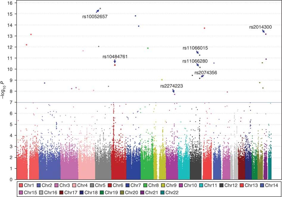
180

181 Candidate Loci and the TDT Often try to map genes by using case/control contrasts, also called association mapping. The frequencies of marker alleles are measured in both a case sample -- showing the trait (or extreme values) control sample -- not showing the trait The idea is that if the marker is in tight linkage, we might expect LD between it and the particular DNA site causing the trait variation. Problem with case-control approach (and association mapping in general): Population Stratification can give false positives. 45 When population being sampled actually consists of several distinct subpopulations we have lumped together, marker alleles may provide information as to which group an individual belongs. If there are other risk factors in a group, this can create a false association btw marker and trait Example. The Gm marker was thought (for biological reasons) to be an excellent candidate gene for diabetes in the high-risk population of Pima Indians in the American Southwest. Initially a very strong association was observed: Gm + Total % with diabetes Present 93 8% Absent 4,67 9% 46

182 Gm + Total % with diabetes Present 93 8% Absent 4,67 9% Problem: freq(gm + ) in Caucasians (lower-risk diabetes Population) is 67%, Gm + rare in full-blooded Pima The association was re-examined in a population of Pima that were 7/8th (or more) full heritage: Gm + Total % with diabetes Present 7 59% Absent,764 6% 47 Linkage vs. Association The distinction between linkage and association is subtle, yet critical Marker allele M is associated with the trait if Cov(M,y) is not While such associations can arise via linkage, they can also arise via population structure. Thus, association DOES NOT imply linkage, and linkage is not sufficient for association 48

183 Transmission-disequilibrium test (TDT) The TDT accounts for population structure. It requires sets of relatives and compares the number of times a marker allele is transmitted (T) versus not-transmitted (NT) from a marker heterozygote parent to affected offspring. Under the hypothesis of no linkage, these values should be equal, resulting in a chi-square test for lack of fit: 49 Scan for type I diabetes in Humans. Marker locus DS5 Allele T NT χ p

184 Accounting for population structure Three classes of approaches proposed ) Attempts to correct for common pop structure signal (genomic control, regression/ PC methods) ) Attempts to first assign individuals into subpopulations and then perform association mapping in each set (Structure) 3) Mixed models that use all of the marker information (Tassle, EMMA, many others) These can also account for cryptic relatedness in the data set, which also causes false-positives. 5 Genomic Control Devlin and Roeder (999). Basic idea is that association tests (marker presence/absence vs. trait presence/absence) is typically done with a standard x χ test. When population structure is present, the test statistic now follows a scaled χ, so that if S is the test statistic, then S/λ ~ χ (so S ~ λχ ) The inflation factor λ is given by Note that this departure from a χ increases with sample size n 5

185 Genomic Control Assume n cases and controls Fraction of cases in kth population λ = + nf ST Σ k (f k -g k ) Population substructure Fraction of controls in kth population Genomic control attempts to estimate λ directly from our distribution of test statistics S 53 Estimation of λ The mean of a χ is one. Hence, since S ~ λχ and we expect most test statistic values to be from the null (no linkage), one estimator of λ is simply the mean of S, the mean value of the test statistics. The problem is that this is not a particular robust estimator, as a few extreme values of S (as would occur with linkage!) can inflate λ over its true value. A more robust estimator is offered from the medium (5% value) of the test statistics, so that for m tests 54

186 Structured Association Mapping Pritchard and Rosenberg (999) proposed Structured Association Mapping, wherein one assumes k subpopulations (each in Hardy- Weinberg). Given a large number of markers, one then attempts to assign individuals to groups using an MCMC Bayesian classifier Once individuals assigned to groups, association mapping without any correction can occur in each group. 55 Regression Approaches A third approach to control for structure is simply to include a number of markers, outside of the SNP of interest, chosen because they are expected to vary over any subpopulations How might you choose these in a sample? Try those markers (read STRs) that show the largest departure from Hardy-Weinberg, as this is expected in markers that vary the most over subpopulations. 56

187 Variations on this theme (eigenstrat) --- use all of the marker information to extract a set of significant PCs, which are then included in the model as cofactors 57 Mixed-model approaches Mixed models use marker data to Account for population structure Account for cryptic relatedness Three general approaches: Treat a single SNP as fixed TASSLE, EMMA Treat a single SNP as random General pedigree method Fit all of the SNPs at once GBLUP 58

188 Structure plus Kinship Methods Association mapping in plants offer occurs by first taking a large collection of lines, some closely related, others more distantly related. Thus, in addition to this collection being a series of subpopulations (derivatives from a number of founding lines), there can also be additional structure within each subpopulation (groups of more closely related lines within any particular lineage). Y = Xβ + Sa + Qv + Zu + e Fixed effects in blue, random effects in red This is a mixed-model approach. The program TASSEL runs this model. 59 Q-K method Y = Xβ + Sa + Qv + Zu + e β = vector of fixed effects a = SNP effects v = vector of subpopulation effects (STRUCTURE) Q ij = Prob(individual i in group j). Determined from STRUCTURE output u = shared polygenic effects due to kinship. Cov(u) = var(a)*a, where the relationship matrix A estimated from marker data matrix K, also called a GRM a genomic relationship matrix 6

189 Which markers to include in K? Best approach is to leave out the marker being tested (and any in LD with it) when construction the genomic relationship matrix LOCO approach leave out one chromosome (which the tested marker is linked to) Best approach seems to be to use most of the markers Other mixed-model approaches along these lines 6 GBLUP The Q-K method tests SNPs one at a time, treating them as fixed effects The general pedigree method (slides 35-36) also tests one marker at a time, treating them as random effects Genomic selection can be thought of as estimating all of the SNP effects at once and hence can also be used for GWAS 6

190 BLUP, GBLUP, and GWAS Pedigree information gives EXPECTED value of shared sites (i.e., ½ for full-sibs) A matrix in BLUP The actual realization of the fraction of shared genes for a particular pair of relatives can be rather different, due to sampling variance in segregation of alleles GRM, genomic relationship matrix (or K or marker matrix M) Hence identical relatives can differ significantly in faction of shared regions Dense marker information can account for this 63 The general setting Suppose we have n measured individuals (the n x vector y of trait values) The n x n relationship matrix A gives the relatedness among the sampled individuals, where the elements of A are obtained from the pedigree of measured individuals We may also have p (>> n) SNPs per individual, where the n x p marker information matrix M contains the marker data, where M ij = score for SNP j (i.e., for, for, for ) in individual i.

191 Covariance structure of random effects A critical element specifying the mixed model is the covariance structure (matrix) of the vector u of random effects Standard form is that Cov(u) = variance component * matrix of known constants This is the case for pedigree data, where u is typically the vector of breeding values, and the pedigree defines a relationship matrix A, with Cov(u) = Var(A) * A, the additive variance times the relationship matrix With marker data, the covariance of random effects are functions of the marker information matrix M. If u is the vector of p marker effects, then Cov(u) = Var(m) * M T M, the marker variance times the covariance structure of the markers. Y = Xβ + Zu + e Pedigree-based BV estimation: (BLUP) u nx = vector of BVs, Cov(u) = Var(A) A nxn Marker-based BV estimation: (GBLUP) u nx = vector of BVs, Cov(u) = Var(m) M T M (n x n) GWAS: u px = vector of marker effects, Cov(u) = Var(m) MM T (p x p) Genomic selection: predicted vector of breeding values from marker effects (genetic breeding values), GBV nx = M nxp u px. Note that Cov(GBV) = Var(m) M T M (n x n) Many variations of these general ideas by adding additional assumptions on covariance structure.

192 GWAS Model diagnostics 67 Genomic control λ as a diagnostic tool Presence of population structure will inflate the λ parameter A value above is considered evidence of additional structure in the data Could be population structure, cryptic relatedness, or both A lambda value less that.5 is generally considered benign One issue is that if the true polygenic model holds (lots of sites of small effect), then a significant fraction will have inflated p values, and hence an inflated λ value. Hence, often one computes the λ following attempts to remove population structure. If the resulting value is below.5, suggestion that structure has been largely removed. 68

193 P P plots Another powerful diagnostic tool is the p-p plot. If all tests are drawn from the null, then the distribution of p values should be uniform. There should be a slight excess of tests with very low p indicating true positives This gives a straight line of a log-log plot of observed (seen) and expected (uniform) p values with a slight rise near small values If the fraction of true positives is high (i.e., many sites influence the trait), this also bends the p-p plot 69 A few tests are significant Great excess of Significant tests Price et al. Nat Rev Gene : 459 7

194 Great excess of Significant tests As with using λ, one should construct p-p following some approach to correct for structure & relatedness to see if they look unusual. 7 Power of Association mapping Q/q is the polymorphic site contributing to trait variation, M/m alleles (at a SNP) used as a marker Let p be the frequency of M, and assume that Q only resides on the M background (complete disequilibrium) Haloptype Frequency effect QM rp a qm (-r)p qm -p 7

195 Haloptype Frequency effect QM rp a qm (-r)p qm -p Effect of m = Effect of M = ar Genetic variation associated with Q = (rp)(-rp)a ~ rpa when Q rare. Hence, little power if Q rare Genetic variation associated with marker M is p(-p)(ar) ~ pa r Ratio of marker/true effect variance is ~ r Hence, if Q rare within the A class, even less power! 73 Common variants Association mapping is only powerful for common variants freq(q) moderate freq (r) of Q within M haplotypes modest to large Large effect alleles (a large) can leave small signals. The fraction of the actual variance accounted for by the markers is no greater than ~ ave(r), the average frequency of Q within a haplotype class Hence, don t expect to capture all of Var(A) with markers, esp. when QTL alleles are rare but markers are common (e.g. common SNPs, p >.5) Low power to detect G x G, G x E interactions 74

196 How wonderful that we have met with a paradox. Now we have some hope of making progress -- Neils Bohr 75 The missing heritability pseudo-paradox A number of GWAS workers noted that the sum of their significant marker variances was much less (typically %) than the additive variance estimated from biometrical methods The missing heritability problem was birthed from this observation. Not a paradox at all Low power means small effect (i.e. variance) sites are unlikely to be called as significant, esp. given the high stringency associated with control of false positives over tens of thousands of tests Further, even if all markers are detected, only a fraction ~ r (the frequency of the causative site within a marker haplotype class) of the underlying variance is accounted for. 76

197 Dealing with Rare Variants Many disease may be influenced by rare variants. Problem: Each is rare and thus overall gives a weak signal, so testing each variant is out (huge multiple-testing problem) However, whole-genome sequencing (or just sequencing through a target gene/region) is designed to pick up such variants Burden tests are one approach Idea: When comparing case vs. controls, is there an overdispersion of mutations between the two categories? 77 Solid = random distribution over cases/controls Blue = observed distribution A: Variants only increase disease risk (excess at high values) B: Variants can both increase (excess high values) and decrease risk (excess low values) --- inflation of the variance 78

198 C(α) test Idea: Suppose a fraction p of the sample are controls, p = -p are cases. Note these varies are fixed over all variants Let n i be the total number of copies of a rare variant i. Under binomial sampling, the expected number of variant i in the case group is ~ Bin(p,n i ) Pool the observations of all such variants over a gene/region of interest and ask if the variance in the number in cases exceeds the binomial sampling variance n i p (-p ) 79 C(α) test (cont). Suppose m variants in a region, test statistic is of the form Σ i (y i - n i p ) - n i p (-p ) y i = number of variant I in cases. This is observed variance minus binomial prediction This is scaled by a variance term to give a test statistic that is roughly normally distributed 8

199 Lecture 9: Using molecular markers to detect selection Bruce Walsh lecture notes Summer Institute in Statistical Genetics Seattle, 3 5 July 5 Detecting selection Bottom line: looking for loci showing departures from the equilibrium neutral model What kinds of selection are of interest? Time scales and questions KEY POINTS False positives very common MOST selective events will not be detected Those that are likely represent a rather biased sample

200 Negative selection is common Negative (or purifying) selection is the removal of deleterious mutations by selection Leaves a strong signal throughout the genome Faster substitution rates for silent vs. replacement codons Comparative genomics equates strong sequence conservation (i.e., high negative selection) with strong functional constraints The search for selection implies selection OTHER than negative 3 Positive selection An allele increasing in frequency due to selection Can either be a new mutation or a previously neutral/slightly deleterious allele whose fitness has changed due to a change in the environment. Adaptation Balancing selection is when alternative alleles are favored by selection when rare MHC, sickle-cell The search for selection is the search for signatures of positive, or balancing, selection 4

201 Time scales of interest Ecological An allele either currently undergoing selection or has VERY recently undergone selection Detect using the nature of genetic variation within a population sample Key: A SINGLE event can leave a signature Evolutionary A gene or codon experiences REPEATED adaptive events over very long periods of time Typically requires between-species divergence data Key: Only informs us as to the long-term PATTERN of selection over a gene 5 6

202 Biased scan for selection Current/very recent selection at a single site requires rather strong selection to leave a signature. Small shifts in allele frequencies at multiple sites unlikely to leave signatures Very small time window (~. Ne generations) to detect such an event once it has occurred. Recurrent selection Phylogenic comparisons: Multiple substitution events at the same CODON required for a signal OK for arms-race genes, likely not typical 7 Recurrent selection at sites OVER a gene Comparing fixed differences between two species with the observed levels of polymorphism Requires multiple substitutions at different codons (i.e., throughout the gene) for any signal Hence, a few CRITICAL adaptive substitutions can occur in a gene and not leave a strong enough signal to detect Power depends on the number of adaptive substitutions over the background level of neutral substitutions 8

203 Sample of a gene from several individuals in the same population * * * * Ongoing, or recent, selection Detecting ongoing selection within a population. Requires a population sample, in which we look for inconsistencies of the pattern of variation from the equilibrium neutral model. Can detect on-going selection in a single region, influencing the pattern of variation at linked neutral loci. 9 Sample of a gene over several species x * *??? Divergence data on a phylogeny. Repeated positive selection at the same site A phylogenic comparison of a sequence over a group of species is done on a codon-by-codon basis, looking for those with a higher replacement than site rate. Requires MULTIPLE substitutions at the same codon over the tree

204 Fixed differences between two species * * * * Positive selection occurring over multiple sites within the gene Comparison of divergence data for a pair of species. Requires a background estimate of the expected divergence from fixation of neutral sites, which is provided from the polymorphism data (I ll cover this shortly). Key points Methods for detecting selection Are prone to false-positives The rejection of the null (equilibrium neutral model) can occur for reasons other the positive/balancing selection, such as changes in the population size Are under-powered Most selection events likely missed Detect only specific types of selection events Ongoing moderate to strong events Repeated adaptive substitutions in a few codons over a phylogeny Repeated adaptive substitutions over all sites in a gene

205 Detecting on-going selection Excessive allele frequency change/divergence Selective Sweeps Reduction in polymorphism around a selected site Shifts in the allele frequency spectrum i.e., too many rare alleles Allelic age inconsistencies Allele too common relative to its age Excessive LD in a common allele 3 Excess allele frequency change Logically, most straightforward Need estimates of N e, time Need two (or more) time points Generally weak power unless selection strong or time between sampling long Example: Divergence between breeds selected for different goals 4

206 5 Five-marker window scans of difference between Holstein & Angus breeds (dairy vs. beef selection) 6

207 Selective sweeps Classic visual tool to look for potential sites under selection Common approach in the search for domestication genes Positive selection reduces Ne for linked sites Reduces TMRCA and hence variation Balancing selection increases Ne for linked sites Increases TMRCA and hence increase variation 7 Past Neutral Selective Sweep Present Balancing selection Longer TMRCA Shorter TMRCA 8

208 Scanning for Sweeps Use a sliding window to look at variation along a chromosome (or around a candidate gene) Decrease (with respect to some standard) consistent with linked site under recent/ ongoing positive selection Increase consistent with balancing selection 9 Signal of positive selection, OR reduction in mutation rate Signal of balancing selection, OR increase in mutation rate

209 Domestication: Maize vs. teosinte tb in maize. Used teosinte as a control for expected background levels of variation

210 ADH in Drosophila. Strong candidate for balancing selection of the Fast and Slow alleles, due to a single aa replacement at the location marked by the arrow 3 Scan of Drosophila genes in Africa (source population) and Europe (recently founded population). Less diversity in Europe, but some loci (filled circles) strong candidates for a sweep 4

211 Double-muscle cattle: Belgian blue 5 Reduction in microsatellite copy number variance often used 6

212 Issues with sweeps Need sufficient background variation before selection for a strong signal Strong domestication event (e.g. sorghum) can remove most variation over entire genome Inbreeding greatly reduces variation The signal persists for only a short time ~. Ne generations Distance for effects roughly. s/c Sweep region often asymmetric around target site Hard sweeps can be detected, soft sweeps leave (at best) a weak signal 7 A) Hard Sweep B) Soft Sweep Rapid fixation under selection Rapid fixation under selection Selection starts at the appearance the new mutation drift & mutation Initially, new mutation is neutral 8

213 Site frequency spectrum tests A large collection of tests based on comparing different measures of variation at a target site within a population sample Tajima s D is the classic Problem: significant result from either selection OR changes in population size/ structure (drift, mutation NOT at equilibrium) 9 Under the equilibrium neutral model, multiple ways to estimate θ = 4N e u using different metrics of variation All should be consistent if model holds. 3

214 Tajima s D Negative value: excess number of rare alleles consistent with either positive selection OR expanding population size Positive value: excess number of common alleles consistent with either balancing selection OR Population subdivision 3 Consistency of allelic age Age/N Under drift, a common allele is an old allele Allele frequency Common alleles should not be young 3

215 33 Starting haplotype freq time Common alleles should have short haplotypes under drift -- longer time for recombination to act Common alleles with long haplotypes --- good signal for selection, rather robust to demography 34

216 Joint polymorphism-divergence tests HKA, McDonald-Kreitman (MK) tests MK test is rather robust to demographic issues Require polymorphism data from one (or more) species, divergence data btw species Look at ratio of divergence to polymorphism 35 Cool feature: can estimate # of adaptive substitutions = 7-7(/4) = 6 Robust to most demographic issues However, replacement polymorphic sites can overestimate neutral rate due to deleterious alleles segregating 36

217 Strengths and weaknesses Only detects a pattern of adaptive substitutions at a gene. Require multiple events to have any power Can t tell which replacements were selectivelydriven MK test robust to many demographic issues, but NOT fool-proof Any change in the constraints between processes generating polymorphisms and processes generating divergence can be regarded as evidence for selection 37 38

218 K A /K s tests THE classic test for selection, requiring gene sequences over a known phylogeny K A = replacement substitution rate K s = silent substitution rate Neutral proxy ω = K A /K s ω > : positive selection. Problem: most codons have K s > K A, so that even with repeated adaptive substitutions throughout a gene, signal still swamped. 39 4

219 Codon-based models The way around this problem is to analyze a gene on a codon-by-codon basis Such codon-based models assign all (nonstop) codons a value from to 6 A model of transition probabilities between all one-nucleotide transitions is constructed Maximum likelihood used to estimate parameters Model with ω = over all codons contrasted with a model where ω > at some (unspecified) set of codons. 4 4

220 Model easily expanded to allow for several classes of codons Can use Baye s theorem to assign posterior probabilities that a given codon is in a given class (i.e., localize sites of repeated positive selection 43 44

221 45 Strengths and weaknesses Strengths Can assign repeated selection to SPECIFIC codons Requires only single sequences for each species Weaknesses: Models can be rather delicate Can only detect repeated selection at particular codons, NOT throughout a gene 46

222 The spandrels of San Marco (Gould and Lewontin 979) Very elaborate structure DOES not imply function nor adaptation 47 Structure vs. function Molecular biologists are largely conditioned to look for function through structure Problem: elaborate structures can serve little function Cannot simply assume an adaptive explanation because the structure is complex 48

223 49 ω values shown on braches ASPM 5

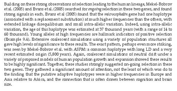
224 5 5