Numerical Integration and Numerical Differentiation. Hsiao-Lung Chan Dept Electrical Engineering Chang Gung University, Taiwan

Transcription

1 Numerical Integration and Numerical Differentiation Hsiao-Lung Chan Dept Electrical Engineering Chang Gung University, Taiwan

2 Integration 2

3 Mean for discrete and continuous data Discrete data Continuous data 3

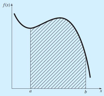
4 Numerical integration, also referred to as quadrature The integral may be evaluated over a line, an area, or a volume Determine the net force due to a non-uniform wind blowing against the side of a skyscraper Areal integral: Compute the total rate of energy transfer across a plane where the flux is a function of position Volume integral: the total mass of chemical contained in a reactor is given as the product of the concentration of chemical and the reactor volume. 4

5 Newton-Cotes formulas The strategy of replacing a complicated function or tabulated data with a polynomial that is easy to integrate I b f x dx f n x dx a b a The approximation of an integral by the area under a straight line and a parabola 5

6 Trapezoidal rule The first of the Newton-Cotes closed integration formulas b I f n x dx I a b f (a) f b f a x a dx a b a I b a f a f b 2 6

7 Composite trapezoidal rule x n x 1 x 2 x n I f n x dx f n x dx f n x dx f n x dx x 0 I x 1 x 0 f x 0 f x 1 2 I h n 1 2 f x 0 2 f x i f x n i 1 x 0 x 1 x 2 x 1 f x 1 f x 2 2 x n 1 x n x n 1 f x n 1 f x n 2 7

8 M-file to implement the composite trapezoidal rule function I = trap(func,a,b,n,varargin) % a, b = integration limits, n = number of segments if nargin<3, error('at least 3 input arguments required'), end if ~(b>a), error('upper bound must be greater than lower'), end if nargin<4 isempty(n), n=100; end x = a; h = (b - a)/n; s=func(a,varargin{:}); for i = 1 : n-1 x = x + h; s = s + 2*func(x,varargin{:}); end s = s + func(b,varargin{:}); I = (b - a) * s/(2*n); 8

9 Example: Determine the distance fallen by the free-falling bungee jumper Falling velocity v t gm c d tanh gc m d t If g = 9.81 m/s2,m = 68.1 kg, cd = 0.25 kg/m, determine falling distance in the first 3 s v=@(t) sqrt(9.81*68.1/0.25)*tanh(sqrt(9.81*0.25/68.1)*t) falldist=trap(v,0,3,5); 9

10 Simpson s rules A more accurate estimate of an integral Apply the trapezoidal rule with finer segmentation Use higher-order polynomials to connect the points Simpson s 1/3 Rule using a 2 nd -order Lagrange polynomial 10

11 Composite Simpson s 1/3 rule 11

12 Simpson s 3/8 rule A third-order Lagrange polynomial is fit to four points and integrated to yield Simpson s 1/3 rule Simpson s 3/8 rule 12

13 Higher-order newton-cotes formulas 13

14 Integration with unequal segments Apply the trapezoidal rule M-file for implementing the trapezoidal rule for unequally spaced data x = [ ]; y = *x-200*x.^2+675*x.^3-900*x.^4+400*x.^5; z= trapuneq(x,y); 14

15 M-file to implement the trapezoidal rule for unequally spaced data function I = trapuneq(x,y) if nargin<2, error('at least 2 input arguments required'),end if any(diff(x)<0), error('x not monotonically ascending'),end n = length(x); if length(y)~=n, error('x and y must be same length'); end s = 0; for k = 1:n-1 s = s + (x(k+l)-x(k))*(y(k)+y(k+l))/2; end I = s; 15

16 MATLAB s built-in function for evaluating integrals z = trapz(x, y) x = [ ]; y = *x-200*x.^2+675*x.^3-900*x.^4+400*x.^5; z = trapz(x,y); z = cumtrapz(x, y) Computes the cumulative integral z = a vector whose elements z(k) hold the integral from x(1) to x(k) Cumulative integral 16

17 Multiple integrals Double integral 17

18 MATLAB s built-in function of multiple integral Double (dblquad) and triple (triplequad) integration q = dblquad(fun, xmin, xmax, ymin, ymax, tol); tol: a default tolerance of is used Example: the temperature of a rectangular heated plate is described by the following function q = dblquad(@(x,y) 2*x*y+2*x-x.^2-2*y.^2+72,0,8,0,6); 18

19 Definition of a derivative Difference approximation Derivative x approaches zero 19

20 High-accuracy differentiation formulas Taylor series expansion can be used to generate highaccuracy formulas for derivatives Forward finite-difference Backward finite-difference Centered finite-difference 20

21 High-accuracy differentiation formulas (cont.) Forward Taylor series expansion Substitute into the above equation Improve the accuracy to O(h 2 ). 21

22 High-accuracy differentiation formulas (cont.) Forward finite-difference formulas Backward finite-difference formulas Centered finite-difference formulas 22

23 MATLAB built-in function of derivative: diff *x-200*x.^2+675*x.^3-900*x.^4+400*x.^5; x=0:0.1:0.8; y=f(x); % generate a series of equally spaced values of variables % numerical estimate of differentiation d=diff(y)./diff(x); d=diff(f(x))/0.1; % because of equally spaced values % analytical estimate of differentiation xa=0:.01:.8; ya=25-400*xa+3*675*xa.^2-4*900*xa.^3+5*400*xa.^4; n=length(x); xm=(x(1:n-1)+x(2:n))./2; plot(xm,d,'o',xa,ya) 23

24 MATLAB built-in function diff (cont.) 24

25 MATLAB built-in function of derivative: gradient *x-200*x.^2+675*x.^3-900*x.^4+400*x.^5; x=0:0.1:0.8; y=f(x); % generate a series of equally spaced values of variables % numerical estimate of differentiation dy=gradient(y,0.1); % because of equally spaced values % analytical estimate of differentiation xa=0:.01:.8; ya=25-400*xa+3*675*xa.^2-4*900*xa.^3+5*400*xa.^4; n=length(x); xm=(x(1:n-1)+x(2:n))./2; plot(xm,d,'o',xa,ya) 25

26 MATLAB built-in function gradient (cont.) centered differences for intermediate values forward and backward differences at the ends 26

27 Partial derivatives Partial first derivatives can be approximated with centered differences 27

28 Example: gradient of mountain elevation z = f (x, y) where z = elevation, x = distance measured along the eastwest axis, y = distance measured along the north-south axis. The gradient of f(x,y) which represents the steepest Slope with a magnitude and direction 28

29 Gradient of mountain elevation (cont.) y-x-2*x.^2-2.*x.*y-y.^2; [x,y]=meshgrid(-2:.25:0, 1:.25:3); z=f(x,y); [fx,fy]=gradient(z,0.25); cs=contour(x,y,z); clabel(cs); hold on % Resultant of partial derivatives is % superimposed as vectors on contour plot quiver(x,y,-fx,-fy); hold off 29

30 Reference Steven C. Chapra "Applied Numerical Methods with MATLA B", 3rd ed., McGraw Hill,