EAD 115. Numerical Solution of Engineering and Scientific Problems. David M. Rocke Department of Applied Science

Transcription

1 EAD 115 Numerical Solution of Engineering and Scientific Problems David M. Rocke Department of Applied Science

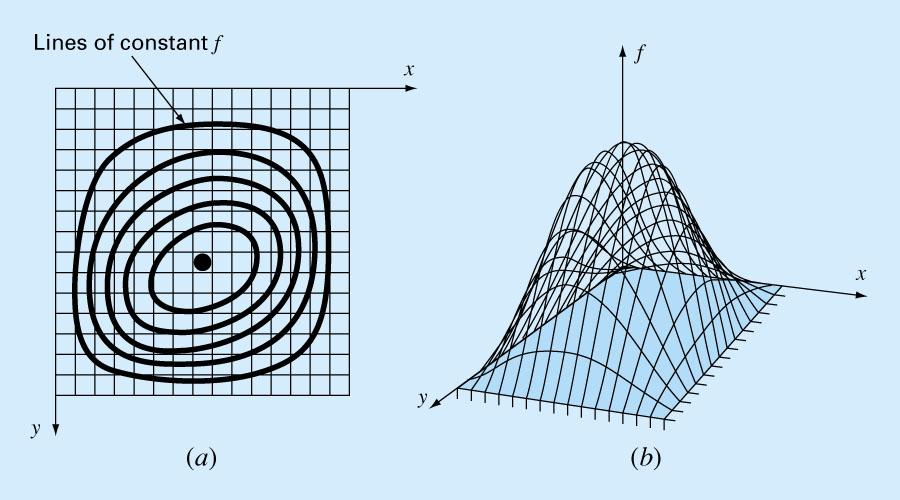
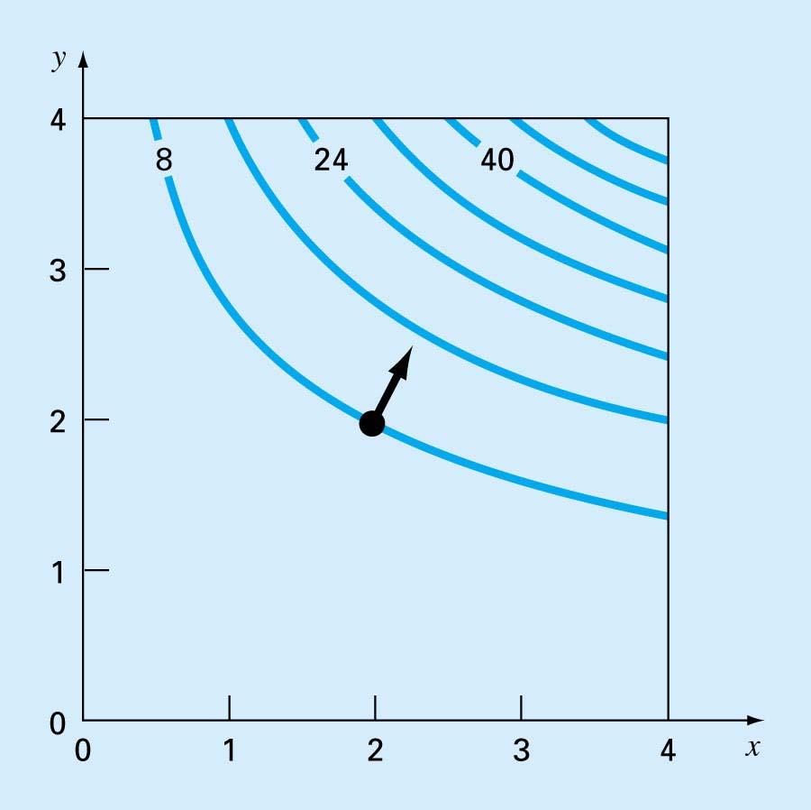
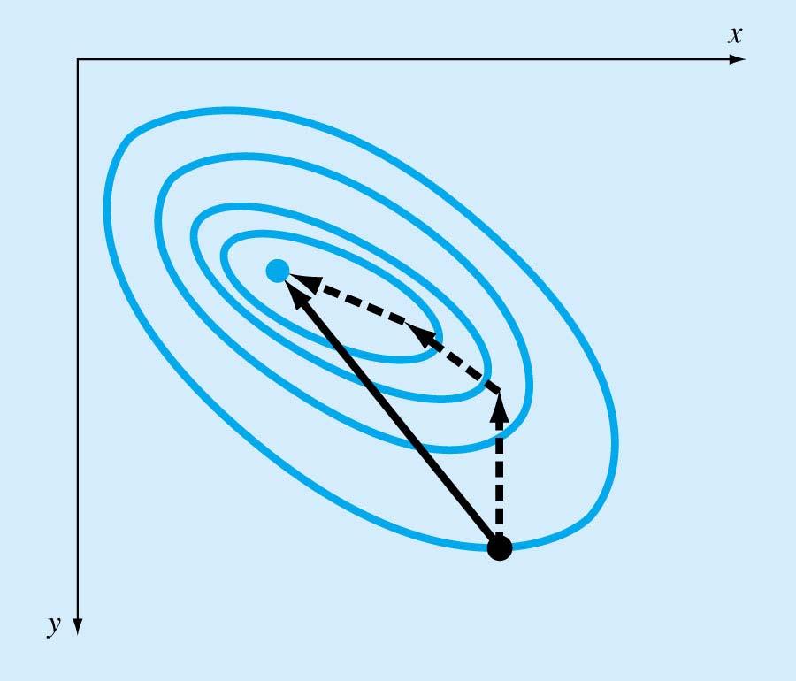
2 Multidimensional Unconstrained Optimization Suppose we have a function f() of more than one variable f(x 1, x 2,, x n ) We want to find the values of x 1, x 2,, x n that give f() the largest (or smallest) possible value Graphical solution is not possible, but a graphical picture helps understanding Hilltops and contour maps

3

4 Methods of solution Direct or non-gradient methods do not require derivatives Grid search Random search One variable at a time Line searches and Powell s method Simplex optimization

5 Gradient methods use first and possibly second derivatives Gradient is the vector of first partials Hessian is the matrix of second partials Steepest ascent/descent Conjugate gradient Newton s method Quasi-Newton methods

6 Grid and Random Search Given a function and limits on each variable, generate a set of random points in the domain, and eventually choose the one with the largest function value Alternatively, divide the interval on each variable into small segments and check the function for all possible combinations

7 Features of Random and Grid Slow and inefficient Search Requires knowledge of domain Works even for discontinuous functions Poor in high dimension Grid search can be used iteratively, with progressively narrowing domains

8 Line searches Given a starting point and a direction, search for the maximum, or for a good next point, in that direction. Equivalent to one dimensional optimization, so can use Newton s method or another method from previous chapter Different methods use different directions

9 x v ( x, x,, x ) 1 2 ( v, v,, v ) 1 2 n n f( x) f( x, x,, x ) 1 2 gλ( ) f ( x λ v) n

10 One-Variable-at-a Time Search Given a function f() of n variables, search in the direction in which only variable 1, changes Then search in the direction from that point in which only variable 2 changes, etc. Slow and inefficient in general Can speed up by searching in a direction after n changes (pattern direction)

11

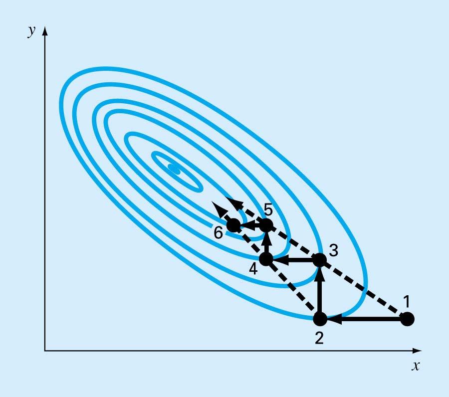
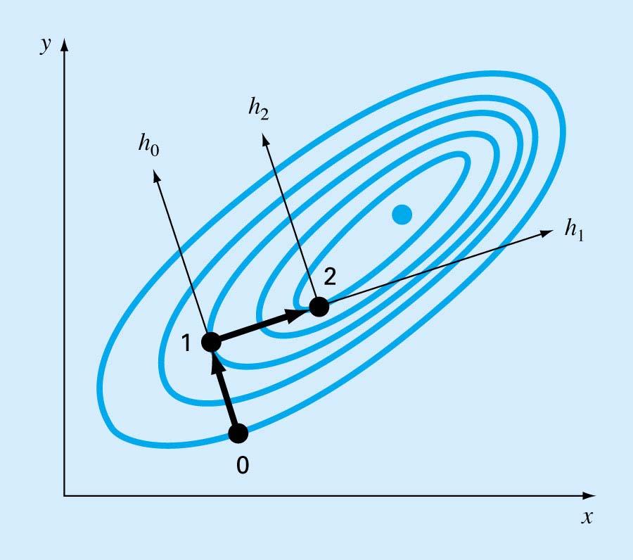
12 Powell s Method If f() is quadratic, and if two points are found by line searches in the same direction from two different starting points, then the line joining the two ending points (a conjugate direction) heads toward the optimum Since many functions we encounter are approximately quadratic near the optimum, this can be effective

13

14 Start with a point x 0 and two random directions h 1 and h 2 Search in the direction of h 1 from x 0 to find a new point x 1 Search in the direction of h 2 from x 1 to find a new point x 2. Let h 3 be the direction joining x 0 to x 2 Search in the direction of h 3 from x 2 to find a new point x 3 Search in the direction of h 2 from x 3 to find a new point x 4 Search in the direction of h 3 from x 4 to find a new point x 5

15 Points x 3 and x 5 have been found by searching in the direction of h 3 from two starting points x 2 and x 4 Call the direction joining x 3 and x 5 h 4 Search in the direction of h 4 from x 5 to find a new point x 6 The new point x 6 will be exactly the optimum if f() is quadratic The iterations can then be repeated Errors estimated by change in x or in f()

16

17 Nelder-Mead Simplex Algorithm Direct search method that uses simplices, which are triangles in dimension 2, pyramids in dimension 3, etc. At each iteration a new point is added usually in the direction of the face of the simplex with largest function values

18

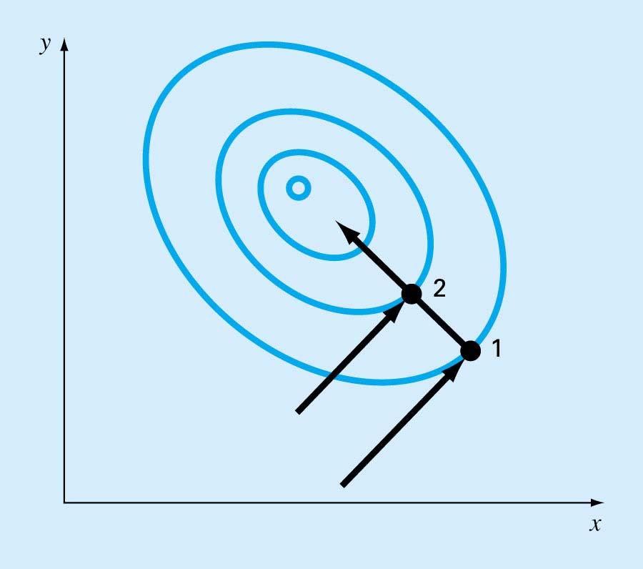
19 Gradient Methods The gradient of f() at a point x is the vector of partial derivatives of the function f() at x For smooth functions, the gradient is zero at an optimum, but may also be zero at a non-optimum The gradient points uphill The gradient is orthogonal to the contour lines of a function at a point

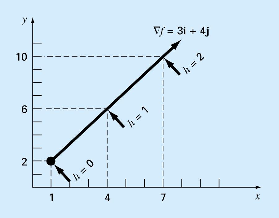
20 Directional Derivatives Given a point x in R n, a unit direction v, and a function f() of n variables, we can define a new function g() of one variable by g(λ)=f(x+λv) The derivative g (λ) is the directional derivative of f() at x in the direction of v This is greatest when v is in the gradient direction

21 x v ( x, x,, x ) 1 2 ( v, v,, v ) T 1 vv 1 2 i 1 2 i f( x) f( x, x,, x ) 1 2 f f f f,,, x x x 1 2 gλ( ) f ( x λ v) n v n n n T f f f g'(0) ( f) v v, v,, vn x x x n n

22 Steepest Ascent The gradient direction is the direction of steepest ascent, but not necessarily the direction leading directly to the summit We can search along the direction of steepest ascent until a maximum is reached Then we can search again from a new steepest ascent direction

23 xx f( x, x) at (2,2) f (2,2) f ( x, x ) x f (2,2) 4 f ( x, x) 2 xx f (2,2) f (2,2) (4,8) (2 4 λ,2 8 λ) is the gradient line gλ( ) f (2 4 λ,2 8 λ ) (2 4 λ )(2 8 λ ) 2

24

25

26 The Hessian The Hessian of a function f() is the matrix of second partial derivatives The gradient is always 0 at a maximum (for smooth functions) The gradient is also 0 at a minimum The gradient is also 0 at a saddle point, which is neither a maximum nor a minimum A saddle point is a max in at least one direction and a min in at least one direction

27

28 Max, Min, and Saddle Point For one-variable functions, the second derivative is negative at a maximum and positive at a minimum For functions of more than one variable, a zero of the gradient is a max if the second directional derivative is negative for every direction and is a min if the second directional derivative is positive for every direction

29 Positive Definiteness A matrix H is positive definite if x T Hx > 0 for every vector x Equivalently, every eigenvalue of H is positive λ is an eigenvalue of H with eigenvector x if Hx = λx -H is positive definite if every eigenvalue of H is negative

30 Max, Min, and Saddle Point If the gradient f of a function f is zero at a point x and the Hessian H is positive definite at that point, then x is a local min If f is zero at a point x and -H is positive definite at that point, then x is a local max If f is zero at a point x and neither H nor -H is positive definite at that point, then x is a saddle point The determinant H helps only in dimension 1 or 2

31 Steepest Ascent/Descent This is the simplest of the gradient-based methods From the current guess, compute the gradient Search along the gradient direction until a local max is reached of this onedimensional function Repeat until convergence

32

33 Eigenvalues Suppose the gradient is 0 and H is the Hessian H is positive definite if and only if all the eigenvalues of H are positive (minimum). -H is positive definite if and only if all the eigenvalues of H are negative (maximum). If the eigenvalues of H are not all of the same sign then we have a saddle point.

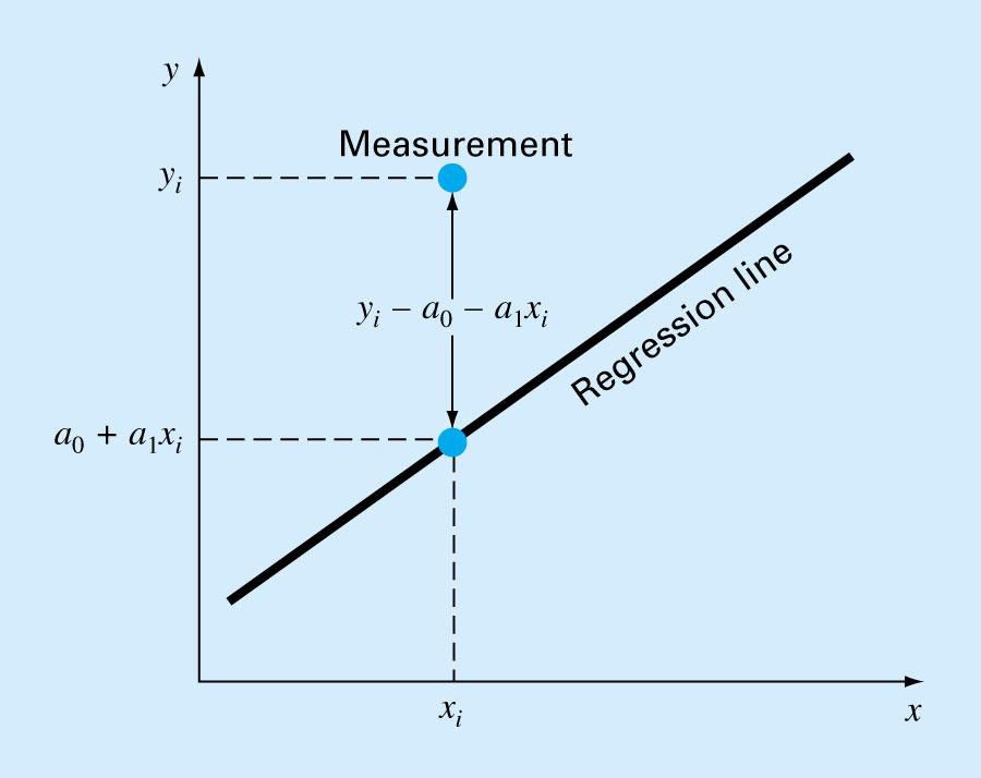
34 Practical Steepest Ascent In real examples, the maximum in the gradient direction cannot be calculated analytically Problem reduces to one dimensional optimization as a line search One can also use more primitive line searches that are fast but do not try to find the absolute optimum

35 Newton s Method Steepest ascent can be quite slow Newton s method is faster, though it requires evaluation of the Hessian Function is modeled by a quadratic at a point using first and second derivatives The quadratic is solved exactly This is used as the next iterate

36 A second-order multivariate Taylor series expansion at the current iterate is T T f( x) = f( x ) + f ( x )( x x ) + 0.5( x x ) H ( x x ) i i i i i i At the optimum, the gradient is 0, so f( x) = f( x ) + H ( x x ) = 0 i i i If H is invertible,then 1 x = i+ 1 x i H i f( xi) In practice, solve the linear problem, H x= H x f( x ) i i i i

37

38 Curve Fitting Given a set of n points (x i, y i ), find a fitted curve that provides a fitted value y = f(x) for each value of x in a range. The curve may interpolate the points (go through each one), either linearly or nonlinearly, or may approximate the points without going through each one, as in least-squares regression.

39

40

41 Simple Linear Regression We have a set of n data points, each of which has a measured predictor x and a measured response y. We wish to develop a prediction function f(x) for y. In the simplest case, we take f(x) to be a linear function of x, as in f(x) = a 0 + a 1 x

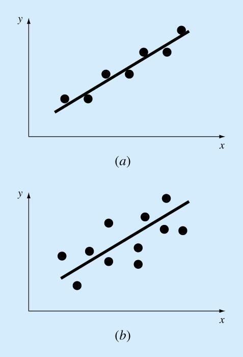
42 Criteria and Estimation If we have one point, way (1,1), then many lines fit perfectly: f(x) = x, f(x) = 2x-1 f(x) = -x+2 If there are two points, say (1,1) and (2,3), then in general there is exactly one line going through the points: f(x) = 2x-1.

43 If there are more than two points, then in general there is no straight line through all of them. These problems are, respectively, underdetermined, determined, and overdetermined. Reasonable criteria for choosing the coefficients a and b in f(x) = a 0 + a 1 x lie in minimizing the size of the residuals: r i = y i f(x i ) = y i (a 0 + a 1 x i ), but how to combine different residuals?

44

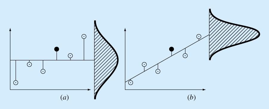
45 The least-squares criterion minimizes n n 2 i i i i= 1 i= 1 = = ( ( )) 2 SS r y f x There are many other possible criteria. Use of the least-squares criterion does not imply any beliefs about the data Use of the linear form for f(x) assumes that this straight-line relationship is reasonable Assumptions are needed for inference about the predictions or about the relationship itself

46 Mininimize Sum of Residuals Minimize Sum of Absolute Values of Residuals Minimize Max Residual

47 Computing the Least-Squares Solution We wish to minimize the sum of squares of deviations from the regression line by choosing the coefficients a 0 and a 1 accordingly Since this is a continuous, quadratic function of the coefficients, one can simply set the partial derivatives equal to zero

48 n n n 2 ( ( )) = i = i i = ( i 0 1 i) i= 1 i= 1 i= 1 SS( a, a ) r y f x y a a x SS( a, a ) n n n n 0 1 0= = 2 ( yi a0 ax 1 i) = 2 yi a0 ax 1 i a 0 i= 1 i= 1 i= 1 i= 1 SS( a, a ) n n n n = = 2 ( yi a0 ax 1 i) xi = 2 xy i i ax 0 i ax 1 i a 1 i= 1 i= 1 i= 1 i= 1 na + a x 0 1 n i= 1 i = i= 1 n n n 2 0 i 1 i = i i i= 1 i= 1 i= 1 a x a x xy n y i

49 These normal equations have a unique solution as two equations in two unknowns The straight line that is calculated in this way is used in practice to see if there is a relationship between x and y It is also used to predict y from x It can also be used to predict x from y by inverting the equation We now look at some practical uses of least squares

50 Quantitative Prediction Regression analysis is the statistical name for the prediction of one quantitative variable (fasting blood glucose level) from another (body mass index) Items of interest include whether there is in fact a relationship and what the expected change is in one variable when the other changes

51 Assumptions Inference about whether there is a real relationship or not is dependent on a number of assumptions, many of which can be checked When these assumptions are substantially incorrect, alterations in method can rescue the analysis No assumption is ever exactly correct

52 Linearity This is the most important assumption If x is the predictor, and y is the response, then we assume that the average response for a given value of x is a linear function of x E(y) = a + bx y = a + bx + ε ε is the error or variability

53

54

55 In general, it is important to get the model right, and the most important of these issues is that the mean function looks like it is specified If a linear function does not fit, various types of curves can be used, but what is used should fit the data Otherwise predictions are biased

56 Independence It is assumed that different observations are statistically independent If this is not the case inference and prediction can be completely wrong There may appear to be a relationship even though there is not Randomization and control prevents this in general

57

58

59 Note no relationship between x and y These data were generated as follows: x y x y 0.95x i 1 i i 0.95y ε η i 1 i i

60 Constant Variance Constant variance, or homoscedacticity, means that the variability is the same in all parts of the prediction function If this is not the case, the predictions may be on the average correct, but the uncertainties associated with the predictions will be wrong Heteroscedacticity is non-constant variance

61

62

63 Consequences of Heteroscedacticity Predictions may be unbiased (correct on the average) Prediction uncertainties are not correct; too small sometimes, too large others Inferences are incorrect (is there any relationship or is it random)

64 Normality of Errors Mostly this is not particularly important Very large outliers can be problematic Graphing data often helps If in a gene expression array experiment, we do 40,000 regressions, graphical analysis is not possible Significant relationships should be examined in detail

65

66 Example Analysis Standard aqueous solutions of fluorescein (in pg/ml) are examined in a fluorescence spectrometer and the intensity (arbitrary units) is recorded What is the relationship of intensity to concentration? Use later to infer concentration of labeled analyte

67 concen~n intens~y

68 intensity concentration

69 . regress intensity concentration Source SS df MS Number of obs = F( 1, 5) = Model Prob > F = Residual R-squared = Adj R-squared = Total Root MSE = intensity Coef. Std. Err. t P> t [95% Conf. Interval] concentrat~n _cons

70 . regress intensity concentration Source SS df MS Number of obs = F( 1, 5) = Model Prob > F = Residual R-squared = Adj R-squared = Total Root MSE = intensity Coef. Std. Err. t P> t [95% Conf. Interval] concentrat~n _cons Slope

71 . regress intensity concentration Source SS df MS Number of obs = F( 1, 5) = Model Prob > F = Residual R-squared = Adj R-squared = Total Root MSE = intensity Coef. Std. Err. t P> t [95% Conf. Interval] concentrat~n _cons Intercept = intensity at zero concentration

72 . regress intensity concentration Source SS df MS Number of obs = F( 1, 5) = Model Prob ANOVA > F = Residual R-squared = Adj Table R-squared = Total Root MSE = intensity Coef. Std. Err. t P> t [95% Conf. Interval] concentrat~n _cons

73 . regress intensity concentration Source SS df MS Number of obs = F( 1, 5) = Model Prob > F = Residual R-squared = Adj R-squared = Total Root MSE = intensity Coef. Std. Err. t P> t [95% Conf. Interval] concentrat~n Test of overall model _cons

74 . regress intensity concentration Source SS df MS Number of obs = F( 1, 5) = Model Prob > F = Residual R-squared = Adj R-squared = Total Root MSE = intensity Coef. Std. Err. t P> t [95% Conf. Interval] concentrat~n Variability around the regression line _cons

75 concentration intensity Fitted values

76 Residuals Fitted values

77 Use of the calibration curve yˆ x yˆ is the predicted average intensity x is the true concentration y 1.52 xˆ 1.93 y is the observed intensity xˆ is the estimated concentration

78

79 Measurement and Calibration Essentially all things we measure are indirect The thing we wish to measure produces an observed transduced value that is related to the quantity of interest but is not itself directly the quantity of interest Calibration takes known quantities, observes the transduced values, and uses the inferred relationship to quantitate unknowns

80 Measurement Examples Weight is observed via deflection of a spring (calibrated) Concentration of an analyte in mass spec is observed through the electrical current integrated over a peak (possibly calibrated) Gene expression is observed via fluorescence of a spot to which the analyte has bound (usually not calibrated)

81 Measuring Variation If we do not use any predictor, the variability of y is its variance, or mean square difference between y and the mean of all the y s. If we use a predictor, then the variability is the mean square difference between y and its prediction

82

83

84 n 1 2 MST = n 1 y y ( ) ( ) i= 1 ( ) ( ) ( ) i 0 1 i ( ) ( ) ( ) n 1 2 MSE = n 2 y yˆ 1 i= 1 n = n 2 y a ax i= 1 MSR = SST SSE i i /1 i 2

85 concentration intensity Fitted values

86 Source SS df MS Model Residual Total

87 Multiple Regression If we have more than one predictor, we can still fit the least-squares equations so long as we don t have more coefficients than data points This involves solving the normal equations as a matrix equation

88 y = xb + ε Y = XB + E n = number of data points p = number of predictors including constant y is 1 1 x is 1 p B is p 1 ε is 1 1 Y is n 1 X is n p E is n 1

89 Y = XB + E n = number of data points p = number of predictors including constant B is p 1 Y is n 1 X is n p E is n 1 ( Y XBˆ ) is n 1 ( Y XBˆ) ( Y XBˆ) is 1 1, the SSE

90 ( Y XBˆ) ( Y XBˆ) is 1 1, the SSE To minimize this over choices of B, solve ( XX ) Bˆ = ( XY ) ˆ 1 = ( ) ( ) B XX XY

91 Linearization of Nonlinear Relationships We can fit a curved relationship with a polynomial The relationship f(x) = a 0 + a 1 x + a 2 x 2 can be treated as a problem with two predictors This can then be dealt with as any multiple regression problem

92 Sometimes a nonlinear relationship can be linearized by a transformation of the response and the predictor Often this involves logarithms, but there are many possibilities

93 y ln y y = αe β x = lnα + βx d a = a+ 1 + / d a = 1 + / y a d y b = ( x/ c) y a ( x c) ( x c) d y ln = bln c+ bln x y a b b

94

95 Intrinsic nonlinearity We can still solve the least-squares problem even if f(x) is not linear in the parameters We do this by approximate linearization at each step = Gauss-Newton There are other, more effective methods, but this is beyond our scope

96 y = f( x; a, a, a ) + ε i i 0 1 n ( a x ) 1, j 1, j ( ax) 1 ( ) ( ) 0( j) + 0( j) 0 0, j + 1( ( ) j) a1 a1, j ( ) y = f( x; a, a, a ) + f ( x; a, a, a ) a a + i i 0, j 1, j n, j 0 i 0, j 1, j n, j 0 0, j 0 + f ( x; a, a, a ) a a + ε 1 j 0, j j n i 0, j 1, j n, j n n, j y = f( x) + ε = a 1 e + ε f ( x ) = 1 e j f( x) = a xe 0 a y f x f x a a f x y f ( x ) f ( x ) a + f ( x ) a j x j 0 j 0 j 0 1 j 1 Solve for a and a by linear least squares. 0 1 Repeat until convergence.

97 Interpolation Given a set of points (x i, y i ), an interpolating function is one which is defined for all x in the range of the x i, and which satisfies f(x i ) = y i. Polynomials are a convenient class of functions to use for this purpose, though others such as splines are also used. There are different ways to express the same polynomial. Given n points, we can in general determine an n-1 degree polynomial that interpolates them.

98 Linear function Two points Degree one Quadratic function Three points Degree Two Cubic function Four points Degree three

99 Linear Interpolation

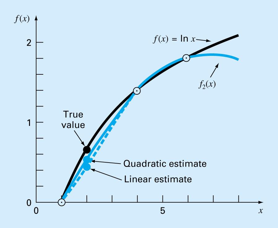
100 f x f x f x f x = x x x x ( ) ( ) ( ) ( ) ( ) ( ) f x f x f x = f x + x x ( ) ( ) 1 0 ( ) x1 x0 ln(1) = 0 ln(4) = ln( x) f1( x) = 0 + ( x 1) ln(2) f1(2) = (2 1) = ln(2) =

101

102 Quadratic Interpolation Three points determine a quadratic This should fit many functions better than linear interpolation We derive a general form for quadratic interpolation We then derive a method to estimate the three unknowns (coefficients) that determine a quadratic function

103

104 f ( x) = b + b( x x ) + b ( x x )( x x ) = b + bx bx + bx + bxx bxx bxx which is of the form = a + ax+ ax with a = b bx + bx x a = b bx bx a = b which shows either form is general

105 f ( x) = b + b( x x ) + b ( x x )( x x ) f( x ) b b f( x ) f( x ) = b + b( x x ) f( x ) = f( x ) + b( x x ) b = = = f( x1) f( x0) ( x x ) 1 0

106 f ( x) = b + b( x x ) + b ( x x )( x x ) b b f( x ) f( x1) f( x0) ( x x ) 1 0 f( x ) f( x ) f( x ) = f( x ) + ( x x ) + b ( x x )( x x ) ( x1 x0) f( x2) f( x0) f( x1) f( x0) ( x2 x0) = + b ( x x )( x x ) ( x x ) ( x x )( x x ) b = = f( x ) f( x ) f( x ) f( x ) ( x x )( x x ) ( x x )( x x ) =

107 b b b b b b f( x2) f( x0) f( x1) f( x0) = ( x x )( x x ) ( x x )( x x ) f( x2) f( x1) f( x1) f( x0) f( x1) f( x0) = + ( x x )( x x ) ( x x )( x x ) ( x x )( x x ) = + [ f( x ) f( x )][( x x ) ( x x )] f( x ) f( x ) ( x2 x0)( x2 x1) ( x2 x0)( x2 x 1 )( x 1 x 0 ) f( x2) f( x1) f( x1) f( x0) = ( x x )( x x ) ( x x )( x x ) = = f( x2) f( x1) f( x1) f( x0) ( x2 x1) ( x1 x0) ( x x ) 2 0 f( x2) f( x1) f( x1) f( x0) ( x2 x1) ( x1 x0) ( x x )

108 f ( x) = b + b( x x ) + b ( x x )( x x ) b b f( x ) f( x1) f( x0) ( x x ) 1 0 looks like a finite first divided difference b = = = f( x2) f( x1) f( x1) f( x0) ( x2 x1) ( x1 x0) ( x x ) 2 0 looks like a finite second divided difference

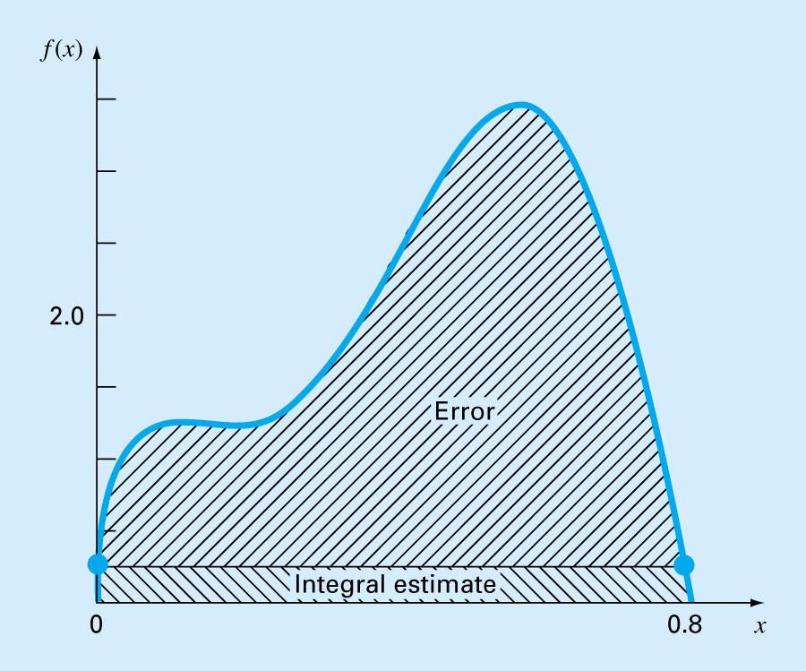
109 Approximate ln(2) = by interpolating (1, 0) (4, ) (6, ) b b b = f( x ) = 0 = f( x1) f( x0) = = ( x x ) ( 2) f( x1) f( x1) f( x0) x2 x1 x1 x0 f x ( ) ( ) = ( x x ) = f ( x) = b + b( x x ) + b ( x x )( x x ) f (2) = (2 0) (2 0)(2 4) = =

110 General Form of Newton s Divided Difference Interpolating Polynomials The order n polynomial interpolates n+1 points The coefficients are finite divided differences They can be calculated recursively

111 f ( x) = b + b( x x ) + b( x x )( x x ) + + b ( x x )( x x ) ( x x ) b b n n 0 1 n = f( x ) 0 0 = f[ x, x ] b = f[ x, x, x ] b = f[ x, x,, x, x ] n n n f[ x, x,, x, x ] = i i f[ xi, xi 1,, x2, x1] f[ xi 1, xi 2,, x1, x0] x x i 0

112

113 xi f(xi) 1st dd 2nd dd 3rd dd 4th dd

114 Lagrange Interpolating Polynomial Given n+1 points and function values, there is only one degree-n polynomial going through the points The Lagrange formulation is thus equivalent, leading to the same interpolating polynomial It is easier to calculate

115 f ( x) = L( x) f( x ) n i i i= 0 L( x) i n n j= 0 i j j i This passes through each of the points because when x = x, all of the L( x) are 0 except for L k = k x x x ( x), which is equal to 1. x j i

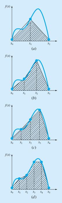
116 Numerical Integration Some functions of known form can be integrated analytically Others require numerical estimates because the form of the integrand yields no closed form solution Sometimes the function may not even be defined by an equation, but rather by a computer program

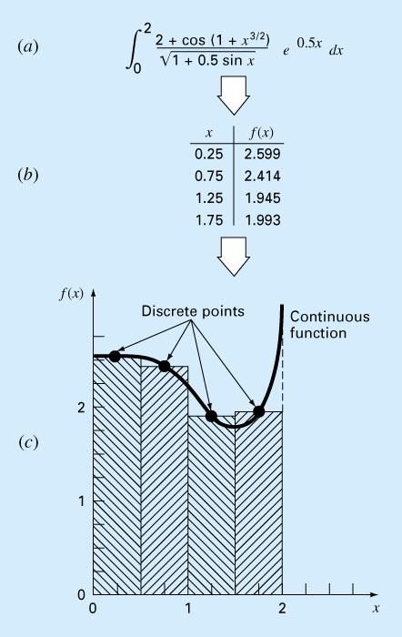
117 0 π x dx /2 π /2 4 2 x = = = sin( x) dx = cos( x) 1 0 = cos( π / 2) + cos(0) = 0+ 1= e x 2 dx =?

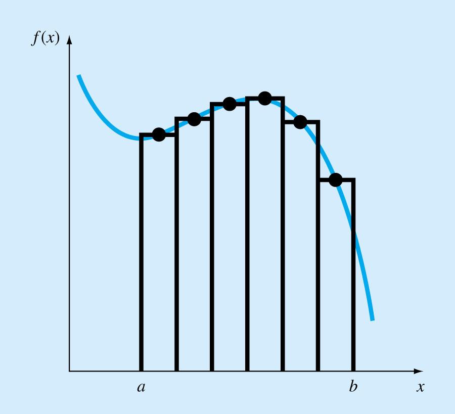
118 Left and right Riemann sums, and the midpoint rule give definition, not a good computational method. Exact only for constant functions (LR and RR) or linear functions (MR). The Definite Integral b a b a b a n 1 b a f ( x) dx = lim f ( a + i[ b a]/ n) n i = 0 n n b a f ( x) dx = lim f ( a + i[ b a]/ n) n i = 1 n n 1 b a f( x) dx = lim f( a+ i[ b a]/ n+ [ b a]/ 2 n) n i = 0 n

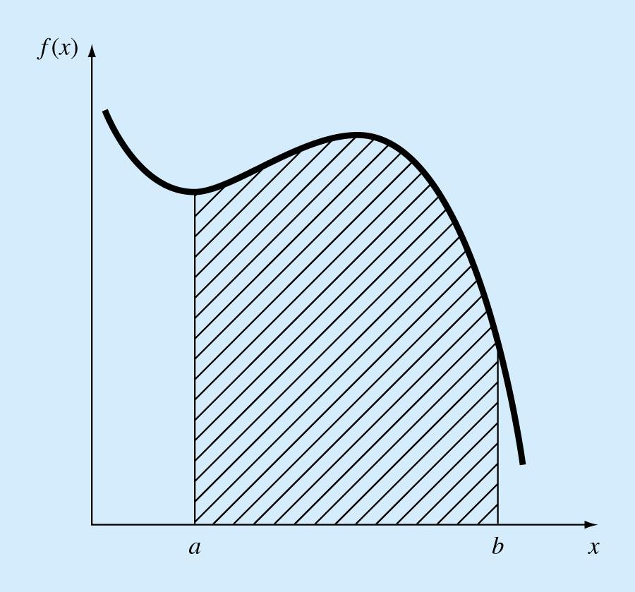
119

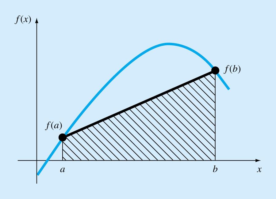
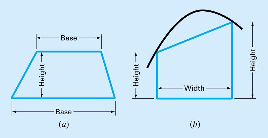
120

121

122 Example f(x) = exp(-x 2 ) Use left Riemann sum Integrate from 0 to 2 Exact value is N Sum

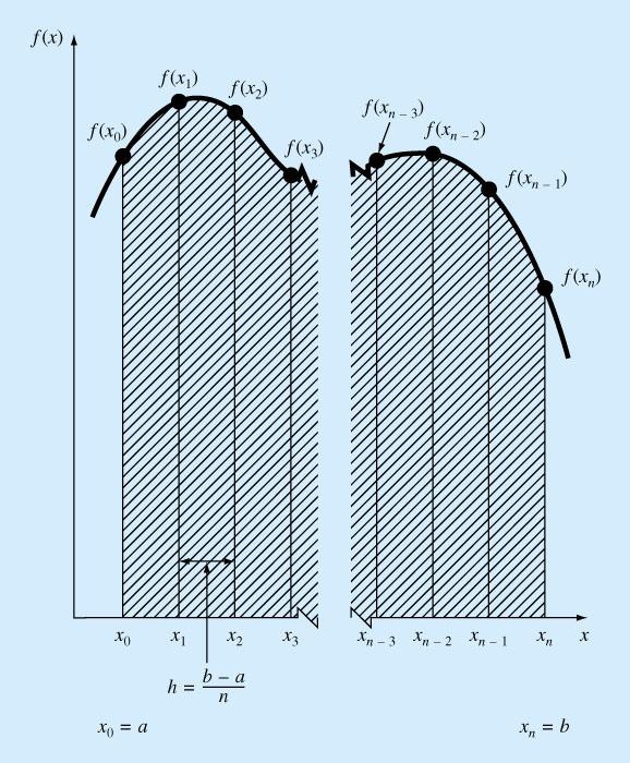
123 Trapezoidal Rule Simple Riemann sum approximates the function over each interval by a constant function We can use linear, quadratic, etc. instead for more accuracy Using a linear approximation over each interval results in the trapezoidal rule

124 Linear and Quadratic Approximations

125 Linear Approximations over Short Intervals

126 Closed and Open Rules

127 Trapezoidal Rule for an Interval b a ( a, f( a)) ( b, f( b)) f( b) f( a) f1( x) = f( a) + ( x a) b a f( b) f( a) f1( x) dx = f ( a) x + ( x a) 2( b a) f( b) f( a) 2 = f( a) b+ ( b a) f( a) a 2( b a) f( b) f( a) = f( a)( b a) + ( b a) 2 f( b) + f( a) = ( b a) 2 2 b a

128

129

130 Trapezoidal Rule for a Subdivided Interval Divide the interval [a, b] into n equal segments, each of width (b-a)/n Apply the trapezoidal rule to each segment Add up all the results This is much more accurate than the simple Riemann sum

131 h = ( b a)/ n x = a + ih i = 0,1, 2,, n f i i = f( x ) i 0.5 h( f + f ) h( f + f ) h( f + f ) h( f + f ) n 2 n 1 n 1 n n 1 0 i n i= 1 0 i n i= 1 2n = 0.5h f + 2 f + f = nh n 1 f + 2 f + f = 2n = n 1 f + 2 f + f 0 i n i 1 ( b a) = (width)(average he ight)

132

133

134

135 Example f(x) = exp(-x 2 ) Use trapezoidal rule Integrate from 0 to 2 Exact value is N Sum

136

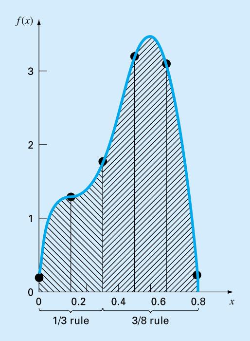
137 Simpson s Rules

138 Simpson s Rules Simpson s rules generalize the trapezoidal rule to use more than two points per interval, so we can use quadratic or cubic models instead of linear We will mainly cover the quadratic model, or Simpson s 1/3 rule

139 Quadratic Interpolation For a single interval, we will derive Simpson s 1/3 rule We will need to find the quadratic equation that goes through three points (x 1, f(x 1 )), (x 2, f(x 2 )), (x 3, f(x 3 )) We will then integrate the quadratic to obtain the estimate of the integral This also integrates cubics exactly

140 f = f( x ) f = f( x ) f = f( x ) h= x2 x1 = x1 x0 ( x x )( x x ) ( x x )( x x ) ( x x )( x x ) f( x) = f + f + f ( x x )( x x ) ( x x )( x x ) ( x x )( x x ) h f x x x x x f x x x x f x x x x f x 2 1 2h f( x) dx= ( )( 2 ) ( 2 ) 1 ( ) y h y h f y y h f + y y h f dy x h 0 h f0 + 4 f1+ f2 = ( f f 1+ f 2) = 2 h = width/average height ( ) = ( 1)( 2) 0 2( 0)( 2) 1+ ( 0)( 1) 2 2h 0 2h 0 2h y( y h) dy = y hy = h 2h = h h ( y h)( y 2 h) dy = y hy + 2h y = h 6h + 4h = h h 2 yy ( 0 2h h) dy = y + 2hy = h + 8h = h

141 Simpson s 1/3 Rule for a Subdivided Interval Divide the interval [a, b] into n equal segments, each of width (b-a)/n Apply the Simpson s 1/3 rule to each pair of segments Add up all the results This is more accurate than the trapezoidal rule

142 h f 4 f f f 4 f f f 4 f f f 4 f f 3 h f 0 4 f 1 2 f 2 4 f 3 2 f 4 2 f n 4 4 f n 3 2 f n 2 4 f n 1 f n 3 n 2 m is even n 4 n 3 n 2 n 2 n 1 n

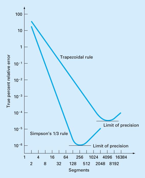
143 Example f(x) = exp(-x 2 ) Use Simpson s rule Integrate from 0 to 2 Exact value is N Sum

144 Simpson s 3/8 Rule Uses four points to fit a cubic polynomial Is not theoretically more accurate than the 1/3 rule, but can use an odd number of segments We can combine this with Simpson s 1/3 rule if the number of segments is odd With 15 intervals (16 points), this is 6 Simpson s 1/3 rule plus 1 of Simpson s 3/8 rule

145 3h = [ f ] f 1+ 3 f 2 + f 3 8 f + 3f + 3f + f = ( b a) 8 = (width)(average height)

146

147

148 Theoretical Errors of Newton-Cotes Methods Left and right Riemann integral formulas have errors of O(h). In the case of a linear function, y = c+dx for example, integrated over the interval [a, b], each approximating rectangle is missing a triangular portion whose base is h and whose height is dh, and there are n such triangles (h is the length of the interval divided by n), so the total error is ndh 2 /2 = d(b-a)h/2, which is proportional to h

149 Improving Left and Right Riemann Sums We can eliminate these triangles in two ways We can use a central Riemann sum that uses points in the middle of the intervals (open rule). This fits straight lines exactly We can use the trapezoidal rule, which also fits straight lines exactly Both these have O(h 2 ) errors

150 Error in Simpson s Rule The error in Simpson s 1/3 rule is is O(h 4 ) Compare this to left and right Riemann sums with errors at O(h) and the central Riemann sum and trapezoidal rule with errors at O(h 2 ) This means that in general Simpson s rule is more accurate at a given value of n It also gives information about changes of errors with n

151 Absolute Errors of Three Integration Methods f(x) = exp(-x 2 ), Integrate from 0 to 2, Exact value is N R L Trap Simp

152 Is the function available? The Newton-Cotes rules we have been looking at need a vector of function values The programs seen previously do not explicitly call a function; rather use a provided grid of values These methods can also be used in the form where a function is called In the case that any value can be called, other methods are available

153

154 Fixed Interval vs. Functional Integration The Newton-Cotes methods we have been describing all begin with a set of equally spaced function values. Sometimes this is all that is available, but we may be able to do better with some variation in the x s.

155 Richardson Extrapolation Given two estimates of an integral with known error properties, it is possible to derive a third estimate that is more accurate We will illustrate this with the trapezoidal rule, though the idea applies to any integration method with an error estimate

156 b f ( x ) dx = I = I ( h ) + E ( h ) a For the subdivided interval trapezoidal rule b a Eh = Oh = h f ξ 12 I= Ih ( ) + Eh ( ) = Ih ( ) + Eh ( ) 2 2 ( ) ( ) ''( ) for some in [a, b] Eh ( ) h f''( ξ ) h Eh ( ) h f''( ) h = ξ2 2 h Eh ( ) ( ) Eh 2 2 h2 h Ih ( 1) + h Eh ( ) Eh ( ) Ih ( ) + Eh ( ) h1 / h Ih ( ) Ih ( ) Ih ( ) Ih ( ) I= Ih + Eh = Ih + Oh ( 2) ( 2) ( 2) which has error ( ) 2 2 h1 / h2 1 ξ

157 For the special case where h = h / 2 I= Ih ( ) + Eh ( ) = Ih ( ) Ih ( ) Ih ( ) h1 / h2 1 Ih ( 2) Ih ( 1) Ih ( 2) Ih ( 1) = Ih ( 2) + = Ih ( 2) = Ih ( 2) Ih ( 1) e x 2 dx = I(0.2) = (n=10) I(0.1) = (n=20) 4 1 I(0.1) I(0.2) = comparable to Simpson's rule with n = 20

158 Repeated Richardson Extrapolation With two separate O(h 2 ) estimates, we can combine them to make an O(h 4 ) estimate With two separate O(h 4 ) estimates, we can combine them to make an O(h 6 ) estimate, etc. The weights will be different for these repeated extrapolations

159 I, I, I I = I I / I = I I / I = I I / 20 /10 40 / / = I I + I

160 Errors for Richardson Extrapolation from Trapezoidal Rule Estimates n T R1 R

161 Romberg Integration Let I j,k represent an array of estimates of integrals k = 1 represents trapezoid rules O(h 2 ) k = 2 represents Richardson extrapolation from pairs of trapezoid rules O(h 4 ) k = 3 represents Richardson extrapolation from pairs of the previous step at O(h 6 ), etc.

162 If we double the number of points (halve the interval) at each step, then we only need to evaluate the function at the new points For example, if the first step uses four intervals, it would involve evaluation at five points, the second one would use eight intervals, evaluated at nine points, only four of which are new I 4 k 1 I I = j+ 1, k 1 jk, 1 jk, k 1 4 1

163

164 Romberg starting with 2 intervals = 3 points True value is , requires 17 function evaluations to achieve 7-digit accuracy. Simpson s rule requires 36 function evaluations, and the trapezoid rule requires 775!

165 Exact Integration The trapezoidal rule integrates a linear function exactly using two points Simpson s 1/3 rule integrates a quadratic (and cubics also) exactly using three points It is possible to take n+1 evenly spaced points and choose the weights so that the rule integrates polynomials for degree n exactly (e.g., Simpson s 3/8 rule)

166 Gaussian Integration Consider a function f() on a closed interval [a, b] We assume f() is continuous We wish to choose n points in [a, b] and weights, so that the weighted sum of the function values at the n points is optimal Can be chosen to integrate polynomials of degree 2n-1 exactly

167 Two interior points can integrate more exactly than two end points

168 Two integrals that should be integrated exactly by the trapezoid rule Method of undetermined coefficients

169 b f( a) + f( b) f ( x) dx ( b a) =c0f(a)+c1f(b) Trapezoid Rule a 2 f ( x) = 1 and f ( x) = x should be integrated exactly 0 1 b a 1dx = c 1+ c b- a = h = c + c b b a 0 1 xdx = c a + c b 0 1 a = ca 0 + cb 1 = ca 0 + ( b a c0) b = 2 ( ) b a b ab c0 a b = c 2 ( a b) 2 c0( a b) b a = = c 2 0 1

170 0 2 1 b a b a f ( x) dx =c f +c f +c f dx = b a = c + c + c b b a xdx = = c0a + c1( a + b)/2+ c2b a 2 b b a x dx c a c a b c b a 3 c = c = ( b a)/ = = 0 + 1( + ) /4+ 2 c = 4( b a) / 6 Simpson's rule

171 Gauss-Legendre Find n points in [-1, 1] and n weights so that the sum of the weighted function values at the chosen points integrates as high a degree polynomial as possible n points and n weights means 2n coefficients, which is the number in polynomials of degree 2n 1 We find the two-point Gauss-Legendre points and weights for [-1, 1]; other intervals follow by substitution

172 c x x f( x) dx c f( x ) + c f( x ) 1dx = 2= c + c xdx = 0 = c x + c x x dx = = c x + c x x dx = 0 = c x + c x = c = 1 = =

173 Gaussian Quadrature Gauss Legendre is highly accurate with a small number of points Suitable for continuous functions on closed intervals Gaussian quadrature also comes in other forms: Laguerre, Hermite, Chebychev, etc. for functions with infinite limits of integration, or which are not finite in the interval

174 With n points, Gauss-Laguerre integrates functions exactly that are multiples of w(x) = e -x by polynomials of degree 2n-1 exactly. w(x) is called the weight function. The weight function for Gauss-Legendre is w(x) = 1.

175 2 2 1/2 wx ( ) = (1 x) Chebyshev, first kind 2 1/2 wx ( ) = (1 x) Chebyshev, second kind x wx ( ) = e Laguerre α x wx ( ) = xe Generalized Laguerre x wx ( ) = e Hermite

176

177

178

179 Numerical Differentiation Previously we learned the forward, backward, and centered difference methods for numerical differentiation These use the first-order Taylor-series expansion These can be made more accurate by using higher order Taylor series expansions

180 First-Order Forward Difference f ''( x ) f x+ h = f x + f x h+ h + O h 2 f ''( x ) f x h f x h f x h O h 2 f( x+ h) f( x) f ''( x ) f x h Oh h 2 f( x+ h) f( x) f'( x) = + Oh ( ) h ( ) ( ) '( ) ( ) '( ) = ( + ) ( ) + ( ) 0 2 '( ) = + ( )

181 First-Order Second Forward Difference x x = h j+ 1 j x, x,, x, x, x, 0 1 i i+ 1 i+ 2 f ''( xi ) 2 3 f( x) = f( xi) + f '( xi) h+ h + O( h ) 2 f ''( xi ) 2 f( xi+ 2) 2 f( xi+ 1) + f( xi) = f( xi) + f '( xi)2h+ 4h 2 f ''( xi ) 2 2 f( xi) + f '( xi) h+ h + f( xi) + O( h ''( i ) ( ) = f x h + Oh f( xi+ 2) 2 f( xi+ 1) + f( xi) f''( xi ) = + Oh ( ) 2 h 3 )

182 Second-Order Forward Difference f( xi+ 1) f( xi) f ''( xi) 2 f'( xi ) = h+ Oh ( ) h 2 f( xi+ 2) 2 f( xi+ 1) + f( xi) f''( xi ) = + Oh ( ) 2 h f( x ) f( x ) f( x ) 2 f( x ) + f( x ) f x Oh h 2h f( xi+ 2) + 4 f( xi+ 1) 3 f( xi) 2 f'( x) = + Oh ( ) 2h f( x+ h) f( x) + Oh ( ) h i+ 1 i i+ 2 i+ 1 i 2 '( i ) = + ( )

183 f( x) = e x 2 x = 2 h =.2 f (2.0) = f (2.2) = f (2.4) = f(2.2) f(2.0) = f(2.4) + 4 f(2.2) 3 f(2.0) = f '( x) = 2xe x f '(2.0) =

184 Numerical error as a function of step size and method h E1 O(h) E2 O(h 2 )

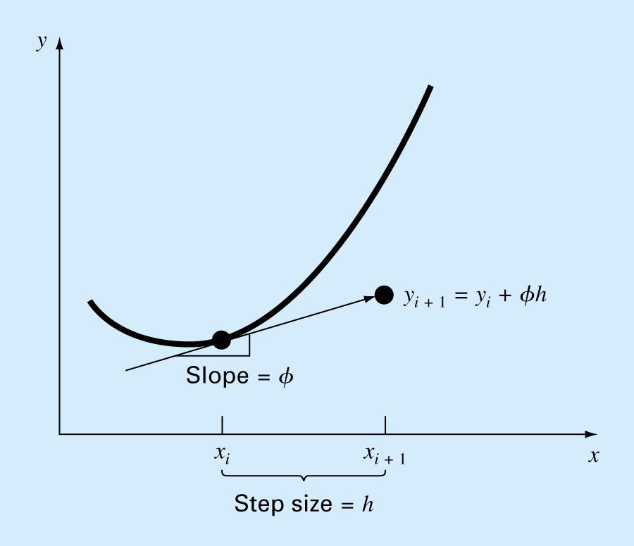
185 Factors affecting approximation accuracy First or second order method Forward or centered difference Step size All these affect the accuracy of the method

186 h Forward 1 O(h) Forward 2 O(h 2 ) Center 1 O(h 2 ) Center 2 O(h 4 ) E E E E E E E E E E E E E E E E E E E E-10

187 Richardson Extrapolation Just as with numerical integration, estimates with different errors can be combined to reduce the error Can be applied iteratively to further reduce the error as in Romberg integration

188 D= Dh ( ) + Eh ( ) k Eh ( ) = Oh ( ) D= Dh ( ) + Eh ( ) = Dh ( ) + Eh ( ) E( h) kh h Eh ( ) kh h k k = k k h Eh ( ) ( ) k 1 1 Eh k 2 h2 h Dh ( ) Eh ( ) Dh ( ) Eh ( ) k k h2 2 Eh ( ) 2 Dh ( ) Dh ( ) h 2 1 k k 1 / h2 1 D= Dh + Eh Dh + Dh ( ) Dh ( ) Oh 2 1 k + 2 ( 2) ( 2) ( 2) which has error ( ) k k h1 / h2 1

189 h h = 2 1 /2 / h = 2 k k k 1 2 Dh ( ) Dh ( ) 2 Dh ( ) Dh ( ) Dh ( 2) + = h k = 2 h k k k k 1 / h Dh ( ) Dh ( ) 4 Dh ( ) Dh ( ) Dh ( 2) + = h k k 1 / h2 1 3

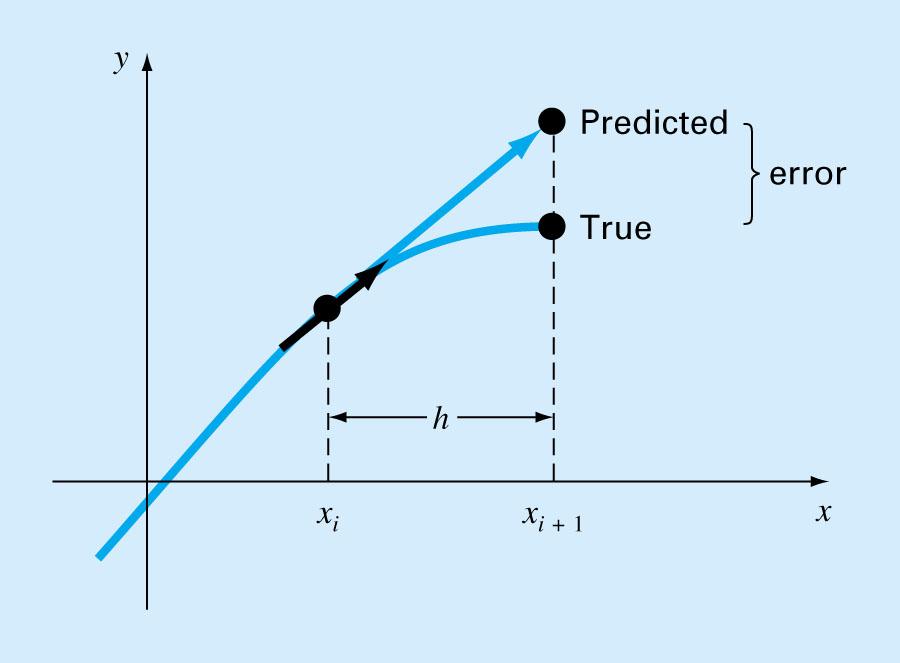
190 Ordinary Differential Equations ODE: solve for functions of one variable Possibly multiple equations and multiple functions, but usually one equation in one variable Functions of more than one variable can appear in partial differential equations (PDE s) Some ODE s can be solved analytically, but most cannot

191 Initial/Boundary Value Problem An initial value problem is an ODE in which the specifications that make the solution unique occur at a single value of the independent variable x or t A boundary value problem specifies the conditions at a number of different x or t values

192 Consider an ODE of the form dy = f( xy, ) with initial conditions dx We can trace out a solution starting at ( x, y ) y = y + φh i+ 1 where x x = h i+ 1 dy φ = dx i i 0 0

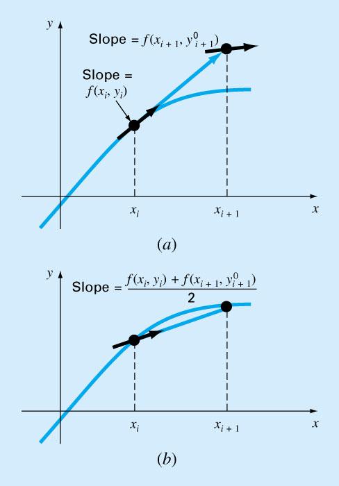
193

194

195 Runge-Kutta methods Euler s method is the simplest of these one-step methods Improved slope estimates can improve the result These methods are called in general Runge-Kutta or RK methods

196 dy = f( xy, ) dx y = y + φh i+ 1 i dy φ = = dx ( x, y ) Euler's method i i f( x, y ) i i

197 Errors in Euler s Method Errors are local to each step global or accumulated Errors are caused by truncation (when h is large) roundoff (when h is small and number of steps is large)

198 Euler s Method Is simple to implement Can be sufficiently accurate for many practical tasks if the step size is small enough No step size will result in a highly accurate result Higher order methods are needed

199 Improvements in Euler s Method We could use a higher order Taylor expansion at the current iterate to reduce truncation error This results in more analytical complexity due to the need for more derivatives Mostly, alternative methods are used to make the extrapolation more accurate Extrapolation is a hazardous business!

200 Heun s Method One problem with Euler s method is that it uses the derivative at the beginning of the interval to predict the change within the interval Heun s method uses a better estimate of the change, which is closer to the average derivative in the interval, rather than the initial derivative It is one of a class of predictor-corrector methods

201

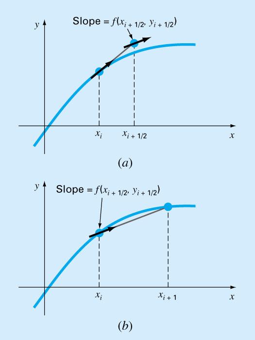
202 y = f( x, y ) i i i y y + f( x, y ) h Euler Step Predictor Equation 0 i+ 1 i i i y = f( x, y ) 0 i+ 1 i+ 1 i+ 1 y = i f( x, y ) + f( x, y ) 0 i i i+ 1 i f( xi, yi) + f( xi 1, yi 1) + + yi+ 1 = yi + h Corrector Equation 2 Can be iterated

203 a Integrate y = e y x = x = 0.8x from 0 to 4 with stepsize = 1 x = 0 then y = 2 Analytical y = ae + be 0.8x 0.5x y = 0.8ae 0.5be 0.8x 0.5x ( 0.8a ) ( ) ( ) 0 = y 4e + 0.5y = 0.8ae 0.5be 4e + 0.5ae + 0.5be a = + b= = + 4 / x 0.8x 0.5x 0.8x 0.8x 0.5x a e 0.8x 4 y = ( e e ) + 2e x 0.5x 0.5x

204 y = e y x = x = 0.8x from 0 to 4 with stepsize = 1 x = 0 then y = 2 x = 0 y = 2 y = 4-1 = y1 = 2 + 3(1) = 5 (true value at x = 1 is ) ε = / = t e = 0.8 y 1=4 0.5(5) y = ( ) / 2 = y 1 1 t = 2 + (4.7011)(1) = ε = / = 0.082

205 y = e y x = x = 0.8x from 0 to 4 with stepsize = 1 x = 0 then y = 2 x = 0 y = 2 y = 4-1 = 3 y y = 2 + 3(1) = 5 (true value at x = 1 is ) = 2 + (4.7011)(1) = = 0.8 y 1=4e 0.5(6.7010) y = ( ) / 2 = y 2 1 t = 2 + (4.2758)(1) = ε = / = 0.013

206

207 This will not, in general converge upon iteration to the true value of y i+1 This is because we are at best estimating the actual slope of the secant by the average of the slopes at the two ends, and even were the slopes at the two ends exact, this is not an identity

208 Integrate between 0 and 4, with y = 1 at x = 0 dy dx = x + x x x = 0 y = 1 h= Euler's Method x = 0.5 y = 8.5 y = 1 + (8.5)(0.5) = Heun's Method y = 1.25 y = y = 1+ (4.875)(0.5) = No iteration needed (True value is 3.00)

209 Midpoint Method Euler s method approximates the slope of the secant between two points by the slope at the left end of the interval Heun s method approximates it by the average of the estimated slopes at the endpoints The midpoint method approximates it by the estimated slope at the average of the endpoints

210

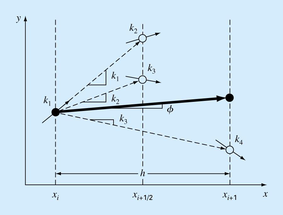
211 y 1/2 Integrate by midpoint method y = e y x= x= 0.8x from 0 to 4 with stepsize = 1 x= 0 then y = 2 x = 0 y = 2 y = 4-1= = 2 + 3(1/ 2) = 3.5 (true value at x= 1/ 2 is ) = 0.8/ 2 y 1/2 =4e 0.5(3.5) 1 t y = 2 + (4.2173)(1) = ε = / = / =

212 y = i f( x ) y y + f( x ) h Euler 0 i+ 1 i i y = f( x ) i+ 1 i+ 1 i f( xi) + f( xi+ 1) y i = 2 f( x ) + f( x ) = + 2 i i+ 1 yi+ 1 yi h f( x ) + f( x ) = 2 Trapezoid Rule i i+ 1 yi+ 1 yi h Heun

213 y = i f( x ) 0 + i+ 1 i i y y f( x ) h Euler = Riemann left y = f( x ) i+ 1/2 i+ 1/2 y = y + f( x ) h i+ 1 i i+ 1/2 Midpoint = Riemann midpoint y y = f( x ) h i+ 1 i i+ 1/2 i

214 Integrate between 0 and 4, with y = 1 at x = 0 dy = x + x x+ dx x = 0 y = 1 h= Euler's Method x = 0.5 y = 8.5 y = 1 + (8.5)(0.5) = Heun's Method y = 1.25 y = y = 1+ (4.875)(0.5) = Midpoint Method y = y = 1 + ( )(.5) = /2 1 (True value is 3.00)

215 Error Analysis Euler s method integrates exactly over an interval so long as the derivative at the beginning is the same as the slope of the secant line. This requires the derivative to be constant. y = f(x) = ax + b fulfills this requirement. The function must be linear. If f(x) is quadratic, then Heun s method and the midpoint method are exact

216 2 f x ax bx c ( ) f ( x ) f ( x ) = ( ax + bx + c) ( ax + bx + c) f( x ) f( x ) x x = + + = ax ( x) + bx ( x) [ ] = ( x x) ax ( + x) + b = ax ( + x) + b 1 0 f ( x1) + f ( x0) 2ax1+ b + 2ax0 + b = = ax ( 1+ x0) + b 2 2 f (( x + x )/2) = 2 a( x + x )/2 + b= a( x + x ) + b

217 Error Analysis If the function f(x) is approximated by a Taylor series, then Euler s method is exact on the first-order term, so the local error is O(h 2 ) Heun s method and the midpoint method are exact on the second-order approximation, so the local error is O(h 3 ) Since we are integrating O(h) intervals, the global error is O(h) for Euler and O(h 2 ) for Heun and the midpoint method

218 General Runge-Kutta Methods Achieve accuracy of higher order Taylor series expansions without having to compute additional terms explicitly Use the same general formulation as Euler s method, Heun s method, and the midpoint method in which the next point is the previous point plus the stepsize times an estimate of the slope.

219 y = f( xy, ) y i+ 1 i i i 1 φx = yy+ hh (,, ) φ= ak + ak + + ak k f( x, y ) i i k = f( x + ph, y + q kh) 2 i 1 i 11 1 k = f( x + ph, y + q kh+ q kh) 3 i 2 i n k = f( x + p h, y + q kh+ + q k h) n i n 1 i n 11 1 n 1n 1 n 1 n = 1 Euler's method n = 2 Heun/Midpoint method p = = 1 q = 1 a = 1/ 2 a = 1/ p = 1/ 2 q = 1/ 2 a = 0 a = n

220 Second-Order Runge-Kutta y = f( xy, ) yi+ φx 1 = yiy+ hh ( i, i, ) φ= ak 1 1+ ak 2 2 k1 = f( xi, yi) k2 = f( xi + ph 1, yi + q11kh 1 ) yi+ 1= yi + ( ak 1 1+ ak 2 2) h 1 d yi+ 1 yi + f( xi, yi) h+ f( xi, yi) h 2 dx d f( xy, ) f( xy, ) dy f( xy, ) = + dx x y dx y y + f( x, y ) h+ i+ 1 i i i 1 2 f + x 2 f dy h y dx 2

221 y = y + ( ak + ak ) h i+ 1 i f f dy yi+ 1 yi + f( xi, yi) h+ + h 2 x y dx k = f( x, y ) 1 i i f k2 = f( xi + ph 1, yi + q11kh 1 ) f( xi, yi) + ph 1 + q11kh 1 x 2 f 2 yi+ 1 = yi + ahf 1 ( xi, yi) + ahf 2 ( xi, yi) + ah 2 p1 + ahq 2 11 f( xi, yi) x = y+ af( x, y) + a i 1 i i 2 2 [ f( x, y )] h+ a p + a q f( x, y ) h 1= a+ a = 2a p = 2aq a = 1 a p = q = 1/2a f x f y 2 i i i i f y f y

222 y = y + ( ak + ak ) h i+ 1 i k 1 = f( x, y ) i k = f( x + ph, y + q kh) 2 i 1 i 11 1 a = 1 a p = q = 1/2a a = 1/2 a = 1/2 p = q = y = y + h( f( x, y ) + f( x + h, y + f( x, y ) h))/2 i+ 1 i i i i i i i Heun's Method i

223 y = y + ( ak + ak ) h i+ 1 i k 1 = f( x, y ) i i k = f( x + ph, y + q kh) 2 i 1 i 11 1 a = 1 a p = q = 1/2a a = 1 a = 0 p = q = 1/ y = y + hf( x + h/2, y + f( x, y ) h/2) i+ 1 i i i i i Midpoint Method

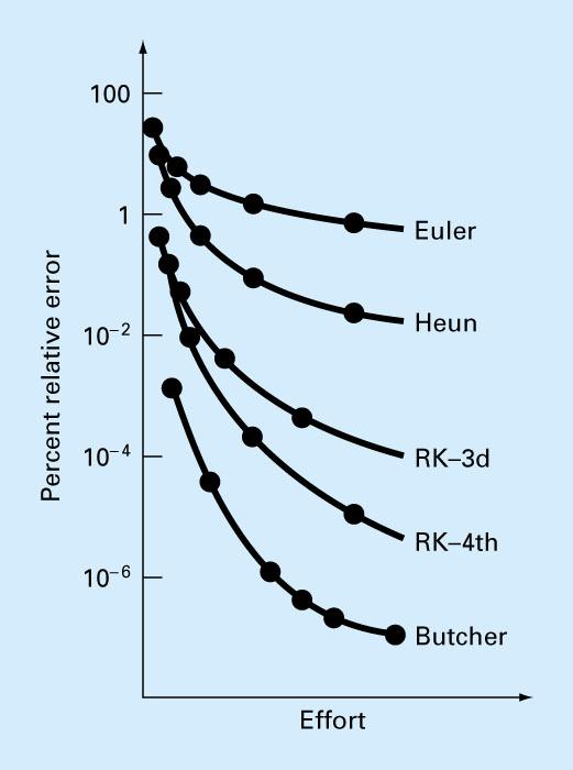
224 y = y + ( ak + ak ) h i+ 1 i k 1 = f( x, y ) i i k = f( x + ph, y + q kh) 2 i 1 i 11 1 a = 1 a p = q = 1/2a a = 2/3 a = 1/3 p = q = 3/ y = y + h( f( x, y ) + 2 f( x + 3 h/4, y + 3 f( x, y ) h/4))/3 i+ 1 i i i i i i i Ralston's Method

225 Higher-Order Methods Euler s method is RK order 1 and has global error O(h) Second-order RK methods (Heun, Midpoint, Ralston) have global error O(h 2 ) Third-order RK methods have global error O(h 3 ) Fourth-order RK methods have global error O(h 4 )

226 Derivation of RK Methods Second-order RK methods have four constants, and three equations from comparing the Taylor series expansion to the iteration. There is one undetermined constant Third-order methods have six equations with eight undetermined constants, so two are arbitrary.

227 y Third-Order Runge-Kutta y = f( xy, ) φx = yy+ hh (,, ) i+ 1 i i i φ= ak + ak + ak k 1 = f( x, y ) i i k = f( x + ph, y + q kh) 2 i 1 i 11 1 k = f( x + ph, y + q kh+ q kh) 3 i 2 i y = y + ( ak + ak + ak ) h i+ 1 i d 2 1 d yi+ 1 yi + f( xi, yi) h+ f( xi, yi) h + f( x, 2 i 2 dx 6 dx d f( xy, ) f( xy, ) dy f( xy, ) = + dx x y dx y ) h f( xy, ) f( xy, ) dy f( xy, ) dy f( xy, ) dy f( xy, ) = x x x y dx y dx y dx i 3

228 k 1 Common Third-Order Method = f( x, y ) i k = f( x + h/2, y + kh/2) 2 i i 1 k = f( x + h, y k h+ 2 k h) 3 i i 1 2 y = y + ( k + 4 k + k ) h/6 i+ 1 i i Reduces to Simpson's Rule

229 k 1 Standard Fourth-Order Method = f( x, y ) i k = f( x + h/2, y + kh/2) 2 i i 1 k = f( x+ h/2, y+ kh/2) 3 i i 2 k = f( x+ h, y+ kh) 4 i i 3 i y = y + ( k + 2k + 2 k + k ) h/6 i+ 1 i Reduces to Simpson's Rule

230

231 Comparing RK Methods Accuracy depends on the step size and the order Computational effort is usually measured in function evaluations Up to order 4, an order-m RK method requires m(b-a)/h function evaluations Butcher s order 5 method requires 6(b-a)/h

232

233 Systems of ODE s We track multiple responses y 1, y 2,, y n, each of which depends on a single variable x and on possibly all of the other responses We also need n initial conditions at x = x 0

234 dy dx dy dx 1 2 = = f( xy,, y,, y) f( xy,, y,, y) dyn = fn( xy, 1, y2,, yn) dx Euler's Method y = y + f( xy,, y,, y ) h ( i+ 1) () i () i () i () i j j j 1 2 n n n

235 dy dy = 0.5 y = 4 0.3y 0.1y dx dx Integrate x= 0 to x= with initial values y = 4y = 6, h= x y 1 y 2 y 1 y

236 RK Methods for ODE Systems We describe the common order 4 method. First determine slopes at initial value for all variables, this gives a set of n k 1 values. Then use these to estimate a set of functional values at the midpoint and slopes Use these to get improved midpoint values and slopes Use these to get estimate of value and slope at end Combine for final projection

237 dy dy = 0.5 y = 4 0.3y 0.1y dx dx Integrate x= 0 to x= with initial values y = 4y = 6, h= 0.5 k = f( x, y ) i 2 i i 1 3 i i 2 4 i i k = f( x + h/2, y + kh/2) k = f( x+ h/2, y+ kh/2) k = f( x+ h, y+ kh) i y = y + ( k + 2k + 2 k + k ) h/6 i+ 1 i

238 dy dy = 0.5 y = 4 0.3y 0.1 y dx dx x= 0, 2 y = 4y = 6, h= 0.5 k k k k ,1 1 1,2 2 2, , = f (0, 4,6) = 2 = f (0, 4, 6) = 4 0.3(6) 0.1(4) = 1.8 = f (0.25, 4 + ( 2)(0.5) / 2,6 + (1.8)(0.5) / 2) = f (0.25,3.5, 6.45) = 1.75 = f (0.25,3.5, 6.45) =

239 dy dy = 0.5 y = 4 0.3y 0.1 y dx dx x= 0, 2 y = 4y = 6, h= k = 2 k = 1.8 k = 1.75 k = k k k k 1,1 1,2 2,1 2,2 = f (0.25, 4 + ( 1.75)(0.5) / 2, 6 + (1.715)(0.5) / 2) 3,1 1 = f (0.25,3.5625, ) = = f 1 3,2 2 4, ,2 2 (0.25,3.5625, ) = = f (0.5, 4 + ( )(0.5), 6 + ( )(0.5)) = f (0.5, , ) = = f (0.5, , ) =

240 y y 1 2 dy dy = 0.5 y = 4 0.3y 0.1 y dx dx x= 0, 2 y = 4y = 6, h= k = 2 k = 1.8 k = 1.75 k = k k 1,1 1,2 2,1 2,2 = k = ,1 3,2 = k = ,1 4,2 (0.5) = 4 + ( 2 + 2( 1.75) + 2( ) + ( ))(0.5) / 6 = (0.5) = 6 + ( (1.715) + 2( ) )(0.5) / 6 =

241 Adaptive RK Methods A fixed step size may be overkill for some regions of a function and may be too large to be accurate for others Adaptive methods use different step sizes for different regions of the function Several methods for accomplishing this Use different step sizes but same order Use different orders

242

243 Adaptive RK or Step-Halving Predict over step with order 4 RK, obtain prediction y 1 Predict with two steps of half step size to obtain prediction y 2 Difference Δ = y 2 y 1 is an estimate of the error that can be used to control step size adjustment y 2* = y 2 + Δ/15 is fifth order accurate

244 0.8x y 4e 0.5y x = 0 to 2, h = 2 y(0) = 2 True value at 2 is Full step prediction k = f( x, y ) = f(0,2) = 3 1 = i i k = f( x + h/ 2, y + kh/ 2) = f(1,5) = i i 1 k = f( x+ h/ 2, y+ kh/ 2) = f(1, )= i i 2 k4 = f( xi + hy, i + k 3 h) = f(2, )= y = y + ( k + 2k + 2 k + k ) h/ 6 = i+ 1 i

245 y y 0.8x y = 4e 0.5y x = 0 to 2, h = 2 y(0) = 2 True value at 2 is Full step prediction is Half-step predictions are i+ 1 i+ 2 E E y E a t * t = 2 + (3 + 2( ) )1/ 6 = = ( ( ) )1/ 6 = = ( ) /15 = = = = ( ) = = =

246 Fehlberg/Cash-Karp RK Instead of using two different step sizes, we can use two different orders This may use too many function evaluations unless the two orders are coordinated Fehlberg RK uses a fifth order method using the same function evaluations as a fourth order method Coefficients due to Cash and Karp

247 (4) yi+ 1 = yi + k1+ k3+ k4 + k6 h (5) yi+ 1 = yi + k1+ k3+ k4 + k5 + k6 h k = f( x, y ) 1 i i 1 1 k2 = f( xi + h, yi + kh 1 ) k3 = f( xi + h, yi + kh 1 + kh 2 ) k4 = f( xi + hy, i + kh 1 kh 2 + kh 3 ) k5 = f( xi + h, yi kh 1 + kh 2 kh 3 + kh 4 ) k6 = f( xi + h, yi + kh 1 + kh 2 + kh 3 + kh 4 + kh 5 )

248 Values needed for RK Fehlberg for the example. x y f(x,y) k k k k k k

249 y (4) i = h = (5) yi+ 1 = yi h = E a = =

250 Step Size Control First we specify desired accuracy Relative error can be a problem if the function is near 0 Absolute error takes no account of the scale of the function One method is to let the desired accuracy depend on a multiple of both the function and its derivative

251 = ε y y new scale = y scale dy yscale = y + h dx h new = h present new present α α =.2 when the step size is increased α =.25 when the step size is decreased This is one scheme of many for adaptive step size

252 Example: 2 dy ( x 2) + 0.6y = 10exp dx 2(0.075) y(0) = 0.5 General Solution y = 0.5exp( 0.6 x) 2

253