The Optimal Location for the Salton Sea Pipelines

Transcription

1 University of Redlands Redlands MS GIS Program Major Individual Projects Geographic Information Systems 2016 The Optimal Location for the Salton Sea Pipelines Mohammed Saleh Alzaaq University of Redlands Follow this and additional works at: Part of the Geographic Information Sciences Commons Recommended Citation Alzaaq, M. S. (2016). The Optimal Location for the Salton Sea Pipelines (Master's thesis, University of Redlands). Retrieved from This Thesis is brought to you for free and open access by the Geographic Information Systems at Redlands. It has been accepted for inclusion in MS GIS Program Major Individual Projects by an authorized administrator of Redlands. For more information, please contact rebecca_clayton@redlands.edu, paige_mann@redlands.edu.

2 University of Redlands The Optimal Location for the Salton Sea Pipelines A Major Individual Project submitted in partial satisfaction of the requirements for the degree of Master of Science in Geographic Information Systems by Mohammed Saleh Alzaaq Ruijin Ma, Ph.D., Committee Chair Douglas Flewelling, Ph.D. August 2016

3 The Optimal Location for the Salton Sea Pipelines Copyright 2016 by Mohammed Saleh Alzaaq

4

5

6 Acknowledgements First, I would like to thank my family and my parents for supporting me through my education and my life. Without them, I would not be where I want to be. I also would like to thank the MS GIS faculty members for guiding me throughout this program. A special thanks to Dr. Ruijin Ma for spending the time to advise and help me with this project. Lastly, I would like to thank my Cohort 25.5 and Cohort 25 for supporting and helping me throughout this master s program. I spent these days with the best supportive group of people. Again, thank you so much. v

7

8 Abstract The Optimal Location for the Salton Sea Pipelines by Mohammed Saleh Alzaaq The Salton Sea, in southern California, is the largest lake in California with an area of 370 square miles. It has environmental issues such as salinity and drought. Dr. Timothy Krantz, the client of this project, proposed a solution to reduce the environmental impacts. The solution was to connect the Salton Sea to the Gulf of California using pipelines. As a result, the project s goal was to determine the optimal location for the pipelines to link these bodies of water considering multiple criteria. A least-cost path analysis was used to determine the best pipeline routes. Also, a weighted overlay analysis was used to discover suitable sites for solar farms adjacent to the pipelines. A paper map that locates the pipeline routes and solar sites was delivered to the client. Additionally, GIS tools, which were developed throughout the project s process, were submitted for future work on this project. vii

9

10 Table of Contents Chapter 1 Introduction Client Problem Statement Proposed Solution Goals and Objectives Scope Methods Audience Overview of the Rest of this Report... 4 Chapter 2 Background and Literature Review Least-Cost Path Approach Suitability Analysis Summary... 6 Chapter 3 Systems Analysis and Design Problem Statement Requirements Analysis Functional Requirements Non-Functional Requirements System Design Project Plan Summary Chapter 4 Database Design Conceptual Data Model Logical Data Model Data Sources Data Collection Methods Data Scrubbing and Loading Summary Chapter 5 Implementation Factors Analyzed for Pipelines Road Factor Slope Factor Cities Factor Rivers Factor Land Cover Factor Protected Land Factor Least-Cost Path Analysis Preparing Datasets for Solar Sites Analysis Weighted Overlay Analysis for Solar Sites Summary Chapter 6 Results and Analysis ix

11 6.1 Pipelines Map and Tool Solar Sites Maps and Tools Discussion Summary Chapter 7 Conclusions and Future Work Project Conclusion Future Work Works Cited Appendix A. Workflow for Pipelins Factors Appendix B. Workflow for Solar Sites Factors x

12 Table of Figures Figure 1-1: The Study Area for the Pipeline Routes... 2 Figure 3-1: System Design... 9 Figure 4-1: Conceptual Data Model Figure 4-2: The DEM Data Collection for Different Regions of the Study Area Figure 4-3: The Completed DEM Data for the Study Area Figure 4-4: The Original Dataset from the USGS and the Completed Land Cover Dataset Figure 4-5: The Received Roads Data and the Final Roads Datasets Figure 5-1: Distance Values for the Roads Datasets Using the Euclidean Distance Tool Figure 5-2: Roads Values after Changing Using the Raster Calculator Tool Figure 5-3: The Cost Surface for the Roads Dataset Figure 5-4: Slope Factor Values Figure 5-5: Slope and Roads Cost Surface Figure 5-6: Cost Surface for Cities Figure 5-7: Workflow for Cities Cost Surface Figure 5-8: Buffer Map for the River in the Study Area Figure 5-9: The River Cost Surface Figure 5-10: Workflow for Rivers Cost Surface Figure 5-11: Raster Calculator for the Land Cover Types Figure 5-12: The Cost Surface for the Land Cover Dataset Figure 5-13: The Equation to Convert the Protected Land Dataset Figure 5-14: The Cost Surface for the Protected Land Figure 5-15: The Workflow for the Main Cost Surface Figure 5-16: Thr Workflow for the Least-Cost Path Method Figure 5-17: Pipelines Elevation Profile Figure 5-18: Influence and Values for the Slope Factor Figure 5-19: Influence and Values for the Solar Radiation Factor Figure 5-20: Influence and Values for the Distance from the Pipelines Factor Figure 6-1: The Final Analysis Tool for Pipelines Figure 6-2: Proposed Optimal Location for Pipelines Figure 6-3: The Solar Site Tool for 60 and 20-Meter Elevation Areas Figure 6-4: Suitability Surface for Solar Sites at the 60-Meter Elevation Area Figure 6-5: Suitability Surface for Solar Sites at the 20-Meter Elevation Area Figure 6-6: Pipelines and Solar Sites as the Final Map for this Project Figure 6-7: The Relations between the Cost and the Distance to a Road Figure 6-8: Cost Surface for the Pipeline Routes Close to the Roads Figure 6-9: The High-Cost Surface Values for the Protected Area Figure 6-10: The Cost Surface without the Land Cover Factor Figure A-1: The Road Factor Workflow Figure A-2: Slope Factor Workflow with Road Factor Figure A-3: The Workflow for the Land Cover Figure A-4: The Workflow for the Protected Land Factor xi

13 Figure B-1: Steps for Preparing Datasets for Solar Sites Analysis Figure B-2: The Three Analyzed Factors for the Solar Sites xii

14 List of Tables Table 3-1 Project Plan Table 4-1 Logical Data Model Table 4-2 Data Source and Type Table 5-1 Land Cover Types and Their Values Table 5-2 The Reclassification for the Slope Factor Table 5-3 The Reclassification for the Solar Radiation Factor Table 5-4 The Reclassification for the Distance to Pipelines Factor xiii

15

16 List of Acronyms and Definitions CEC CSP DEM GIS PV SSA SSDP USGS Commission for Environmental Cooperation Concentrated Solar Power Digital Elevation Model Geographic Information System Photovoltaic Solar Power Salton Sea Authority Salton Sea Database Program United States Geological Survey xv

17

18 Chapter 1 Introduction The importance of steady water availability appears when drinkable water resource represents only three percent of all the water on the planet. The need for planning, developing, distributing, and managing a water resource is essential to maintain sustainable life in any general area. However, the Salton Sea, in southern California, has a high level of salinity that causes several environmental concerns. These concerns affect the vegetation, animal species, and the habitats within the area. Undertaking such a project should minimize the environmental impact of water use on the natural environment. This project intended to solve this issue by developing maps and tool using Geographic Information System (GIS) technology to find suitable paths for pipelines between the Salton Sea and the Gulf of California. This project would be an opportunity to learn and apply its findings in the future. As a geographer, protecting nature from danger is the primary goal. This project was an opportunity to use GIS technology to help inhabitants in the Salton Sea and the Salton Sea Authority (SSA) to make decisions regarding the Salton Sea s salinity. Water resources are a natural issue, especially in countries where most areas are desert, such as the Middle East. Pipelines and canals are usually proposed to solve these issues. For instance, there was a proposed project in Saudi Arabia to build a canal from the Red Sea to the Arabian Gulf. However, this plan was not approved because of evaporation and the long distance. This project was an excellent opportunity to be observed by the Middle East countries by providing a new water resource using the experience from this project. This chapter is divided into five sections. The client s information is reviewed in section 1.1, followed by the problem statement in section 1.2. Section 1.3 discusses the project s proposed solution and contains goals, scope, and methods used. Audiences are reviewed in Section 1.4, followed by an overview of the rest of this report in the last section. 1.1 Client The client was Dr. Timothy Krantz, a professor of environment studies at the University of Redlands. He is the director of the Salton Sea Database Program (SSDP), where the data of Salton Sea are managed, stored, and analyzed to support research and develop tools to help people who are interested in maintaining the Salton Sea. Dr. Krantz has been working on renewable-energy technologies, sustainable green buildings, and environmental impact assessments over the past several years. In particular, he focused on the Salton Sea and spent a lot of time researching and studying the targeted area. He also developed a regional geographic database for the Salton Sea area. He helped define the scope of this project and provided some of the data needed. 1

19 1.2 Problem Statement The suitability of drinkable water, irrigation water, and wildlife water depends on the salt concentration in the potable water. The problem with the Salton Sea is its higher level of salinity than most of the water resources surrounding the study area. According to Bail (2015), the Pacific Ocean s salinity is around 35 grams per liter, while the Salton Sea s salinity is about 54 grams per liter. Because of the high evaporation in the Salton Sea area and the lack of fresh water access to the sea, the concentration of the salt increases in the sea approximately 1% every year. To solve this problem, the client figured out a solution by connecting the Salton Sea to other water resource using pipelines. The major problem addressed in this project was identifying the suitable path for the pipelines in the study area (Figure 1-1). Agriculture, vegetation, rivers, and the habitats within the area must be considered when the pipelines are designed to reduce the negative impacts. To prevent future ecological and demographic changes and other harmful effects, better ideas of spatial solutions were defined in this project that were shareable and persuasive for decision makers. Figure 1-1: The Study Area for the Pipeline Routes. 2

20 1.3 Proposed Solution Because of the salty water, the Salton Sea should link to another water resource that has less salinity to solve this problem. Water pipelines have been proposed for transferring and pumping water into two bodies of water in the world. For example, the largest water pipeline project in China was used to transport water approximately 2,700 miles (Kuo, 2014). This project explored a suitable route for pipelines between the Salton Sea and the Gulf of California using ArcGIS technologies. Additionally, the project discovered solar sites around the pipelines. This project used least-cost path and weighted overlay analyses considering various human and natural factors. Salton Sea pipelines were proposed to carry surface water with a high level of salinity from the Salton Sea in southern California to the Gulf of California in Mexico. Also, the pipelines will transfer surface water with less salinity from the Gulf of California to the Salton Sea. Pipelines were chosen because they have less impact on the environment and reduce the chance of evaporation, which can occur in an open water transfer such as a canal. Another benefit of pipelines is that they transfer water quickly and efficiently by using pumps and the natural force of gravity. Pipelines also keep water clean, which means less pollution. They help control water flow in case of earthquakes by using controlled gates inside the pipelines. With all these advantages, they are the best solution for transporting water Goals and Objectives There were two primary goals in this project. The first goal was to produce a map that showed the best path for inflow and outflow pipelines between the Salton Sea and the Gulf of California. This route was designed to consider the natural environment and human factors. The natural environment elements were elevation, slope, rivers, and land cover. The human factors were cities, streets, agriculture, and protected land. These factors affect the route of the pipeline, and ArcGIS was used to analyze these factors for optimal ways. The second goal was to identify appropriate sites for alternative energy adjacent to the pipelines. These sites were completed to support the pipeline with energy for pumping water in the high-elevation areas. Also, these sites should be in suitable locations where there are little human activity, high values of wind, sun lights, and far away from cities to help solar energy fields operate efficiently Scope The goal of this project was to identify an appropriate route for pipelines and to locate solar sites beside the pipelines using GIS technology. There were many features to consider in the study area. The first element was the human factors including cities, roads, agriculture, and protected land. The second element was the natural factors: land cover, rivers, and slope. The start and end points of the pipelines were given by the client where the start point at the Salton Sea and the end point at the Gulf of California. These pipelines must follow the most suitable path between the two bodies of water because the water will travel on the ground surface. By using the power that comes from the solar 3

21 energy stations that were provided, the pipelines will be able to lift up water using pumps at the high-elevation sites in the study area. This project delivered a geodatabase of the factors datasets that were used to evaluate the pipeline routes. Also, a paper map that included the pipeline routes and solar sites was submitted to the client. Additionally, workflow tools of this project were explained and delivered to the client Methods This project required the ArcGIS application to organize, process, and analyze the data for the project. Powerful ArcMap analysis capabilities, such as the weighted overlay tool and least-cost path analysis, were used to create suitable pipeline routes and solar sites. The least-cost approach was used to develop the pipeline routes. These routes had spatial referencing and elevation profile that showed the highest and lowest pipeline elevation. The Digital Elevation Model (DEM) and major streets data for the study area were analyzed to have the slope data, the elevation values, and the streets network in raster format. Also, land cover and protected land datasets were evaluated depending on their importance according to the client needs. The weighted overlay approach was used to find the optimal location for solar energy in the study area. The solar radiation analysis extension tool in Spatial Analyst was used to determine the spatial variability of insolation such as elevation, orientation, shadows, air, and soil temperature (Esri, 2012). This tool was used to map and analyze the sun s effects for a specific area to discover appropriate sites for solar energy. 1.4 Audience This project will be published on the Internet via the Salton Sea Project website. The primary audience of this project was the Salton Sea Authority, which includes many government agencies. Riverside County, Imperial County, the Imperial Irrigation District, the Coachella Valley Water District, and the Cahuilla Indian Tribe are the main audience of the American side of this project. The Mexican government and geographic institutions could benefit from this project because it could be used to support them as a new water resource. 1.5 Overview of the Rest of this Report The historical background of the Salton Sea and the literature review are addressed in Chapter 2. Chapter 3 defines the system design with the analysis work and describes the project plan. The database design, the conceptual data model, the logical data models, and data information are provided in Chapter 4. Chapter 5 contains the workflow of this project and all the work that has been done to solve the project s problem. Chapter 6 identifies the solutions and the results from the work in Chapter 5. The last chapter includes a summary of the project and recommendations for potential future work. 4

22 Chapter 2 Background and Literature Review A literature review was significant helpful for specifying the methods that were to be used for this project. This project was intended to help the client discovers the optimal pipeline routes between the Salton Sea and the Gulf of California. Additionally, solar energy sites adjacent to the pipelines were requested to support the pipes with power. Many factors were considered in determining the pipeline routes and solar sites, such as elevation, roads, rivers, and land used. Two techniques were used to solve the project s problems. The first technique was least-cost path analysis. This method was used to find the optimal location for pipelines. The least-cost path analysis is addressed in section 2.1. Another technique, suitability analysis, was used to determine the best location for solar energy sites. This analysis is discussed in section 2.2, followed by a summary at the end of this chapter. 2.1 Least-Cost Path Approach The least-cost path is a common methodology that is used to connect two points using ArcGIS. To link these points, a cost surface should be created in a raster format. Each cell on the cost surface has a value that is affected by the factor values. The factors can be given relative values depending on their importance. After that, the cost surface can be calculated to determine the least-cost path between the two points. Some projects use this analysis for determining routes and utility pipelines. Chandio et al. (2012) described least-cost path analysis as an opportunity for planners and engineers to determine the most suitable land for routing a road. They used the least-cost path approach to find the best route for a road by integrating multiple criteria such as slope and land use. They also used this method to establish a road going uphill. Additionally, the Weighted Sum model was used to assign multiple criteria to a common scale. As a result, the cost surface was created, which determined the cost distance and the cost direction. Kelly (2014) developed a route for gas pipelines in western Turkey. Multiple factors were considered to reduce environmental impacts and risks to humans. Kelly (2014) stated that each factor was weighted according to its risk assessment. Therefore, these factors were combined using map algebra to create a cost surface. These factors were reclassified on a scale of 0 to 10, where 10 is unsuitable and 0 is suitable. A case study by Feldman et al. (1995) and an engineering report by Topal and Akin (2009) were used by Kelly to evaluate the specific value for each criterion. Feldman et al. (1990) stated that an actual pipeline project, called the Bechtel project, was used to calculate cost surface values. A geological survey was completed by Topal and Akin (2009) to provide landcost values for pipeline routes. Kelly (2014) developed four cost surfaces with different weighted overlay values. Mick and Teykl (2015), working with the City of Austin, Texas, developed a pipeline route using ArcGIS. The main goal for the project was to reduce the cost effect and environmental impact to transfer water efficiently. Mick and Teykl (2015) stated that they began by evaluating the main criteria for the route analysis. Afterward, they assigned each factor with a suitability value on a scale from 1 to 9, where 1 is the most 5

23 suitable and 9 is the least suitable. As a result, the suitability surface was created for the study area. They then applied an algorithm calculation for the optimal path, where they focused on minimizing unattractive areas and maximizing desirable areas. They used this method because the suitability surface was defined to force the pipeline path towards the suitable land. These projects are presented to show how the least-cost path approach was used to solve different project goals. Likewise, this approach was used in this project to discover the optimal routes for the Salton Sea pipelines. 2.2 Suitability Analysis There are different ways of identifying a suitable site for a solar farm. One common way used in various projects is weighted overlay analysis. This type of analysis was used in this project to discover sites that are optimal for solar power and would be adjacent to the pipeline routes. Likewise, some users apply this approach in order to identify desirable locations that meet their project s goals. For example, Orr (2011) developed a suitability tool using weighted overlay analysis. This tool is able to display solar sites and wind power applications depending on the user specifications. Also, the user could use several factors with different weighted values in order to meet the user s needs. Another project that used weighted overlay analysis was done by McKinney (2014) to discover suitable sites for solar farms in Watauga County, North Caroline. He described two types of solar power: photovoltaic (PV) and concentrated solar power (CSP). PV uses solar radiation that processes through a semiconductor in order to generate power. CSP uses sunlight to transfer heat into steam and then into power. McKinney (2014) used the Area Solar Radiation tool to develop raster surface with yearly average solar radiation and reclassify these values into 10 classes. He used slope, hillshade, aspect, and land cover as factors that affect the suitable site. These papers were used to clarify how weighted overlay analysis could be used and to determine the factors for this project s. 2.3 Summary The background and literature review discussed some methodologies used on this type of project. The first section described projects that used least-cost path analysis. Other projects that used suitability analysis were described in section 2.2. This chapter was intended to specify two methodologies that were used in this project. 6

24 Chapter 3 Systems Analysis and Design This chapter demonstrates the system analysis and design executed to achieve the objectives of this project. This chapter is divided into five parts: The problem statement is identified in the first part, and the requirements analysis is reviewed in the second part. The system design is explained and discussed in the third part. The project plan is defined in the fourth part, and the last part provides a summary of the chapter information. 3.1 Problem Statement The Salton Sea has a high level of salinity, and the client needed a solution for this environmental issue. A proposed solution by the client is to connect the Salton Sea to the Gulf of California by using ground pipelines. The problem addressed in this project is to find the most suitable path between these bodies of water. Many factors must be considered when this solution is designed in order to reduce the negative impact on habitats and the environment within the study area. 3.2 Requirements Analysis The requirements were discussed with the client to clarify the goal of this project. These requirements were divided into two parts: the functional and non-functional. The functional requirements were defined as being what the system should do or provide for the client, whereas the non-functional requirements were defined as being how the system could do the operations. This project had several functional and non-functional requirements Functional Requirements There were two types of functional requirements: those that addressed the entire project and those that addressed the model tool. The project functional requirements were that the project system shall: Display the result on a map. Perform the least cost path analysis to identify where to place the pipes. Analyze factors that were identified with the client. Create a polyline in a new feature class that represents the most suitable path for the pipelines. Develop a suitable surface that represent appropriate solar sites. The functional requirements of the pipeline tool were that the tool shall: Have datasets in the same projection and formats as raster datasets. Use only the data that were provided for this project: Start point End point Digital elevation modal Roads Rivers 7

25 Cities Land cover Protected land Generate the slope values from the DEM, to be used as one of the factors that affect the pipeline's path. Divide the road layer based on the type field as the following: Paved roads Unpaved roads No-Road Areas Convert the rivers, cities, and protected land datasets values to assign them as unsuitable lands. Transfer the land cover dataset values based on their type names. Add raster dataset values together using the Raster Calculator tool (The values were assigned according to the client s requests). Run the least-cost path analysis on the cost surface to have the final pipeline feature class. The functional requirements of the solar site tools were that the tools shall: Have datasets in the same projection and formats as raster datasets. Use only the data that were provided for this project: 60 and 20 meters elevation areas. Slope Area solar radiation Reclassify the data values based on the client s request. Apply the Weighted Overlay tool to have suitable sites for solar farms Non-functional Requirements The non-functional requirements were based on the technical considerations. The technology that was used to develop the system had to be compatible with the client s software. As a result, the system shall: Run on ArcGIS 10.2 for Desktop. Be built using ModelBuilder. Use the Esri platform for the dataset types. Be delivered in a file geodatabase that contained maps, datasets, and the project s workflow tools. 3.3 System Design The system design was created based on the project requirements that were discussed with the client. The system s components started with a file geodatabase that contained inputs, toolboxes, and an output. The input layers, provided by the client, were the factors that affected the pipeline routes. The data were added together to create a cost surface with start- and end- point layers. The Best Pipeline tool was customized using tools in ArcGIS toolbox to generate an optimal route for the pipelines in the study area. The Least-Cost Path tool was used to produce a line feature class as output that represented 8

26 the best path between the Salton Sea and the Gulf of California given the start and end points. The system design appears in Figure 3-1. Input Layer: Geoprocessing Land cover Roads Rivers Cities DEM Protected Land Least-Cost Path Pipeline Tool Weighted Overlay Solar Sites Tool Output Layer: Pipeline Routes Suitable Solar Sites Figure 3-1: System Design 3.4 Project Plan The project was broken down into four phases as it is shown in Table 3-1. The first phase was to identify the goal of the project and to create a plan for managing the data to be used. The client determined his objectives and provided some information such as the Salton Sea boundary and the study area river data. This phase took place during June- August The second phase, the developing process, involved the technical work including developing all the tools with ArcGIS using ModelBuilder. The Best Path tool was designed to draw the best route in the study area. In the third phase, the outcomes of the tools were discussed with the client to ensure his objectives would be met, and the project s map was designed so it could be seen by the client. The second and third phases took a place within September and October The last phase was deployment, final implementation of the project. The ultimate tool and map were completed and documented for submission to the client. This phase was scheduled for November - July 2016, before the deadline to present the project. 9

27 Table 3-1: Project Plan Task Title Start Month End Month Labor Hours Phase 1 Planning 1.1 Identify goals and objectives June July Collect and manage data August August 50 Phase 2 Development 2.1 Develop a tool for each factor. September September Add all tools to the Best Path September September 60 tool and run the tool 2.3 Discuss the analysis process September October 60 with the advisor Phase 3 Testing and Map Design 3.1 Test the outcomes October October Design the map October October Phase 4 Deployment 4.1 modify, complete, and review November November 60 the map with the client 4.4 Edit, document, and submit the project December July, Summary This chapter defined the system analysis and design and restated the problem this project is addressing. Also, this chapter described the functional and non-functional requirements. A graph for the system design and a table for the project plan were provided to illustrate further the project process. 10

28 Chapter 4 Database Design This chapter discusses the database design and the data that were used in this project. The conceptual data model is described in the first section of this chapter, followed by the logical data model. Sections 3.3 and 3.4 address the data source and the data collection methods. Data scrubbing and loading are explained in section 4.5, followed by a summary at the end of this chapter. 4.1 Conceptual Data Model A conceptual data model is one of the most common processes that explains the project plan and significant details about understanding the project. The conceptual data model (Figure 4-1) was developed for the project to identify the data requirements to solve the client s problem. The Salton Sea boundary and the Gulf of California border were needed because they were connected using pipelines. To connect these bodies of water with surface pipes, the human and physical qualities should be considered. Elevation, land cover, and rivers are the natural factors while cities and roads are the human factors that affect the suitable route in the study area. Isolation data and distances from pipelines were needed for alternative sites suitability for this project. All these factors were generated to define the suitable route and the solar sites for pipelines. Figure 4-1: Conceptual Data Model 11

29 The land subclass is a major factor that connects the two bodies of water. It has attributes, such as slope and elevation, which affect the pipeline routes. Also, it has relationships with roads and rivers by identifying the distance on the land. The land cover subclass represents different types of land use which include the areas that was used to determine the pipelines routes. The cities subclass illustrates the urban locations on the land which are not desirable land for the pipelines. 4.2 Logical Data Model The conceptual data model explains the project idea in a general way while the logical data model describes the geodatabase design in more detail. ArcGIS software was used to design the project geodatabase and organize all data to be ready for the analysis. Table 4-2 shows the logical data model that was used for this project. Table 4-1: Logical Data Model Feature Dataset Boundaries Feature Class SS_Shoreline_Pro Study_Area_Projected The_Gulf_of_Cal_Boundary_pro Human_Factors Natural_Factors Raster Data Cities_SA_Pro Paved_Roads Unpaved_Roads Protected_Land_SA StartPoint EndPoint Land_Cover_SA Rivers_SA_Pro Full_DEM The data above were used for the project tool as inputs to solve the project problem. These data were stored in a geodatabase file called MIP Data. All data were projected into NAD_1983_UTM_Zone_11N projection using the project tool in the data management tools. The Boundaries dataset has three feature classes that were used in the project. The Salton Sea Shoreline feature class is vector data that determines the boundary for the Salton Sea in a polygon shapefile. It contains the shape length and the shape area in its attribute table. The Study Area feature class is a polygon shapefile that represents the study area for this project. It was created with the client based on the project needs. It has attributes such as shape, length, area size, and object IDs. The Gulf of California Boundary feature class was created to represent the Gulf of California boundary. It is vector data in a polygon shapefile format. The human factor dataset has different feature classes that are related to the human influence on the land of the study area. The Cities feature class is polygon shapefile that represents each city in the study area. It has object IDs, names, and area size as attributes 12

30 for the cities. The Paved Roads and Unpaved Roads feature classes represent the road network for this project, and they are in polyline shapefile formats. These feature classes have attributes such as types, lengths, and number types such as 1 for paved roads and 2 for unpaved roads. The Protected Land feature class contains polygon data that represents the Colorado River Delta, on the north side of the Gulf of California. Type, name, status, owner, and area size are the attributes for this feature class. The Start point and End points feature classes contain the beginning and the destination of the pipelines routes. They are in point shapefile formats which include names and object IDs as attributes for these data. All feature classes mentioned above are in the Human Factor dataset in the project geodatabase file. The Natural Factor dataset has two feature classes: rivers and land cover. The River feature class represents the three rivers that cross the land of the study area. The Colorado River, the New River, and the Alamo River are represented in this feature class. It is in a polyline shapefile format which includes name, length, and object IDs in the attribute table. The Land Cover feature class is a polygon shapefile that covers the study area with a variety of types of land uses. It has attributes for land cover types, area size, and shape length. The last feature class in the MIP Data geodatabase file is the Digital Elevation Model (DEM), which represents the terrain surface for the study area. It has 30-meter resolution data in a raster format. 4.3 Data Sources There were three sources for the datasets that were used in this project. The primary source was the client because he provided most of the data. Furthermore, the data were available to the public on the Salton Sea Database Program (SSDP) website, which is supported by the University of Redlands. This website provides some datasets and tools that support people who are interested in the region for decision making. Rivers, roads, and cities data were provided by the client, and the Salton Sea boundary was downloaded from the website. The second source was the United States Geological Survey (USGS). The National Map Viewer application from the USGS was used to download the digital elevation model and the land cover data for the study area. The last source was ArcGIS Online, where the Protected Land feature class was found. This dataset was published by the Commission for Environmental Cooperation (CEC). All these data, as well as some details, are listed in Table

31 Table 4-2: Data Source and Type Dataset Data Source Data Type Rivers The client Polyline Roads The client Polyline Cities SSDP Polygon Salton Sea Boundary SSDP Polygon Digital Elevation Model USGS, National Map Application Raster Land Cover USGS Polygon Protected Land ArcGIS Online Polygon 4.4 Data Collection Methods All data were either collected from websites or provided by the client as mentioned above. The DEM data were collected from USGS website and divided into seven different regions according to USGS. These regions were , , , , , , and between the United States and Mexico as shown in Figure 4-2. These data were processed using the Mosaic tool in ArcGIS to create one DEM dataset for the study area as shown in Figure

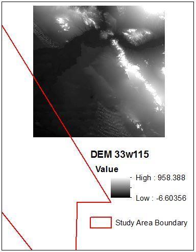
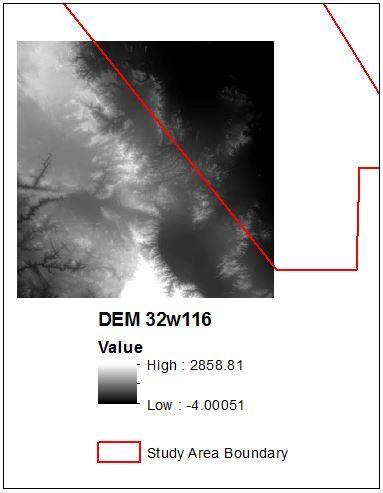
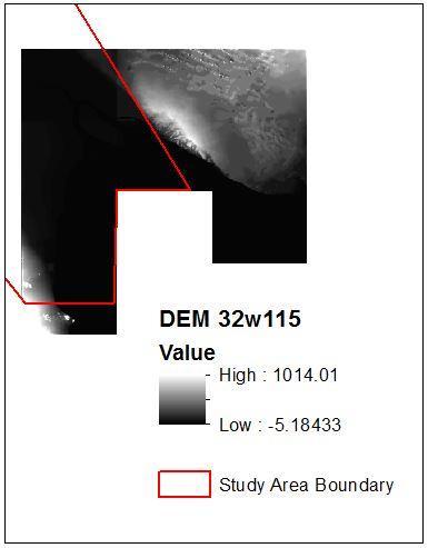
32 Figure 4-2: The DEM Data Collection for Different Regions of the Study Area 15

33 Figure 4-3: The Completed DEM Data for the Study Area The land cover dataset was downloaded from the USGS website, but it only represented the California State. The dataset was clipped for the study area, then modified manually using the Editor tool to cover the Mexican portion of the study area. The land cover of the Mexican portion was digitized from the imagery basemap at the ArcGIS according to the client s request. Figure 4-4 shows the original dataset from the USGS and the result of the final land cover dataset. 16

34 Figure 4-4: The Original Dataset from the USGS and the Completed Land Cover Dataset 4.5 Data Scrubbing and Loading Since the data were collected from websites or provided by the client, data scrubbing was necessary to prepare the data to store into a geodatabase. The road network data were received from the client for California and the Mexicali region in northern Mexico. The data did not have road type, so the Road Type field was created in the attribute table based on the client s knowledge. This field was set up because these data were divided into two datasets using the Select By Attributes tool. The first dataset was for paved roads and the second dataset was for unpaved roads. Figure 4-5 shows the data that were 17

35 provided by the client, and the outcomes data were processed as two datasets. Figure 4-5: The Received Roads Data and the Final Roads Datasets The city and river datasets were received for California and the North Mexico region. They were clipped for the study area using the ArcGIS Clip tool. Furthermore, some undesirable and null value fields were deleted to make the data clean and clear. 4.6 Summary In this chapter, the database design and the associated data to this project were addressed and the logical and conceptual data models were described. Also, the data types and sources were provided as a table. This chapter covered the data preparation to be stored in the geodatabase for this project. 18

36 Chapter 5 Implementation This chapter addresses all the steps that were taken in order to create the project tool to identify the optimal roads for the pipelines and the workflow for the project methodology. Also, this chapter explains the least-cost path analysis that was used to solve the project s problem. Likewise, this chapter discusses weighted overlay analysis to discover the suitable solar sites, followed by a summary at the end of the chapter. 5.1 Factors Analyzed for Pipelines This project has two types of factors: human and natural. These factors were analyzed using the least-cost path approach to create a tool for pipeline routes. The least-cost path analysis is a GIS tool used for connecting two points with a route using the least cost between these two points. The cost could be any criteria available to the user. This tool requires a source point, destination point, and cost surface in a raster format to run correctly. Each cell in the cost surface has a total value that comes from different factors used for a study area. Each factor in this project was analyzed to have the cost surface for this project before running the Least-Cost Path tool Road Factor Roads data were divided by types, paved and unpaved, using the Select Attribute tool. The values for these data were assigned depending on road type. The Euclidean Distance tool was used to calculate the cell values for each road type. The distance for paved roads was 200 meters, while the distance for unpaved roads was 100 meters. Figure 5.1 shows the road distance values, depending on how far the land is from the roads, where the blue color is the farthest from them and the yellow color is the closest to the roads. 19

37 Figure 5-1: Distance Values for the Roads Datasets Using the Euclidean Distance Tool The yellow color has a value of 0 where the roads are. However, this value was changed using the Raster Calculator tool to have the high values on the roads. Positive values were calculated by subtracting 200 from the paved roads values ("%eucdis_paved%" 200) and then multiplied by -1 ("%Paved_200%" * - 1). Similarly, unpaved road values subtracted 100 ("%eucdis_unpaved%" - 100) and then was multiplied by -1 ("%unpaved_100%" * -1) to have positive values. As a result, the 200 and 100 values were assigned where the roads are, and these values gradually decrease down to 0, far from the roads. This process was used because roads are not desirable sites for the pipelines routes; however, the pipeline routes must cross some roads to connect the Salton Sea to the Gulf of California. Figure 5-2 shows the values representing costs across a road. 20

38 Figure 5-2: Roads Values after Changing Using the Raster Calculator Tool The red color represents the highest values, where the roads are, and the green color represents the lower values, which means that the area is far from the roads. These two datasets were put together using the Mosaic To New Raster tool, to have one cost surface for the roads factor. After that, the Raster Calculator tool was used to assign a value of 0 for the areas that do not have roads and are desirable areas for the pipeline routes. Figure 5-3 illustrates the cost surface for roads that was used for the least-cost path method. The workflow in the ModelBuilder to create the project tool is provided in Appendix A-1. 21

39 Figure 5-3: The Cost Surface for the Roads Dataset Slope Factor Slope means how steep a straight line is on the surface. The slope factor was considered because the pipeline routes were applied on the surface. The slope factor was derived from the DEM data using the Slope tool under the Surface tool with the Spatial Analysis toolbox. The slope values in percent rise presented in Figure 5-4 represent the same values that were applied for the slope cost surface. The slope values range from 0, which is most suitable, to 225, which is least suitable. 22

40 Figure 5-4: Slope Factor Values Slope cost values were added to the road cost values using the Raster Calculator tool. As a result, the two factors have the cost surface shown in Figure 5-5, with values ranging from 0 to 282. The lower values are the most suitable and the higher values are least suitable for the pipeline routes. Appendix A-2 shows the workflow to figure out the cost surface for the slope and road cost surface. 23

41 Figure 5-5: Slope and Roads Cost Surface Cities Factor Cities were considered in the study area because they affected where the pipeline routes should be. All cities were given high values in the cost surface since they are not desirable land for building pipelines. The cities dataset was converted to a raster dataset using the Feature to Raster tool. This process was used to put the cities dataset in raster format. After that, the Raster Calculator tool was used with the equation Con(IsNull("%Feature_Cities_Raster%"),0,300) to assign each city with a value of 300 as shown in Figure

42 Figure 5-6: Cost Surface for Cities The result of this process represented the cost surface of the cities where, a value of 300 exemplified cities and a value of 0 was given to a land that is suitable for the pipeline routes. The workflow of this process appears in Figure 5-7. Figure 5-7: Workflow for Cities Cost Surface 25

43 5.1.4 Rivers Factor There are three rivers that cross the study area: Alamo River, New River, and Colorado River. The area for pipeline routes has to be far from the river land. The Buffer tool was used to determine the river buffer area within the 100-meter value range from the river land data as shown in Figure 5-8. After that, the Feature To Raster tool was used to transfer the polyline data to raster data. Afterwards, the raster data was assigned with value of 300 using the Raster Calculator tool and the equation Con(IsNull("%Feature_Rivers_Raster%"),0,300). Figure 5-8: Buffer Map for the River in the Study Area As a result, the cost surface, shown in Figure 5-9, has values of 0 and 300, where 300 means there are rivers and 0 means there are no rivers. The workflow in the ModelBuilder for the rivers factor is shown in Figure These methods were done to give rivers higher values than the land in the study area because the pipeline routes cannot be close to rivers. 26

44 Figure 5-9: The Rivers Cost Surface Figure 5-10: Workflow for Rivers Cost Surface 27

45 5.1.5 Land Cover Factor The study area has different types of land cover, and all of these types appear in Table 5-1. Some of them were assigned with high values on the cost surface based on the client s needs. However, some cover types were assigned with low values because they did not affect the pipelines routes. Table 5-1: Land Cover Types and Their Values ID Number Land Cover Type Values based on the Client s Needs 1 Desert Scrub 1 2 Cropland Desert Wash 1 4 Annual Grassland Lacustrine Desert Succulent Shrub 1 7 Urban Juniper

46 A value of 300 means undesirable lands for pipelines, while a value 1 means desirable land for pipelines. Each of the cover types was assigned with a value and an ID number to be used in the processing tool. The workflow for the land cover had two steps, shown in Appendix A-3. The first step is converting the Land Cover dataset to raster format, using the Feature To Raster tool. The second step was to assign the land cover types with their values using the Raster Calculator tool (Figure 5-11). The expression used the ID number that represented each land cover type and assigned it with its value. Figure 5-11: Raster Calculator for the Land Cover Types As a result of this calculation, the cost surface of land cover was created (Figure 5-12) as the final work on the land cover dataset. 29

47 Figure 5-12: The Cost Surface for the Land Cover Dataset Protected Land Factor The land north of the Gulf of California is protected, as is the Colorado River Delta. This area is protected to save the delta from any kind of influence by the pipelines. The data were in polygon factor type, so the Feature To Raster tool was used to convert it to raster data type. After that, the Raster Calculator tool was used to add high value to the protected land because the pipeline routes con not go there. The equation in Figure 5-13 was used to assign a value of 300 to the protected land dataset. 30

48 Figure 5-13: The Equation to Convert the Protected Land Dataset The result of this equation was the cost surface of the protected land factor, as shown in Figure Also, the workflow for the protected land factor is presented in Appendix A-4. Figure 5-14: The Cost Surface for the Protected Land 5.2 Least-Cost Path Analysis The least-cost path needs three factors as inputs in order to run correctly. The three factors are the feature source data, feature destination data, and cost surface in raster format. The source and destination data were given by the client as point feature classes. 31

49 The cost surface was derived from the factors discussed in Section 5.1. Each factor has a cost surface, and they were added together to create one cost surface using the Raster Calculator tool (Figure 5-15). Figure 5-15: The Workflow for the Main Cost Surface There are two steps for the least-cost path analysis: determining the cost distance and finding the cost path (shown in Figure 5-16). The cost distance requires three inputs: feature source data, cost raster, and output distance raster. On the other hand, the cost path requires four inputs: feature destination data, cost distance raster, cost backlink raster, and output raster. The first step was to determine the cost distance, where the cost surface and start point datasets were used as inputs. The output of the cost distance was used as an input for the cost path step. Also, the cost backlink was derived from the cost distance process as a second input for the cost path. The third input was the end point dataset, and the final input was the output raster file. The final output was the final suitable path in a raster format. The Raster To Polyline tool was used to convert a raster dataset to a feature dataset. As a result, the raster suitable path was converted to polyline feature class. The final output was the pipeline routes in polyline feature class, the main goal of this project. 32

50 Figure 5-16: The Workflow for the Least-Cost Path Method 5.3 Preparing Datasets for Solar Sites Analysis Solar sites were required around the pipelines at high-elevation areas. To identify the study area for the solar sites, the elevation profile was created. The elevation profile was developed using the pipeline route dataset. The pipeline data were converted to 3D data by using the Interpolate Shape tool with the 3D Analyst tool. After that, the Profile Graph tool was used to draw the pipeline elevation profile (see Figure 5-17). From the elevation profile, there are two peak areas. The first peak area has 60-meter elevation, and the second peak area has 20-meter elevation. The 60- and 20-meter elevation datasets were derived from the original DEM dataset. These datasets were converted to feature class using the Raster To Polygon tool. After that, the Intersect tool was applied to select the pipeline routes that cross these elevation values. These routes were used to generate a buffer of 500 meters according to the client s needs. The outputs of these steps were the study areas for the solar sites. Moreover, these study areas were used to develop the DEM for them by using the Clip tool. As a result of these processes ( see Appendix B-1), the study areas, DEMs, and pipeline route datasets were available for factors analysis. 33

51 Figure 5-17: Pipeline Elevation Profile (Vertical = elevation in meter, Horizontal = distance in meter) 5.4 Weighted Overlay Analysis for Solar Sites Weighted overlay analysis is one of the most common methods used for suitable solar sites. This method needs different factors in a raster format. These factors should be weighted according to their importance. Also, they should have a common measurement scale to determine which is most suitable. The output of this analysis delivers classified suitable values in a raster format. Three factors were needed in this project to fit the client s needs. Slope, solar radiation, and distance from the pipelines were the factors for this project. Each factor went through a process before they were put together in the Weighted Overlay tool. The slope factor was derived from the original DEM, as shown previously in Appendix B-1. The Slope tool was applied on both DEMs for the 60- and 20-meter elevation areas. After that, the Reclassify tool was used to reassign the slope values to new values using equal interval method, as shown in Table 5-2. The classified new values were ranged between 10 1, where 10 was the most suitable and 1 was the least suitable. The slope factor was weighted 25% influence in the Weighted Overlay tool (Figure 5-18). 34

52 Table 5-2: Slope Factor Reclassification Class Slope Values Reclassification Values 1 < Figure 5-18: Influence and Values for the Slope Factor The solar radiation factor data was loaded from the DEM by using the Area Solar Radiation tool. This tool calculates how much sun light is received during a period of time at a specific location on Earth according to elevation, orientation, and shadows. The value range was between kilowatt-hours per square meter per day (kwh/m²/day) for both elevation areas. Since these values were in suitable area for solar sites according to the client s knowledge, they were divided to 6 classes based on the solar radiation values by using the Reclassify tool. As a result, the reclassification range was between 5 to 10, where 10 was the most desirable and 5 was the least desirable (see Table 5-3). The radiation factor was weighted 50% influence in the Weighted Overlay tool (Figure 5-19). 35

53 Table 5-3: The Reclassification for the Solar Radiation Factor Class Solar Radiation Values in (kwh/m²/day) Reclassification Values 1 < < Figure 5-19: Influence and Values for the Solar Radiation Factor The distance from the pipelines was determined from the pipelines dataset that was created from the least-cost path output. The Euclidean Distance tool was used with 500-meter maximum distance to divide the area based on the distance from the pipelines. The output values were divided into 10 classes and reclassified into a range of 1 to 10 by using the Reclassify tool. The equal interval method was used to reclassify each class by 50 meter, as shown in Table 5-4. The area closest to the pipelines had a value of 10, while the area farthest from the pipelines had a value of 1. The distance to pipeline factor was weighted 25% in the Weighted Overlay tool (Figure 5-20). Table 5-4: The Reclassification for the Distance to Pipelines Factor Class Distance to Pipelines Values in Meter Reclassification Values

54 Figure 5-20: Influence and Values for the Distance from the Pipelines Factor The three factors for each study area were calculated in the same way as discussed above (Appendix B-2). The outputs of the weighted overlay were the final outcomes as the most suitable areas for solar sites around the pipelines. 5.5 Summary The implementation chapter discussed the methodology that was applied in this project to reach the final outcomes. The least-cost path and weighted overlay analysis steps were explained in this chapter for better understanding. 37

55

56 Chapter 6 Results and Analysis The final result of this project was a map that represents the pipeline routes and suitable sites for solar energy farming. There are three tools that were created to reach the project s goals. All of these tools were developed via ModelBuilder in ArcGIS The pipelines tool and map discussed in section 6.1. Section 6.2 explains the criteria of the solar sites tools and maps. Section 6.3 discuses different scenarios that applied on this project, followed by a summary that concludes this chapter. 6.1 Pipelines Map and Tool The main goal of this project was to determine optimal routes for pipelines. The route was generated considering human and natural factors to reduce the environmental impacts. A tool and map were developed to achieve this goal. The tool helped to determine the factors and analysis that have to be done for this project (Figure 6-1). 39

57 Figure 6-1: The Final Analysis Tool for Pipelines This diagram shows the step-by-step processes to create the final map that was requested by the client. The final route was in a polyline feature dataset format that was editable. This map displays the best pipeline routes between the Salton Sea and the Gulf of California (Figure 6-2). 40

58 Figure 6-2: Proposed Optimal Location for Pipelines The pipeline route s length was about 280 kilometers, with a distance of 78 km in California and a distance of 202 km in Mexico. This route started at 68 meters below the sea level at the south of Salton Sea City and reached 60 meters above sea level at the highest elevation point when it crossed the Sierra Cucapah mountains. Afterward, the 41

59 route extended to Laguna Salada Lake, where the elevation is near sea level. The final destination of this route was at the Gulf of California, north of San Felipe City, Mexico. 6.2 Solar Sites Maps and Tool The solar sites were required by the client to be close to the pipeline routes. The solar sites were located in high-elevation areas to provide electricity for pumping water from the lower elevation and saving energy for the future. There were two high elevation areas located around the Sierra Cucapah mountains. The first of these areas was 60-meter elevation and the second was 20-meter elevation. As a result, a tool with the same factors for both areas was developed to determine the most suitable land for solar sites that were adjacent to the pipelines, as shown in Figure 6-3. Figure 6-3: The Solar Site Tool for 60 and 20-Meter Elevation Areas Slope, solar radiation area, and distance from pipelines were the factors that were analyzed for both areas. The analysis revealed the most suitable land for solar sites for both areas as shown in Figures 6-4 and

60 !! PipeIines Most Suitable Least Suitable Figure 6-4: Suitability Surface for Solar Sites at the 60-Meter Elevation Area 43

61 !! PipeIines Most Suitable Least Suitable Figure 6-5: Suitability Surface for Solar Sites at the 20-Meter Elevation Area 44

62 The green color signifies land that is suitable for solar farms, while the red color represents unsuitable land for solar farms. Both of these areas were added to the pipelines map to produce the final map for this project, shown in Figure 6-6. Figure 6-6: Pipelines and Solar Sites as the Final Map for this Project 45

63 6.3 Discussion This section discussed several ideas that were applied in this project. These ideas came from different logical prospects related to this project. The project s can be modified so that the user could change the factor criteria of this project. For instance, the road factor criteria was changed to consider the logistics of constructing pipelines. It is more desirable that a pipeline is close to a road, but not cross a road. This idea was applied on the project for easy access and supporting the maintenance and construction equipment on the pipelines. The cost value was 200 where the roads are and gradually decreased to 1 at a distance of 200 meters. The cost values then increased until reaching a cost value of 300 at a distance of 1000 meters and beyond. Figure 6-7 shows the relation between the cost and the distance to a road. Figure 6-8 presents the optimal route for pipelines when the new road cost surface was applied. It can be seen that the route generally follows the road network. Figure 6-7: The Relations between the Cost and the Distance to a Road 46

64 Zoom in to a road Figure 6-8: Cost Surface for the Pipeline Routes Close to the Roads Another example was to assign the protected area with higher value because it is prohibited land that the pipeline routes cannot go there. Also, the land close to the protected area is not desirable to build the pipelines. As a result, the protected area factor dataset was assigned with 500 cost values. After that, a buffer of 300 meter was applied on the protected area. The buffer cost value was 200 which means the land next the 47

65 protected area is also not suitable for pipeline routes. After the cost surface was changed, the optimal route was generated again and illustrated in Figure 6-9. But there was no different between this road and the previous one in Figure 6-8. This is due to the dominant influence of the road factor. Figure 6-9: The High-Cost Surface Values for the Protected Area 48

66 If planers think land cover factor should not be included, it can be easily removed from the analysis. When this happened, the roads for pipelines was changed as demonstrated in Figure Figure 6-10: The Cost Surface without the Land Cover Factor 49

67 6.4 Summary The final outcomes of this project were explained in this chapter. The pipeline tool and map were reviewed at the beginning of this chapter. Also, the solar sites tools and maps were discussed, followed by a single map combining the pipelines and solar sites as the final map of this project. Different scenarios in constructing the cost surface for routing were also applied. 50

68 Chapter 7 Conclusions and Future Work This chapter describes the project conclusion in section 7.1. Also, the future work (section 7.2) suggests some ways of improving this project. Lastly, a summary of this chapter is provided. 7.1 Project Conclusion This project established how to find optimal locations for pipelines and apply solar sites around the pipelines, which were the main goals of this project. Some factors were considered in accordance with the client s request. These goals were achieved by using ArcGIS and ModelBuilder to create maps and tools for this project. The first map was created to represent the pipeline routes between the Salton Sea and the Gulf of California. Furthermore, a tool was developed to identify the best location for pipelines using the least-cost path method, while weighted overlay analysis was used to discover where best to put the solar sites. As a result, the second map was developed to show the suitable land for solar sites at 60-meter elevation around the pipelines. Similarly, the last map was generated to designate suitable land for solar sites at 20-meter elevation. All these maps and tools were presented to the client, Dr. Timothy Krantz, to prove the final outcomes of this project. 7.2 Future Work This project can be improved by following different recommendations. These recommendations include improving the DEM data, adding more factors, developing a web application, and creating an active toolset. The DEM data was in 30-meter resolution for this project. One way to improve this type of project is to perform researches for DEM data that has 10-meter resolution and apply this data to the pipelines tool. This data could improve the accuracy of the elevation values and the pipeline routes. However, this data will make processing slower for a large study area such as in this project. To solve this problem, the study area could be divided into different regions and then use different tools developed for each area. This suggestion would improve the DEM data for future work on this project. Another suggestion for future work on this type of project is to include more factors for pipeline and solar site tools. Nine factors were used for both tools; however, it is possible to add more factors to the tools. For example, streams and land-use with ownership fields. The streams dataset could be used for finding pipeline routes and suitable solar sites. A condition of using this dataset would be that if there is a stream, pipeline routes change their direction and the stream land is not suitable for solar sites. The land-use dataset uses the ownership field with two classes. The first class is government ownership, which means accessible land for pipelines and solar sites. The second class is private ownership, which means land that is inaccessible for pipelines and solar sites. These datasets could be hard to find on the open source websites for the public. 51

69 Using web GIS application is the third suggestion of this project. This project could be published using ArcGIS Online or Esri Story Maps applications. The first goal of using such an application is depicting the pipeline routes with some pop-up information about the pipelines. The second goal is to display some of the solar sites around the pipeline. Additionally, the developer could present some charts or diagrams about the pipelines and solar sites statistics. Also, some functions could be added to the application that a user could operate to understand the application. The last suggestion is to create an active toolset using the tools provided in this project. Making an active toolset means developing some geoprocessing tools using ModelBuilder and the Python programming language to let users process their datasets. This toolset should draw pipeline routes for any geographic study area that the users want. Also, this toolset should have several entry factors that the developer would determine for the users. This suggestion could be used in a long-term project for developers who are interested in water resources. 52

70 Works Cited Bail, K. M. (2015). Salton Sea and Salinity. Retrieved from Imperial County: Chandio, A. N., Matori, A. B., WanYusof, K. B., Talpur, M. H., Khahro, S.H., & Mokhtar, M. R., (2012). Computer Application in Routing of Road using Least- Cost Path Analysis in Hillside Development. Research Journal of Environmental and Earth Sciences, 907. Esri. (2012, August 11). Understanding solar radiation analysis. Retrieved from ArcGIS Resources: Feldman, S. C. (1995, August). A Prototype for Pipeline Routing Using Remotely Sensed Data and Geographic Information. Retrieved from Science Direct: Kelly, A. (2014, May 10). GIS Least-Cost Route Modeling of the Proposed Trans- Anatolian Pipeline in Western Turkey. Retrieved from Georgia State University: Kuo, L. (2014, March 07). China Has Launched the Largest Water-Pipeline Project in History. Retrieved from The Atlantic: McKinney, M. (2014). Site Suitability Analysis for Solar Farm in Watauga County, NC. Boone: Appalachian State University. Mick, R. & Teykl, K., (2015). GIS-ENABLED: Modeling Simplifies Pipeline Route Selection. Retrieved from Water World: 4/departments/automation-technology/gis-enabled-modeling-simplifies-pipelineroute-selection.html Orr, A. B. (2011). Mojave Desert Ecosystem Program Solar and Wind Energy Suitability Modeling Tools. Redlands: University of Redlands. Topal, T. a. (2009, April). Geotechnical Assessment of A Landslide Along A Aatural Gas Pipeline for Possible Remediations (Karacabey-Turkey). Retrieved from Environmental Geology: #page-1 53

71

72 Appendix A. Workflow for Pipeline Factors This appendix contains the workflow that were done in ModelBuilder for determine the pipeline routes. Figure A-1: The Road Factor Workflow Figure A-2: Slope Factor Workflow with Road Factor 55

73 Figure A-3: The Workflow for the Land Cover Figure A-4: The Workflow for the Protected Land Factor 56

74 Appendix B. Workflow for Solar Site Factors This appendix contains the workflow that were done in ModelBuilder for discovering the solar sites around the pipeline routes. Figure B-1: Steps for Preparing Datasets for Solar Sites Analysis 57

75 Figure B-2: The Three Analyzed Factors for the Solar Sites 58