Investigating the Potentiality of Regression Kriging in the Estimation of Soil Organic Carbon Versus the Extracted Result from the Existing Soil Map

Transcription

1 Investigating the Potentiality of Regression Kriging in the Estimation of Soil Organic Carbon Versus the Extracted Result from the Existing Soil Map Navneet Kumar January, 2009

2 Investigating the Potentiality of Regression Kriging in the Estimation of Soil Organic Carbon versus the Extracted Result from the Existing Soil Map By Navneet Kumar Thesis submitted to the International Institute for Geo-information Science and Earth Observation in partial fulfilment of the requirements for the degree of Master of Science in Geo-information Science and Earth Observation, Specialisation: Geoinformatics Thesis Assessment Board Thesis Supervisors Chairman : Prof. Dr. Ir. A. (Alfred) Stein IIRS : Dr. A. Vel Murugan External Examiner : Dr. Anil Rai : Dr. S.P. Aggarwal IIRS Member : Dr. A. Vel Murugan ITC : Dr. Abbas Farshad IIRS Member : Dr. S.P. Aggarwal : Dr. Nicholas Hamm IIRS Member : Mr. P.L.N. Raju IIRS Member : Dr. Sameer Saran iirs INTERNATIONAL INSTITUTE FOR GEO-INFORMATION SCIENCE AND EARTH OBSERVATION ENSCHEDE, THE NETHERLANDS & INDIAN INSTITUTE OF REMOTE SENSING, NATIONAL REMOTE SENSING CENTRE (NRSE), ISRO, DEPARTMENT OF SPACE, GOVT. OF INDIA, DEHRADUN, INDIA

3 Disclaimer This document describes work undertaken as part of a programme of study at the Indian Institute of Remote Sensing and International Institute for Geo-information Science and Earth Observation. All views and opinions expressed therein remain the sole responsibility of the author, and do not necessarily represent those of the institute.

4 Dedicated to My Parents

5 Abstract A hybrid spatial prediction technique for soil organic carbon based on multiple regression and kriging is described and compared with conventional soil map. Five different types of sampling designs were also tested for a part of the study area to predict soil organic carbon in a cost effective manner using regression-kriging technique. The study area is a sub watershed under Solani watershed located in western Utter Pradesh, India. In the present study soil organic carbon (target variable) was predicted using eight predictor variables. The soil organic carbon was determined in 248 soil samples which were collected by random sampling within a 300m 2 grid overlaid on the study area. Out of which 212 soil samples were used for regression analysis and rest of the samples formed the validation data sets. The same soil samples were used to evaluate different sampling design viz., square, rectangle, triangle, stratified and random sample within a grid sampling. The target variable was first logit transformed to have normal distribution and standardised principal component analysis of predictor variables was done to remove multicollinearity. The target variable was fitted using step-wise regression and regression residuals are modelled as residual variogram, later it was added with the trend to get the final overall prediction results. Out of the eight predictor variables used in simple regression, NDVI has the maximum correlation with the soil organic carbon (0.64) followed by VTCI (0.60), Brightness index (-0.60), Greenness index (0.57) and wetness index (0.51). The regression kriging predicted SOC value ranges from 0.19 to 2.03 % with a mean value of 0.64 and standard deviation of The values are higher in upper piedmont with moderate forest followed by Siwalik hills while low values are found in the upper alluvial plains. The F statistics and p value indicated that the prediction results are highly significant. Further, RMSE value is lower for regression kriging predicted map (0.19) than conventional SOC map (0.28) which indicates that regression kriging predicted SOC values are much closer to the observed values. It is also observed that random sample within a grid is a better design than others as it was found to have lower RMSE value (0.144) and mean error (-0.002) than other designs. When the cost of collection, analysis and mapping is compared, conventional SOC map is much cheaper but it represents discrete units. However, regression kriging predicted SOC map is an ideal input for spatially distributed models and the higher cost of is justified when quality, spatial distribution and accuracy are considered. So, it can be concluded that regression kriging predicts SOC even with the mapping units used in conventional soil maps and it can also be used to upscale the point measurements to a much larger area in a spatially distributed manner. Keywords: Logit transformation; Standard principal component analysis; Environmental correlation, Spatial prediction; Semi variogram. i

6 Acknowledgements One of the most sanguine part of the completion of an endeavour is to extend sincere gratitude to all those who have been explicitly or implicitly involved in the project. First of all, I would like to express my deepest sense of gratitude to my supervisors Dr. A.Vel Murugan and Dr. S.P. Aggarwal for their patient guidance and excellent advice throughout this study. Their co-operative attitude has made accomplishment of this research work well in time. I would like to record my gratitude to Dr. Abbas Farshad and Dr. Nicholas Hamm (ITC) for their supervision, advice, and guidance from the very early stage of this research as well as giving me extraordinary suggestions throughout the work. I am immensely grateful to Dr. V.K. Dadhwal, Dean, Indian Institute of Remote Sensing (IIRS), Dehradun, the force behind the credibility of this premier International level Institute where I got privilege to be a learner. I am highly thankful to Mr. P.L.N. Raju, In-charge, Geoinformatics division and Dr. Sameer Saran, Programme coordinator, Geoinformatics course for their support and encouragement. My Sincere thanks to all the fellow participants of Geoinformatics and Geo-hazards course. I will always remember my friends Jitendra Dixit, Anurag Verma, Rahul Raj, Shashi Kumar, Kumar Gaurav and M.K. Beg for their kind support and cooperation throughout my stay in IIRS. I will never forget the life we have enjoyed together in Europe. I am also thankful to my seniors Bikash Ranjan Parida, Sekhar LukoseKuriakose and Rishi Raj Dutta for their valuable suggestions. Last but not least, my sense of acknowledgements will remain incomplete, if i forget the efforts and consistent moral support of my parents and brothers Prashant and Vivek. ii

7 Table of contents 1. Introduction Background Problem statement... 2 Research objectives General Research Objectives Secondary and Related Objectives Research Questions Research Hypothesis Literature Review Introduction Soil Organic Carbon Importance of Soil Organic Carbon in Agriculture Factors Affecting SOC and its Distribution Soil Mapping Geostatistics Stationary hypothesis Kriging Ordinary Kriging Prediction Variance Regression Kriging (Hybrid Interpolation Technique) Difference between regression kriging, kriging with external drift and universal kriging Advantages of regression kriging Predictor variables Seasonal mean NDVI Tasseled cap indices Vegetation temperature condition index (VTCI) Topographic attributes Previous studies on prediction Traditional soil classification era of ignorance (the dark ages) Spatial classification and prediction from soil maps era of classical statistics Soil geostatistics era of enlightenment (modern statistics) Summary of the previous studies Sampling Design Study Area Location and Extent of Sub Watershed Climate Humidity Geology Drainage Physiography iii

8 3.7. Natural Vegetation Materials and Methods Data collection The Prediction approach Preparation of different input variables Methods to predict SOC in the entire study area Evaluation of sampling designs in part of study area (in agriculture land) Target variable (variable that will be spatially predicted) Soil sampling for the entire study area Soil sampling for a part of study area (agricultural land) Laboratory analysis of soil samples Predictor variables Geo-referencing and dataset generation Bring all the input dataset to 30 m resolution Derive DEM Derive Slope in percentage map Calculate the Compound topographic index (CTI) Derive Seasonal Mean NDVI Derive the tasseled cap indices Compute the Vegetation temperature condition index (VTCI) in ENVI Preparation of soil organic carbon map Regression kriging a hybrid interpolation technique Computational steps involved: Validation Mean error (ME) Root Mean Square Error (RMSE) Sampling design validation Comparison between regression kriging predicted map with conventional soil organic carbon map Results and discussion Analysis of Target variable Analysis of Predictor variables Regression Analysis Simple regression analysis Multiple regression analysis Principal component analysis Analysis of Residuals Residual Histogram Variogram modelling of residuals Spatial prediction Predicted SOC Validation Comparison of conventional SOC map with regression kriging predicted map Sampling design Design validation Conclusions and recommendations iv

9 References Annexures Appendix Appendix Appendix Appendix v

10 List of figures Figure 2-1: (a) & (b) are showing three different axis of tasseled cap transformation (TCT) Figure 3-1: Study Area Figure 3-2: Mean Monthly Climate Data (Source: Meteorological Station, Roorkee) Figure 4-1: Showing the processing steps of different input variables Figure 4-2: Flow chart- Describes the different steps during the research work for the entire area Figure 4-3: Methodology 3 Flow chart: Describes the different steps during the research work for a part of study area Figure 4-4: sample point location of interpolation soil samples Figure 4-5: Square sampling design Figure 4-6: Rectangular sampling design Figure 4-7: Triangular sampling design Figure 4-8: Figure Stratified sampling design Figure 4-9: Random sample with a grid sampling design Figure 4-10: Flow chart showing steps to compute tasseled cap transformation (TCT) Figure 4-11: Parameterization of LST NDVIimax and LST NDVIimin from LST/NDVI triangle Figure 5-1: Histogram of measured SOC values Figure 5-2: Histogram of Logit transformed SOC values Figure 5-3: Box plot of measured SOC Figure 5-4: Box plot of Logit transformed SOC Figure 5-5: QQ plot of measured SOC values Figure 5-6: QQ plot of logit transformed SOC values Figure 5-7: Brightness index Figure 5-8: Greenness index Figure 5-9: Wetness index Figure 5-10: Seasonal mean NDVI Figure 5-11: VTCI Figure 5-12: DEM Figure 5-13: Slope in percentage Figure 5-14: Compound topographic index Figure 5-15: Individual correlation plots of different significant Standard principal components (SPCs) with Soil organic carbon Figure 5-16: Residual histogram Figure 5-17: Empirical variogram Figure 5-18: Modelled Variogram Figure 5-19: (a) Logit transformed Predicted SOC and (b) Back transformed Predicted SOC Figure 5-20: Kriging variance Figure 5-21: Comparison between (a) Regression kriging predicted SOC map and (b) Conventional soil organic carbon map Figure 5-22: Square sampling (a) Predicted SOC and (b) Kriging variance Figure 5-23: Rectangular sampling (a) Predicted SOC and (b) Kriging Variance Figure 5-24: Triangular sampling (a) Predicted SOC and (b) Kriging Variance Figure 5-25: (a) Predicted SOC and (b) Kriging Variance Figure 5-26: Random Sample within a grid (a) Predicted SOC and (b) Kriging Variance vi

11 List of tables Table 2-1: Showing ASTER coefficients for tassel cap transformation Table 2-2: Showing summary of few relevant studies on prediction (with Author and year) Table 2-3: Shows the comparison of prediction accuracy of different spatial prediction techniques (with Author and year) Table 4-1: Secondary data used Table 4-2: Predictor variables Table 4-3: KT coefficients Table 4-4: Soil mapping units and SOC values extracted from the soil map Table 5-1: Summary statistics of target variable (Interpolation dataset) Table 5-2: Correlation matrix of different predictor variables with soil organic carbon Table 5-3: Beta values of different predictor variables (Individual effect) Table 5-4: Summary statistics of multiple regression analysis Table 5-5: Coefficients of different predictor variables (Multiple regression analysis) Table 5-6: Correlation matrix of predictor variables Table 5-7: Coefficients of SPC components after step wise regression analysis Table 5-8: Summary of validation of SOC predicted by regression kriging Table 5-9: Comparison of two different techniques Table 5-10: Summary statistics of SOC values used in different sampling designs Table 5-11: Summary of predicted SOC in different sampling designs Table 5-12: Summary of validation results for different sampling designs vii

12 List of abbreviations. B.I. Brightness index CTI Compound topographic index GAM General additive modelling. G.I. Greenness index IDP Inverse distance to a power. KED Kriging with external drift KT Kauth-Thomas LOOCV Leave one out cross validation LR Linear regression ME Mean error MLR Multiple linear regression MR Multiple regression NDVI Normalized difference vegetation index NIH National institute of hydrology OK Ordinary kriging RK Regression kriging RI Relative improvement RMSE Root mean square error RT Regression tree SK Simple kriging SOC Soil organic carbon SSR Square sum of residuals SWIR Short wave infra red TCT Tasseled cap transformation TIR Thermal infra red UK Universal kriging VNIR Visible near infra red VTCI Vegetation temperature condition index W.I. Wetness index viii

13 1. Introduction 1.1. Background Sustainable land management requires reliable information on the spatial distribution of soil properties affecting both landscape process and services. The concepts of sustainable agriculture put emphasis on the management of soil organic matter for maintaining soil fertility (shibu et al., 2006). Maps of soil organic carbon is of interest for agricultural management as well as in environmental research related to terrestrial sequestration of atmospheric carbon. Also digital mapping of soil organic carbon (SOC) is important for site specific crop management (Dobermann and Ping, 2004). Geostatistical tools have been applied to study the spatial distribution patterns, quantification and changes in soil organic carbon (Van Meirvenne et al., 1996; Saldana et al., 1998; Chevallier et al., 2000; Frogbrook and Oliver, 2001). Some authors believe that geostatistical methods are superior over other estimation methods, such as polynomial interpolation, thiessen polygon and inverse distance method (Creutin, 1982; Tabios and Salas, 1985). In conventional soil survey soil properties are recorded at representative sites and assigned to entire mapping unit, which are delineated following one of the physiographic, physiognomic and geopedologic approaches. Although soil surveyors are very well aware of the spatial variability of soil properties, conventionally prepared soil maps do not reflect it as soil units are limited by boundaries (Heuvelink and Webster; 2001). But in nature the soil properties are highly variable spatially (Burrough, 1993) and for accurate estimation of soil properties these continuous variability should be considered. In the 1970s a new technique called kriging and its variants were widely recognized as an important spatial interpolation technique in land resource inventories (Hengl et al., 2004). The traditional method of soil analysis and interpretation are laborious, time consuming, hence becoming expensive. Later in the 1990s, with the advancement of GIS and remote sensing technology, predictive soil mapping techniques were introduced. Using inexpensive and readily available ancillary data and indicators that reveal a close relationship to specific soil quantities were used for spatial interpolation (Hengl et al., 2004). The approach was also termed as environmental correlation by McKenzie and Ryan (1999). A number of studies were carried out which considers the multiple regressions of soil organic carbon with auxiliary variables for spatial prediction e.g. terrain indices (Muller and Pierce, 2003) or remote sensing (Lark, 2000). At present the rapid development and intension of scientists to give more precise estimation has given birth to hybrid technologies. Hybrid interpolation techniques, combines both kriging and ancillary data. This proved to give better prediction results than using single approach (Bishop and McBratney, 2001; Bourenane and King, 2003; Lloyd, 2005). One of these hybrid interpolation techniques is known as regression kriging (RK) (Hengl et al., 2004). 1

14 Hengl et al. (2004) and Sumfleth et al. (2008) concluded that regression kriging is becoming popular nowadays because of its better prediction accuracy over different regionalization techniques, such as multi linear regression, simple kriging, inverse distance to power, ordinary kriging. Several authors (Hengl et al., 2007) have been mentioned the strength and limitations of regression kriging techniques. It is important to investigate in what circumstances and situations regression kriging provides the best prediction results in minimum number of field samples. Attention is also been paid to soil sampling, as the conventional soil survey is considered time consuming, laborious and costly (Webster and Olivier, 1990). So, sampling strategy should be designed to get maximum information about reality from a small portion of it, with a minimum of cost and effort. Hence, it is of prime importance to investigate the role of different auxiliary variables and other factors which makes regression kriging superior over others with best sampling design Problem statement In India majority of soil maps were prepared by conventional methods and a very few work has been done so far to use the modern spatial prediction techniques in this regard. The accurate estimation of spatial distribution of soil organic carbon is important in precision agriculture and is one of the basis for decision and policy makers to make plans and strategies. Despite having the knowledge of the SOC s importance, studies related to the relationship between the spatial variation of the SOC and environmental factors are few (Venteris et al., 2004). How to achieve accurate estimation of SOC concentration using the best prediction geostatistical method is a pressing need of the hour. However, a few studies have attempted to work on establishing the relationship between tasseled cap indices and compound topographic index (CTI) with soil organic carbon, and then predicting SOC using regression kriging has been done till now. Again until i have not come across any paper which has mentioned about the relationship of vegetation temperature condition index (VTCI) with soil organic carbon. So, my aim is to address the above mentioned problems through my research work. Research objectives General Research Objectives To spatially predict soil organic carbon for a heterogeneous landscape using the regression kriging in cost effective manner. To evaluate the prediction quality of the regression kriging against the result extracted from the available (conventionally prepared) soil map of the area. 2

15 Secondary and Related Objectives To establish relationship between the different terrain attributes (DEM, CTI and Slope), tasseled cap indices, vegetation temperature condition index (VTCI) and seasonal mean NDVI with the soil organic carbon content (regression). To reclassify the conventional soil map and prepare soil organic carbon map. To bring all the data on the same support (grid size). To compare the two final prediction maps in GIS environment Research Questions Is it possible to spatially predict the distribution of soil organic carbon by regression kriging technique in a cost effective manner? How accurate is the prediction of soil organic carbon based on regression kriging to the field / lab data and the results extracted by conventional soil map? How the selected variables are related to soil organic carbon? How to bring dataset from different sources in same grid size? How to compare the two final prediction maps in GIS environment? 1.4. Research Hypothesis NDVI and Compound topographic index (CTI) is having a spatial relationship with soil organic carbon and can be used as predictors in regression kriging model. 3

16 2. Literature Review 2.1. Introduction Researchers and policy-makers need accurate and consistent methods for the estimation of spatial distribution of soil organic carbon. Spatial variation in soil has been recognised for many years (Burrough, 1993). Geostatistics has been applied in soil science for more than 20 years and has provided modern techniques to quantify the spatial soil parameters and performed spatial interpolation (Burgess and Webster, 1980 and Webster, 1994). To quantify the distribution of spatial patterns and changes in soil organic carbon, geostatistics has been applied (e.g., Van Meirvenne et al., 1996; Saldana et al., 1998; Chevallier et al., 2000; Frogbrook and Oliver, 2001). Many previous studies have pin pointed the potentiality of exhaustive auxiliary data such as terrain indices (Muller and Pierce, 2003) or remote sensing (Lark, 2000) for producing more precise and accurate maps of soil organic carbon or soil organic matter. The spatial distribution of SOC is generally consistent with elevation and precipitation (McGrath et al., 2003). Burgess and Webster (1980) were the first to use kriging and its practical application, in soil survey, later many other pedologists and environmental scientists have followed it in their literature. Many authors (Goovaerts, 1999 and Webster and Oliver, 2001) have written excellent accounts of geostatistics and its underlying concepts for soil scientists. Geostatistical methods which consider environmental correlation in prediction include cokriging, kriging within strata, kriging with external drift, and regression kriging (Goovaerts, 1997; Odeh et al., 1995). In light of geostatistics many hybrid techniques have been evaluated for their prediction accuracy. One of such hybrid geostatistical techniques is regression kriging which is gaining popularity now a day for its better prediction accuracy over others. Hybrid techniques generally results in more accurate local predictions than ordinary kriging or other univariate predictors. (Goovaerts, 1999; McBratney et al. 2000; Odeh et al., 1995; Triantafilis et al., 2001). Hengl et al., 2004 and Sumfleth et al., 2008 concluded that regression kriging have more accurate prediction over different regionalization techniques, such as multi linear regression, simple kriging, inverse distance to power and ordinary kriging Soil Organic Carbon Soil organic carbon (SOC) is the carbon associated with soil organic matter. Soil organic matter (SOM) constitutes the organic fraction of soil; it is composed of decomposed flora, fauna and microorganisms but does not include un-decomposed plant materials such as litter and straw. Soil organic carbon is expressed as a percentage by weight (g C/kg soil). SOC is closely related to the amount of soil organic matter in the soil. To convert SOC (measured in laboratory) to soil organic matter (SOM), the simple equation SOC x 1.72 = SOM is used. Bulk density would be needed to calculate SOM of soil/volume, for instance, per cubic meter. Soil organic carbon is a dynamic component of the terrestrial system, which changes both internally (in vertical and horizontal directions) and externally with the atmosphere and biosphere (Chan, 2008). 4

17 Importance of Soil Organic Carbon in Agriculture Soil organic carbon is a major determinant and indicator of soil fertility and is highly related to crop productivity (Jia et al., 2007). It improves the physical, chemical and biological properties of soil, enhances the water holding capacity and structural stability, provides aeration to plant roots and microorganisms, binds the nutrients for plant uptake, increases the cation exchange capacity (CEC), and provides organic acid that makes minerals available to plants and buffers soil from strong changes in ph. Hence, maintaining the overall biological health of soil. SOC content below 1% creates problem to obtain potential crop yields with sustainability, also SOC less than 2% makes soil aggregates unstable (Korschens et al., 1998) Factors Affecting SOC and its Distribution Land use, climate, topography and soil type mainly affect the soil organic carbon pools directly through residue and manure inputs, and indirectly by influencing decomposition rates. The soil organic carbon (SOC) content depends largely on soil management practices and quality of organic restitution to the soil (Chan, 2008). SOC is having positive correlation with silt-plus-clay, negative correlation with sand and insignificant correlation with ph (McGrath et al., 2003). The anthropogenic activity on land seriously affects the soil ecosystem and hence soil fertility, with the reduction of SOC being the most frequent incident. (Mann, 1986; Guo & Gifford, 2002). Soil temperature is one of the main climatic factors that influence SOC decomposition and CO 2 emission. High soil temperature accelerates soil respiration and thus increases CO 2 emission (Fissore et al., 2008). Rainfall also affects the SOC concentration, high precipitation will cause less C/N ratio of surface horizon and hence more SOC accumulation Soil Mapping In conventional soil survey soil properties are recorded at representative sites and assigned to entire mapping unit, which are delineated following one of the physiographic, physiognomic and geopedologic approaches. These conventional maps do not reflect the continuous spatial variability of soil properties as different soil units are separated by boundaries (Heuvelink and Webster; 2001). But in nature the soil properties are highly variable spatially (Burrough, 1993) and for accurate estimation of soil properties these continuous variability should be consider. The demand to address the continuous soil variability has developed the new advanced technologies Geostatistics The term geostatistics was coined by Georges Matheron and colleagues to describe their work related to spatial prediction in mining industry. Geostatistics offers a way of describing the spatial continuity of natural phenomena and provides adaptations of classical regression techniques to take advantage of this continuity. (Isaaks and Srivastava, 1989). Geostatistics differs from conventional statistics in the sense that conventional statistics considers only the data value of attributes in analysis and interpretation of spatial distribution of variables while geostatistics on the other hand considers both data attribute value and spatial relationship that exists between the variables of interest in analysis. Geostatistical analysis can help create maps that show the magnitude and distribution of a spatial variable over an area and volume. Basic components of geostatistics are Semi variogram analysis (characterization of spatial correlation) and Kriging (optimal 5

18 interpolation technique). Geostatistical methods are optimal when data are normally distributed and stationary (mean and variance does not vary in space i.e. constant) (Hengl, 2007) Stationary hypothesis In Statistics, it is generally assumed that the process under study is stationary (constant) i.e. its distribution is invariant under translation (Armstrong, 1997). (i) First order stationary: The expected values (mean = m) of function Z(x) is constant (same) for all the points x. i.e. E [Z(x)] = m(x) = m Equation 2.1 (ii) Second order stationary: It states that the variance at any point is finite and same at all locations in the field. It also states that the covariance structure depends only on separation between point pairs Kriging Kriging is named after the South African engineer, D.G. Krige, who first developed this method. The technique was first published by Krige (1951) later the mathematical equations and concepts related to kriging were formulized by Matheron (1963) and basically established the whole field of linear geostatistics (Webster and Oliver, 2001). Kriging is a statistical method based on the theory of regionalised variables and variogram model. It is considered to be a best linear unbiased predictor (BLUP) that satisfies a certain optimality criterion. It is a spatial prediction method which predicts at any point based on the average of values at sampled points; the weights given to each sample points are optimal. Steps in kriging (i) Samples should be taken preferably, which accounts for the total variability of study area. (ii) Calculate the experimental variogram. (iii) Estimate the model parameters i.e. sill, nugget and range and model the experimental variogram. (iv) Finally apply the kriging equations and get predicted values at all the points of interest. Kriging equations are based on strong assumptions about the regionalized variables and different forms of kriging assume somewhat different assumptions (Armstrong, 1997) The general assumptions which are strictly followed by all forms of kriging are: - First order stationary and second order stationary. Advantages of kriging (i) It handles spatial autocorrelation. (ii) It estimates both prediction and associated kriging variance simultaneously. (iii)the estimated results of kriging are not affected by the preferential sampling in specific areas. (iv) It estimates both: local population densities and block averages. 6

19 Different forms of kriging (i) Ordinary kriging (ii) Simple kriging (iii)regression approach to kriging (iv)block kriging (v) Universal kriging (vi)kriging transformed variables (vii)kriging with external drift (KED) (viii)regression kriging (RK) Ordinary kriging Ordinary kriging is the simplest form of kriging. In Ordinary kriging, the regionalized variable is assumed to be stationary. Z (X i ) = m + e (X i ) Equation 2.2 Here the variable Z value is modelled by ordinary kriging at location X i as: (i) Regional mean (m): here the mean value is constant and unknown across the field. (ii) A spatially correlated random component {e (X i )} - estimated from the variogram model. The equation for Ordinary kriging is written as (X 0 ) = i Z (X i ) Equation 2.3 Where is the estimated value at point X o and λ i is the optimal weight assigned to all sample points. The weights λ i assigned to the sample points sum to 1. i.e. i = 1 Ordinary kriging is optimal because Kriging equations used to minimize the kriging variance at each point to be predicted (Webster, R. and Oliver, M.A., 2008) Prediction variance Prediction variance is error associated with the prediction. It does not depend on the data values, but only depends on the configuration of the sample points (Webster, R. and Oliver, M.A., 2008) σ 2 (Z (X o )) = E[ { (X o ) - Z(X o ) } 2 ] Equation 2.4 Here σ 2 (Z (X o )) is the prediction variance, E{ (X o )} is the expected estimated value at location X o and E {Z(X o )} is the expected true value (unknown) at location X o. σ 2 (Z (X o )) = i λ j E[(Z(X i ) µ) (Z(X j ) µ)] - 2 i E[(Z(X i ) - µ) (Z(X o ) - µ)] + E[(Z(X o ) µ) 2 ] Equation 2.5 7

20 σ 2 (Z (X o )) is the prediction variance, E[(Z(X i ) µ) (Z(X j ) µ)] : covariance between two sample points, E[(Z(X i ) - µ) (Z(X o ) - µ)] : covariance between one sample point and prediction point and E[(Z(X o ) µ) 2 ] : variance at the prediction point. Finally replace the expectations with variances and covariances. σ 2 (Z (X o )) = i λ j Cov(Z(X i ),Z(X j )) 2 icov(z(x i ), Z(X o )) + Var(Z(X o )) Equation 2.6 Here σ 2 (Z (X o )) is the prediction variance, Cov(Z(X i ),Z(X j )) is the covariance between two sample points, Cov(Z(X i ), Z(X o )) is the covariance between one sample point and prediction point, Var(Z(X o ) is the variance at the prediction point Regression kriging (Hybrid Interpolation Technique) Regression kriging (RK) also called as kriging after de-trending. It is a hybrid method that combines either a simple or multi-linear regression model with ordinary or simple kriging of the regression residuals (Odeh et. al., 1995; Goovaerts et al., 1997). Regression kriging is a mixed predictor which considers both the situations i.e. long range structure (trend) or strata and local structure. It models the trend and its associated residuals separately (Hengl, 2007). (s o ) = (s 0 ) + (s 0 ) Equation 2.7 (s o ) = k. q k (s 0 ) + i (s 0 ). e (s i ) Equation 2.8 Where, (s o ) is the value of target variable at unvisited location s o., (s 0 ) is the drift value or fitted deterministic part (trend) at location s 0 and (s 0 ) is the value of residual at location s 0 k are the estimated coefficient of the deterministic part, i are the kriging weights determined by the spatial dependence structure of the residuals, e(s i ) is the residual at location s i, q k is the predictor variable at location s 0 and p is the number of predictors. Computational steps performed in regression kriging are:- (i) Preparation of the auxiliary maps and target variables. (ii) Calculate trend or strata. (iii) Regression modeling. (iv) Variogram modeling of residuals. (v) Spatial prediction. (vi) Production of final map layouts. Many studies such as Hengl et al., 2004 and Sumfleth et al., 2008; states that Regression kriging proves to have more accurate prediction potential over different regionalization techniques, such as 8

21 multi linear regression, simple kriging, inverse distance to power, ordinary kriging. Despite having so many advantages some limitations of regression kriging was also sort out by Hengl et al., 2007 and the limitation are as follows:- (i) Quality of input data If the samples taken were biased or not a representative of the study area then the prediction by RK may be even worse than the simplest prediction technique. (ii) Adequate number of samples required - In regression kriging for establishing multilinear relationship with target variable and for variogram modelling, an adequate number of point samples must be required at optimal spacing otherwise the prediction result will be affected badly. According to Webster and Oliver, 2001; recommended at least 50 and preferably 300 points should be used for variogram modelling. 10 observations per predictor for multiple regressions was recommended by Neter et al., (iii) Multi regression model and covariance function should be accurately assessed for accurate prediction result. (iv) Predictors with uneven relation to the target variable Auxiliary variables should have a constant relationship with target variables over the whole study area otherwise the prediction results would not be accurate Difference between Regression kriging, Kriging with external drift and Universal kriging Universal kriging and Kriging with external drift compute trend along with residuals simultaneously in one system and gives a combined kriging variance whereas in regression kriging the trend is first subtracted from the residuals, krige the residuals separately and finally add trend back to get the overall result also sum the two prediction variance which are estimated separately to find the overall error. All the three methods viz. Universal kriging, Kriging with external drift and Regression kriging are categorized in hybrid interpolation technique (McBratney et al., 2000) and are non stationary geostatistical methods (Wackernagel, 2003). There are no significant differences between the result computed by KED and RK for small dataset, however they are different because of having different computational approaches used (Hengl et al., 2007) Advantages of regression kriging Geostatistical techniques like multiple regression, inverse distance weight, simple kriging, ordinary kriging uses either the concept of regression analysis with auxiliary variables or kriging for prediction of target variable whereas regression kriging is a mixed interpolation technique; it uses both the concepts of regression analysis with auxiliary variables and kriging (variogram analysis of the residuals) in the prediction of target variable. It considers both the situations i.e. long term variation (trend) as well as local variations. This property of regression kriging makes it superior (more accurate 9

22 prediction) over the above mentioned techniques. (Bishop and McBratney, 2001; Bourenane and King, 2003; Lloyd, 2005). Among the Hybrid interpolation techniques, regression kriging has an advantage that there is no danger of instability as with the kriging with the external drift (Goovaerts, 1997). Moreover regression kriging procedure explicitly separates the estimated trend from the residuals and easily combined with the general additive modelling (GAM) and regression trees (McBratney et al., 2000) Predictor variables These are the exhaustive measured secondary data also known as independent variables, used in regression to predict another variable (target variable) Seasonal mean NDVI Normalized difference vegetation index (NDVI) is related to vegetation and provides a crude estimate of vegetation health and means of monitoring changes in vegetation over time. The typical range of NDVI is between -0.1to 0.6 but the possible range is between -1 to +1 (NOAA coastal services centre, 2007). If one band is in the visible range (VIS) and one is in the infrared (NIR), then NDVI = (NIR VIS) / (NIR + VIS). Equation 2.9 NDVI shows good correlation (more than 0.5) with soil properties (Lozano-Garcia et. al., 1991). Terrain attributes along with NDVI derived from Landsat TM was used to predict soil organic carbon and found that NDVI is having a good correlation (generally more than 0.5) with SOC and proves to be a good estimator (McKenzie and Ryan, 1999) Tasseled cap indices The tasselled cap transformation was presented in 1976 by R.J. Kauth and G.S. Thomas and is also known as Kauth-Thomas transformation (KT). The nine Aster bands were transformed in the nine spectral dimensional spaces while the first three KT components describe the 97-99% of variability (Yarbrough, 2006). These first three KT components are known as Brightness, Greenness and Wetness index and are directly related to biophysical characteristics of land (Crist & Cicone, 1984; Crist & Kauth, 1986). Each derived KT components are a linear combination of all the nine bands with specific coefficient associated with each bands. The coefficients are taken from Yarbrough et al, 2005 and are presented below: 10

23 Table 2-1: Showing ASTER coefficients for tassel cap transformation Axis Band1 Band2 Band3 Band4 Band5 Band6 Band7 Band8 Band9 Brightness Greenness Wetness This transformation provides a mechanism of reducing the band data volume with a minimal loss of information. Tasseled cap transformation has been widely used in vegetation mapping and monitoring land cover change (Cohen et al., 1995; Dymond et al., 2002; Franklin et al., 2002). It provides information on the vegetation type and stage of development as well as soil type and its moisture status (Crist et al., 1986). (a) (b) Figure 2-1: (a) & (b) are showing three different axis of tasseled cap transformation (TCT) Brightness index: a weighted sum of all the nine bands and is a measure of overall reflectance (e.g. differentiating light from dark soils). Greenness index: measure of the presence and density of green vegetation. Wetness index: providing a measure of soil moisture content, vegetation density, and other scene class characteristics (Crist & Cicone, 1984; Cohen et al., 1995). 11

24 Vegetation temperature condition index (VTCI) Vegetation temperature condition index (VTCI) provides information on vegetation and moisture status simultaneously and plays a crucial role in drought monitoring and assessment (Parida et al., 2006). NDVI alone cannot identify the drought events instantaneously while land surface temperature (LST) on the other hand proves to be a good indicator of water stress (Jackson, 1981; Goetz, 1997). So, to handle the situation of accurate and real time draught monitoring, a new indices has been developed i.e. vegetation temperature condition index, it is a combination of both NDVI and LST which provides information on vegetation and moisture status simultaneously (Wan et al., 2004). Mathematically VTCI can be written as, VTCI = (LST NDVIimax - LST NDVIi) / ( LST NDVIimax LST NDVIimin ) Equation 2.10 Where, LST NDVIimax = a + b NDVIi LST NDVIimin = a + b NDVIi Topographic attributes Digital topographic attributes and the derived hydrological parameters have been used exhaustively for mapping the spatial distribution of soil properties such as soil organic carbon concentration (Moore et al., 1991 and Florinsky et al., 2002). The relative strength of terrain attributes for mapping SOC supposed to vary from place to place and depends on the area to be mapped (Chen, F., 2008). Some authors (Moore et al., 1993; Muller & Pierce, 2003; Odeh et al., 1994) found that the terrain attributes have stronger influence (correlation more than 0.5) in the prediction of SOC and other soil properties while contrary to that Chen, F., 2008 found that elevation and other terrain attributes (except CTI) of their area had limited strength (correlation less than 0.5) in field scale mapping of SOC. Negative relationship of SOC was found between DEM (-0.56) and slope (-0.53) (Zhong, B. & Xu, Y.J., 2008) whereas positive correlation of elevation with SOC was also reported (Cheng and others, 2004; Thompson and Kolka, 2005). McGrath et al., 2003 has reported that SOC at higher elevation has more SOC concentration and these patterns were consistent with rainfall distribution of the country. Compound topographic index (Topographic wetness index). It is a useful integrative topographic variable that indicates the water and sediment movement in a particular landscape. It describes the position of a site in the landscape and is a function of both the slope and the upstream contributing area per unit width orthogonal to the flow direction (Gessler et al., 1995). CTI proves to be effective for predicting soil properties (e.g., Moore et al., 1993; Gessler et.al. 1995). Beven and Kirkby, 1979 defined CTI as: CTI = ln (A c /tanβ) Equation 2.11 Where A c is the specific contributing area expressed as m 2 per unit width orthogonal to the flow direction and β is the slope angle. Different terrain attributes ( elevation, slope, flow accumulation, upslope flow length, plan curvature, total curvature, compound topographic index, stream power index and terrain characteristic index were 12

25 analyzed for their relationship with soil organic carbon and it was found that compound topographic index was having comparatively more correlation (correlation coefficient of 0.65) with soil organic carbon (Chen. F., 2008) Previous studies on prediction Several authors (Heuvelink & Webster; 2001) have divided the development phases of different prediction techniques in three broad categories Traditional soil classification era of ignorance (the dark ages) Traditionally a soil map showing the different soil properties were made based on soil surveyor s former knowledge, experience, and understanding about the information available on the soil and its relations with geology geomorphology, vegetation and land use. It required few field observation and often expensive laboratory analyses. The soil samples chosen as the representative of area of interest for assigning soil classes were again based on surveyor s understanding of the area under study. This method accomplished the variation within the classes but was described qualitatively and in vague terms. There was no significant and quantitative expression of variation (Heuvelink & Webster; 2001) Spatial classification and prediction from soil maps era of classical statistics. Further development in soil classification was started with the implementation of classical statistics, or design-based estimation (Brus and De Gruijter; 1997). By 1960s, In light of classical statistics, soil taxonomist put immense efforts devoted to soil classification and its refinement. They attempted to improve the effectiveness and accuracy of classification by dividing the soil in finer classes, but the estimation accuracy was not so good and the will of taxonomists to give better prediction estimates had given birth to the next era Soil geostatistics era of enlightenment (modern statistics) In the 1970s kriging and its variant have been widely recognised as a primary spatial interpolation technique in land resource inventories (Hengl et al., 2004). Initial applications were based on the use of simple linear regression models between terrain attributes maps and soil parameters (Moore et al., 1993). After that the predictions were dependent on remote sensing images and a set of environmental variables. This approach was termed environmental correlation by McKenzie and Ryan (1999) or spatial prediction by multiple regressions with auxiliary variables (Odeh et al., 1994, 1995). McBratney et al. (2001) coined the term CLORPT techniques. Using the technique NDVI and terrain attributes are combined to predict soil profile depth (McKenzie and Ryan1991). Elevation as additional information improves the prediction results of monthly maximum temperature and monthly mean precipitation considerably (Boer et al., 2001). An experiment conducted on a small watershed in black soil region showed that slope position and land use were the major factors for SOC variability in the region. Geostatistics analysis showed that SOC had a strong spatial autocorrelation (Jing et al., 2006). Florinsky et al., 2002; investigated two approaches for large scale analysis and prediction of the spatial distribution of soil properties in an agricultural landscape. The first approach was based on the implementation of nine types of digital terrain models (slope gradient, slope aspect, vertical curvature, horizontal curvature, mean curvature, accumulation curvature, specific catchment area, topographic index, stream power index relative relief) and regression analysis of soil and topographic data, the 13

26 second approach used a concept of accumulation, transit, and dissipation zones of the land surface, finally they concluded that the second approach gives a better result(more accuracy) in the prediction of soil properties. In present scenario a promising approach for the spatial prediction of soil property distribution has been developed which considers the cheap and readily available ancillary data that is given at finer resolution than the sample soil data and is called geostatistical hybrid methods (Hengl et al., 2004; Bishop et al., 2001; Odeh et al., 1995). Hybrid interpolation techniques, combines both kriging and ancillary data. Here two main paths can be recognized: cokriging and kriging combined with regression where the latter proves to be more accurate (McBratney et al., 2000). Hybrid techniques can give better prediction results than either single approach (McBratney, 2001; Bourennane and king, 2003).One of these hybrid interpolation techniques is regression kriging (RK) (Hengl et al., 2004). Muller et al., 2003; conducted an experiment on enhancing the spatial estimates of soil organic carbon with simple terrain attributes at multiple scales and found that prediction error were comparatively low when using auxiliary information in prediction. Using elevation data as secondary variable different geostatistical methods were compared for mapping precipitation and results showed that regression kriging produce the most accurate estimates as compared to theissen polygons, IDW, KED and collocated cokriging (Goovaerts, 2000). Regression kriging proves to have more accurate prediction over different regionalization techniques, such as co- kriging, multi linear regression, simple kriging, inverse distance to power and ordinary kriging. (Knotters et al.,1995; Hengl et al., 2004; and Sumfleth et al., 2008). Hengl et al., 2004; proposed a methodological framework for spatial prediction based on regression kriging and the generic visualization method to display simultaneously the predictions and associated uncertainty. The results based on RMSE value shows that the proposed methodology using regression kriging yields more accurate prediction results as compared with ordinary kriging and plain regression. Again Hengl et al., 2007; proposed the characteristics of regression kriging, its strength and limitations. Nitrous dioxide emission was used as a secondary data for prediction of nitrogen dioxide and cross validation was used as an evaluating criterion the results showed that regression kriging holds superior (more accurate estimates) to local linear regression, inverse distance weighting, ordinary kriging and kriging with external drift (Lloyds and Atkinson, 2004). In precision farming mapping of soil properties, texture, organic matter, ph, P, K using secondary data (aerial colour photograph of bare soil) was done and intensive grid sampling was carried out. Different prediction methods were tested and finally regression kriging was declared to be the superior prediction method (most accurate estimate) over linear regression, ordinary kriging, ordinary kriging + regression (Lopez-Grandos et al., 2005). Simbahan et al., (2006) worked on fine resolution mapping of soil organic carbon based on multivariate secondary data with a sampling density of around 4.0 samples /ha i.e. 206, 202, 265 respectively, sampling depth was 30 cm and tried three different sampling schemes, they were equilateral triangular grid (68m spacing), stratified transects (12), randomly generated sampling locations (25); Secondary data used were soil map, relative elevation, electric conductivity and field surface reflectance. Based on their research they concluded that SOC was negatively correlated with relative elevation, electric conductivity and filed surface reflectance. They found that reducing the sampling intensity in ordinary kriging considerably increases the RMSE error while reducing the sampling intensity in regression kriging had little influence on the quality of the predicted soc map. They also concluded that regression kriging is superior to ordinary kriging, co kriging and KED. Sumfleth and Duttmann (2008) used terrain data (relative elevation, elevation above nearest drainage channel and topographic wetness index and satellite information (NDVI) as indicators for the 14

27 prediction of soil property distribution in paddy soil landscapes. They found regression kriging model C performed best compared to simple kriging, the spatial prediction was improved by upto 14% (total C), 13% (total N) and 10% (silt). They also found that regression kriging model C to be a suitable method for reducing the sampling density. The prerequisite of both regression analysis and kriging is that the target variables should be normally distributed (Hengl, 2007 & Draper and Smith, 1998). The kriging techniques will be more effective (more accurate) when the target variables are normally distributed. The results of kriging estimates were improved especially for low concentration of Zn, when data transformation was employed (Wu. et al., 2006). The data for soil variables are generally skewed or highly skewed (Journel, 1980; Webster and Oliver 2001). The skewness in target variable further reflects on residuals and hence affects the regression analysis and kriging estimates. So, the target variable should be distributed normally and generally used transformation methods are logarithmic and square root transformations (Gobin, 2000). The relationship between different soil properties and auxiliary variables are not always linear (Jenny, 1980). According to Lane, 2002 a general relationship between the different soil properties and the CLOPRT factors is a sigmoid curve. To handle the situation of sigmoid relation, generally simple logistic response function is used (Neter et al., 1996). Logit transformation is used to normally distribute the data between physical maximum and minimum range, it also adopt the categorical variables for normal distribution (Triantafilis et al., 2001, Gotway and Stroup (1997). Hengl, 2007 and Hengl et al., 2004) proposed a generic framework for predicting the soil variables using regression kriging technique, where they have used the logit transformation and found it effective in normally distributing the target variable and residuals. The other issue that should be considered prior to multiregression analysis is the multicollinearity effect among the predictor variables (Neter et al., 1996). Multicollinearity refers to the case where the predictor variables in the multiregression model are highly correlated. It makes the intercorrelation matrix among the predictors to be singular, this singular intercorrelation matrix cannot be inverted and inversion of matrix is required to compute the multiple R. To tackle the effect of multicollinearity, principal component analysis of the predictors can be used. These principal components are the uncorrelated bands which are further used in regression analysis instead of the original predictors. Gobin, 2000 found that the use of SPCs improves the prediction for soil-landscape modelling. Hengl et al., 2004 developed a generic framework for prediction of soil properties using regression kriging and advocated to use the SPCs in kriging instead of original predictors. 15

28 2.6. Summary of the previous studies Table 2-2: Showing summary of few relevant studies on prediction (with Author and year) Source (Author & Year) Area selected Sampling scheme No. of samples Sampling depth Target variables Auxiliary variables Interpolation technique &Validation 1. Sumfleth and Duttmann, sq km Grid sampling m C, N, silt, sand, clay, soil depth and pan thickness NDVI, Elevation,C TI and elev. above nearest drainage SK, OK, IDP, RK and MLR & LOOCV, RMSI and RI 2. Simbahan et al., sites 48.7 ha 52.8 ha 65.4ha 68 equidistant grid. 12 stratified 25 random 3. Lopez-Grandos et al., ha Intensive grid sampling for 6 ha samples for 6 ha 0-15m 0-30 cm SOC OM, texture, ph, P, K 4. Hengl et al., sq km Random cm OM, ph, topsoil thickness soil map, relative elevation, electric conductivity and field surface reflectance Aerial photo of bare soil. DEM,MC CTI, SPI, VSHED, Slope & 9 mapping units OK, COK, KED and RK & Cross val., ME, RMSE LR, OK, OK + Regression & SKLM Mean sq error. MR, OK, RK & Mean error, RMSE 5. McGrath et al., sq km random cm SOC Muller et al., ha Regular grid (30m & 100m) 7. Florinsky et al., x 820 m Equally spaced transects. G 30 = 134 G 100 = 12 G val = cm SOC Simple terrain attributes Soil moisture, soil thickness, OC Topographi c attributes. OK, KED, Co-kriging, kriging with trend model, MLR regression analysis, acc., transit, and dissipation zones 16

29 8. Bourennane, H. and King, D.; ha random 117 (67 interpolati on &50 validation) - Soil depth DEM, slope gradient, resistivity UK, KED Cross val. ME, RMSE 9. Bishop et al., ha 10 Mabit et al., ha 7 transects 6 sample/ transect cm Soil CEC Terrain attributes, bare soil colour, aerial photo, crop yield data and raw reflectance cm cm cm GAM, RT, MLR, OK, KED, RK OM - OK 11 McKenzie, ,000 ha Design based stratified 2 stage sampling plan C, P and soil depth DEM, geology maps, CTI, climate, and slope. Table 2-3: Shows the comparison of prediction accuracy of different spatial prediction techniques (with Author and year) Source (Author & Year) Validation results (Basis for choosing superior prediction method) Superior Method based on val. results Remarks 1. Sumfleth and Duttmann, 2008 RK model C was having less RMSE compared to OK, SK, MLR, IDW and a relative improvement of 13.8% for total C content as compared to OK or SK. RK model C was superior over OK, SK, MLR and IDW. Incorporation of Ancillary data (terrain attributes and NDVI) improves the prediction accuracy of soil properties. Top soil carbon(5 cm) was having a good correlation with relative elevation (-0.58) and CTI (0.40). It provides an appropriate method f for reducing the soil samples and cost and time involved in sampling 2. Simbahan et al., 2006 RK- EC was having less RM -SE and ME and more relative RK was superior EC was strongly and negatively correlated (-0.65 to 0.76) 17

30 improvement over KED-EC, COK-EC and OK. Again RK multivariate tech. (with half of sampling intensity) was having more RI by (9%, 17% and 33% at 3 different sites) compared to OK-intensive technique. over OK, KED and COK. with SOC consistently at the area under study. Elevation and other terrain attributes had limited effect in mapping SOC for the study area. 3. Lopez-Grandos et al., 2005 SKLM was having minimum MSE(0.0018) as compared to LR (0.0065), OK (0.011), OK+regression (0.0064) for the prediction of SOC 4. Hengl et al., 2004 In case of OM, RK gives relatively high prediction accuracy(53.3%) as compared to OK (66.5%) SKLM was declared superior over LR, OK, OK + regression RK proves to be superior over OK & MR Blue spectral band is having moderate correlation (0.5%) with SOC while green and red bands was having low correlation of 0.31 &0.25 respectively. Provides a generic framework for RK. Logit transformation was used to make the target variables normally distributed and hence the residuals which is an prerequisite in regression analysis. Multicollinearity effect was also tackled by using principal component analysis. generic visualization technique wa proposed to visualize the prediction & associated uncertainty. 5. McGrath et al., Soils at higher elevation were having high concentration of SOC and consistent with the distribution of rainfall. SOC was having positive correlation with silt + clay & negative correlation with sand whereas low correlation (0.17) with ph. 6. Muller et al., The correlation between Terrain attributes & SOC At G 30 : elevation(-0.72), aspect (0.17) and slope(-0.40) At G 100 : elevation (-0.77), aspect (0.34) and slope (-0.56). 7. Florinsky et al., 2002 Total mean error accounted by the concept of land surface zones accounted was comparatively less (0.06) as compared to linear regression method ( 0.17). Concept of accumulation, transit & dissipation zones provides more accurate Correlation of SOC with elevation was -0.42, CTI (0.48), Aspect (-0.24), gradient (-0.31), vertical curvature (-0.45), horizontal curvature (-0.34), SI (0.32). 18

31 prediction than linear regression 8. Bourennane, H. and King, D.;2003 KED using resistivity & slope was having relatively less M.E (-2.17cm) & RMSE (8.41) followed by KED using resistivity (6.35 & 16.61) and KED using slope(3.74 & 23.69) and UK(-5.02 & 23.3) KED using both resistivity & slope was chosen superior over either KED with singl drift and UK. Increasing the number of secondary variables in the KED would increase the prediction accuracy. Again if the predictor variable is more correlated with the target variable then the accuracy of the prediction would be increased. 9. Bishop et al., Best prediction method was KED followed by MLR and GAM. Regression tree performed worst among them. 10. McKenzie, Correlation of CEC(0-15 cm) with EC(0-30cm) was 0.74, whereas correlation with elevation was 0.38 & Aerial photo (red band) was The larger the correlation of the target variable the more will be the prediction accuracy. Environment correlation models for total soil carbon accounted for 54.0% of variance present in the sample. The strength of relationship between environmenta factors &Soil property will finally decide the magnitude of correlation between them Sampling Design Since, it is impossible to study the entire population. Hence, sampling is required to acquire the necessary information after observing a few representative individuals of the population. A sample should be designed to get maximum information about reality from a small portion of it, with a minimum of cost and effort. Sampling is expensive and time consuming, so designing a good sampling scheme is pressing need of the hour (Webster, R. and Oliver, M.A., 2008). The various sampling design are as follows: (i) Random sample with in a grid sampling. Here one sample within each grid cell is collected randomly. (ii) Square grid sampling. Here the samples are collected from the nodes of each grid cell. So, it is representing the most intensive sampling scheme compared to other mentioned schemes. (iii) Rectangular grid sampling. 19

32 Here the samples are collected after leaving one consecutive grid node at regular interval, hence giving the shape of rectangle and also reduces the sampling density to half of the square grid sampling. (iv)triangular grid sampling. Here the samples are collected from the grid nodes in such a fashion that it will give the shape of a triangle in regular intervals. (v) Stratified grid sampling. The area is partitioned on the basis of different land form units, and then the samples are collected from the different land forms based on the human intelligence. Grid sampling is an integral part of precision farming and it is a better way to determine variability in the field, it will adequately describe soil nutrient supplies better than the traditional sampling by soil type method (Mallarino, 2004). Grid soil sampling does not require a subjective assessment of sample locations and is favoured by the statistians because it does not create any sampling bias in the field data set. A soil nutrient map derived from a grid sample will be a valuable resource for many years and hence the density of grid samples should be quite enough to provide confidence in the accuracy of nutrient map (Ferguson et al., 1994). The issue in the grid soil sampling is the size of the grids lesser the size of the grids, more will be the number of grids and hence more will be the accuracy but the cost will be high. So, optimum density of grid sampling should be considered for cost related issues. A good grid sampling density represents the fertility pattern boundaries and reproduced soil levels near to greater grid density. So, choosing a right grid size which will consider the required field variability and is also cost effective is the need of the hour. The site specific management research conducted in Nebraska suggested that Grid sampling is better than directed sampling for making more accurate base map of soil organic carbon (Ferguson et al., 1994). Feature space stratification to sample uniformly along the range of CTI (compound topographic index) was applied by Gessler et al., Later Soil sampling scheme for spatial prediction by correlation with auxiliary variables was designed by Hengel et al., 2004; spatial estimation for soil properties was improved and sampling intensities was decreased when incorporated auxiliary data in prediction. Grid sampling with 20m sampling space was used in research and the results showed that using auxiliary variable in prediction, whatever may be the sample size of the target variable, cokriging and regression kriging performed better than ordinary kriging. Regression kriging proves to be the more accurate than cokriging in prediction for soil salinity and reduction of soil sampling intensity while maintaining significant prediction accuracy (LI Yan et al., 2007). 20

33 3. Study Area 3.1. Location and Extent of Sub Watershed The Study area is Lalo khala sub watershed (a part of Solani watershed) having its dimension in the state of Uttarpradesh (India). Geographically the area is situated from 30 07' 05.72'' N to 30 12' 02.62''N and ' 51.82'' E to 77 52' 42'' E. It is covering an area around sq km and is shown in Figure 3-1. Figure 3-1 Study Area 3.2. Climate The climate of Lalo khala sub-watershed resembles the average climate of Uttarpradesh and Uttranchal in general but its northern position and its proximity to the hills give its own peculiarity. It is a sub humid region (Priyantha, 2008). The average annual rainfall in the watershed is about mm. The rainfall generally increases from the southwest towards the north-east. About 83% of the 21

34 annual rainfall in the watershed is received between June and August. May and June are the hottest months with the mean daily maximum temperature around 39ºC and the mean daily minimum around 25ºC. The heat in summer is intense and sometimes the maximum temperature on individual days goes up to 45ºC and over. With the onset of monsoon by beginning of July there is appreciable drop in the day temperature but the nights continue to be warm in later periods of summer. After the month of October the temperature decreases significantly and night starts getting cooler and cooler. January is generally the coolest month with the mean daily maximum temperature at 20.1ºC and the mean daily minimum at 6.6ºC (NIH Roorkee) Humidity The humidity is high during the south-west monsoon season. Thereafter, humidity starts decreasing. The summer season, particularly April and May months are driest periods of the year, when the relative humidity in the afternoons is usually less than 25 percent. Mean monthly climate data is given in Figure Tempurature / ET Humidity (%) 0 Jan Feb Mar Apr May Jun Jul Aug Sep Oct Nov Dec Month 0 Max Tem C Min Tem p C Eto (mm/d) Humidity(%) Figure 3-2: Mean Monthly Climate Data (Source: Meteorological Station, Roorkee) 3.4. Geology Siwalik Hills lies in the north of the watershed and in south it forms a part of Indo-Gangetic alluvial tract. The Siwalik mainly consists of sandstones, grits, conglomerates, pseudo-conglomerates, clays, and silts having the characters of fluviatile deposits of torrential streams and floods in shallow fresh water basins. The sandstones show poor stratification and generally upgraded as to grain size. On the southern side the Siwalik hills is fringed by the talus fans the upper portion of the talus fans is composed of rock fragments, gravels and soil. It supports healthy forests. Further south of the Bhabar, there occurs the alluvial tract of the Ganga and its tributaries. The sediments are sands, silts, and clays with occasional gravels beds (Priyantha, 2008). 22

35 3.5. Drainage The watershed is sloping towards south west from the river from Mohand pass, the runoff water from the different small rivers streams of the water shed area drain into the main river Solani. Because of moderate to very steep slope in Siwalik hills the drainage is active to well drain in piedmont area and poorly drain in alluvial plain (Priyantha, 2008) Physiography Based on the variation in the physiographic characteristics, the study area is divided into three major landforms namely (Priyantha, 2008): Siwalik hills Piedmont Alluvial plain 3.7. Natural Vegetation The forest types of the study area are mostly moderate to open type. Considering into the account the difference in the altitude and the climatic conditions the flora of the sub watershed may be divided into three main botanical divisions the moist tropical forests, the tropical dry mixed deciduous forests, and the siwalik chir forest (Priyantha, 2008). 23

36 4. Materials and methods This chapter deals with the various materials and methods used. It provides a brief description of data and indices used, researched the relationship between soil organic carbon and different predictor variables, describe the various sampling schemes and the various steps used in regression kriging. Here the target variable was first logit transformed to get a normal distribution, predictor variables were processed and principle component analysis of predictor variables was done to handle the multicollinearity effect in the dataset, then the target variables were fitted with predictors using stepwise regression and residuals were interpolated using kriging; finally get a regression kriging prediction map along with the kriging variance map. The final prediction was evaluated based on independent validation dataset and RMSE was the evaluation criteria Data collection Pre-field work starts with the selection of study area, later collection of primary and secondary data related to study area was done, after that the secondary data were processed and necessary database was prepared. Table 4-1: Secondary data used Input data Source Specification Topography/ terrain Toposheet - SOI 1:50,000 scale Remote sensing data Aster data (Oct 2006) Raster image of (VNIR) 15m, (SWIR) 30m, (THERMAL) 90m resolution. Soil thematic map Soil map (ASD IIRS) 1:50,000 scale 4.2. The Prediction approach Here the methodology is divided into three parts the first part deals with the preparation of processed input variables, second part deals with the prediction of soil organic carbon for the entire study area using random sample within a grid sampling scheme while the third part deals with the prediction of soil organic carbon for a part of the study area and evaluation of different sampling designs for the prediction of soil organic carbon for a part of study area (agricultural land sqkm). The different sampling design evaluated were square, rectangular, triangular, random sample within a grid and stratified sampling. 24

37 Preparation of different input variables Fig 4-1 deals with the processing steps for different input variables. These input variables were processed to produce conventional soil organic carbon map, predictor variables (both topographic attributes viz. DEM, slope in percentage and CTI and Vegetation indices viz, Seasonal mean NDVI, VTCI and tasseled cap indices (Brightness, Greenness and Wetness index). Figure 4-1: Showing the processing steps of different input variables. 25

38 Steps (i) Preparation of thematic (soil organic carbon content of the 30 cm of topsoil) map. Dealt in details in section (4.5) (ii) Bring all the input dataset on the same support (grid resolution). Dealt in details in section (4.4.2) (iii) Prepare DEM using the digitized contour lines and spot height extracted from the available topomap (interval of 20m). (iv) Derive the predictor variables DEM, Compound Topographic Index (CTI), Slope in percentage, Seasonal mean NDVI, Vegetation temperature condition index (VTCI) and Tasseled cap indices (Brightness, Greenness and Wetness index). The derivation steps for different predictor variables are dealt in section (4.4.3 to 4.4.8). (v) Sample the soil in random grid sampling scheme for the entire study area. The procedure of soil sampling and point Map for the collected soil samples is dealt in section (4.3.1). (vi) Sample the soil with different sampling scheme (varying intensity soil sampling) for a part of study area. Procedure of soil sampling with different sampling designs and point map for collected soil samples is dealt in section (4.3.2) (vii) Validation test points (soil samples) were collected separately with the interpolation soil samples. Independent validation procedure was followed. (viii) Laboratory analysis of soil samples (Interpolation and validation set) for soil organic carbon estimation was carried out. The methodology used is dealt in details in section (4.3.3). 26

39 Methods to predict SOC in the entire study area. Figure 4-2 Explains the various steps involved in the regression kriging procedure for the prediction of soil organic carbon for entire study area. Figure 4-2: Flow chart- Describes the different steps during the research work for the entire area 27

40 STEPS:- (i) Bringing all the data on the same support (grid size) (dealt in details in section 4.4.2). (ii) Logit transformation of target variable (SOC samples) was done to make the target variable (SOC) normally distributed and factor analysis (Standardized principal component analysis) for predictor variables was performed to reduce the multicollinearity effect. (iii) Establishing the relationship between the different terrains attributes (compound topographic index and slope), DEM, tasseled cap indices, vegetation temperature condition index and seasonal mean NDVI with the organic carbon content (regression) and check individually which among them will have relatively more correlation with the soil organic carbon. Both multi regression and individual regression analysis of SOC with different predictor variables was performed. (iv) Analysis of Residuals was performed and residual variogram was modelled. (v) Performing kriging of the residuals, and finally obtain the SOC distribution map for the area under study. (vi) Back transformation of predicted soil organic carbon values was done. (vii) Finally get the regression kriging predicted map along with the kriging variance. Detail description of steps (ii) to (vii) are given in section 4.6 (viii) Independent validation test was used for evaluating the prediction accuracy. Validation set soil samples were collected along with the interpolation data set separately (dealt in details in section 4.7) (ix) Comparing the two final prediction maps in terms of accuracy. RMSE and Mean error was the evaluation criteria (dealt in section 4.7.4) Evaluation of sampling designs in part of study area (in agriculture land) The topography of the study area does not allow different grid sampling scheme for the entire study area. So, a part of study area i.e. agricultural land (7.15 sq km) was selected. Here different sampling schemes were evaluated. Grid of 300m was laid over the area of interest and samples were collected at the nodes of each grid and also randomly within a grid. Later different intensity sampling schemes were evaluated based on the RMSE and Mean error value. 28

41 Figure 4-3: Methodology 3 Flow chart: Describes the different steps during the research work for a part of study area. The steps are same as dealt above under the proposed methodology for the entire area except few more points which considers the selection of better sampling design for the area under interest is addressed in this flowchart under methodology 3 (fig 4-3). Here regression kriging predicted map with all the different sampling designs were produced separately and based on the RMSE and Mean Error criteria we have chosen the superior sampling design for the area under study. Later we have compared that superior map with the tradition soil organic carbon map. RMSE was the evaluation criteria (dealt in details in section 4.7.3) 29

42 4.3. Target variable (variable that will be spatially predicted) Soil organic carbon (SOC) is the only target variable. It is expressed as % of mass measured for 30 cm of topsoil. Sampling scheme is divided into two parts: first the samples are collected for the entire study area using random sample within a grid sampling scheme and secondly the samples were collected from the grid nodes and also within the grid for a part of the study area. Sampling was done in Lalo khala Sub watershed Soil sampling for the entire study area. 300m x 300m grid was overlaid over the entire study area and one random sample was collected from each grid cell. A total of 248 soil samples were collected. Out of which 212 samples were used for interpolation and rest 36 samples were used as the validation dataset. Fig 4-4 shows the sampling location for entire study area. Figure 4-4: sample point location of interpolation soil samples. 30

43 Soil sampling for a part of study area (agricultural land). Here different sampling designs were tested. A part of study area about 7.15 km 2 was chosen (under agricultural land). A grid of 300 m 2 was laid over area and then the samples were collected according to the different sampling schemes mentioned below:- Scheme-1: Square sampling (87 soil samples) Samples are taken from each grid node (i.e. maximum number of samples was collected compared to other schemes). Scheme-2: Rectangular sampling (46 soil samples) Reduce the number of samples by leaving the adjacent sample grid intersection plot location in such a way that it forms a rectangular form. Scheme-3: Triangular sampling (39 soil samples) Here the samples were collected from the grid nodes in such a way that it forms a triangular pattern. Scheme-4: Stratified sampling (40 soil samples) Stratified sampling i.e. partitioned the area on the basis of different land form units, and then the samples were collected from each land form classes based on the human intelligence. Scheme-5: Random sample within a grid sampling (74 soil samples) Here the samples were collected randomly within each grid cell. 30 soil samples were collected separately and were used as the validation dataset. The sampling depth was 30 cm. The sample point location for different sampling schemes is given below. Figure 4-5: Square sampling design Figure 4-6: Rectangular sampling design 31

44 Figure 4-7: Triangular sampling design Figure 4-8: Figure Stratified sampling design Figure 4-9: Random sample with a grid sampling design Laboratory analysis of soil samples Soil samples were analyzed for soil organic carbon content by mass percentage in laboratory using Walkley and Black titration method. Walkley-Black is a Dichromate Oxidation method. It is divided into two parts sample extraction and sample quantification. The basic Walkley-Black oxidation relies on the heat of solution of the sulphuric acid and water for the reaction. This method does not completely oxidize the organic carbon and a correction factor of 1.3 is commonly applied to the results. Heating of the solution for a specified number of times is required to achieve complete oxidation of organic carbon for this variation no correction factor is required (Tinsley, 1950; Mebius, 1960; Kalembasa & Jenkinson, 1973). The soil analysis was done in agricultural and soils division of Indian Institute of Remote Sensing (IIRS), Dehradun, India. In appendix 2 - figure represents a view of soil samples and test carried out for estimation of soil organic carbon. 32

45 4.4. Predictor Variables A total of eight predictor variables were used to predict soil organic carbon, three of them were topographic attributes viz, DEM, Slope, Compound topographic index (CTI) and rest five were vegetation indices viz, Seasonal mean NDVI, Vegetation temperature condition index and Tasseled cap indices (Brightness index, Greenness index and Wetness index). The predictor variables and their source are mentioned in table 4-2. Table 4-2 : Predictor variables S.NO PARAMETER IMAGE BANDS USED RESOLUTION 1. Vegetation temperature condition index (VTCI) 3. Seasonal Mean NDVI ASTER (Multi-date) 4. Tasseled cap indices (B.I., G.I. & W.I.) 5. Compound topographic index (CTI) ASTER Thermal (Band 11) VNIR(Band 1,2,3N) VNIR (Band 1,2,3N) 90.0 m 15.0 m 15.0 m ASTER Bands & 30.0 m DEM - 30 m 6. Slope in percentage DEM - 30 m Geo-referencing and dataset generation ASTER image was geometrically corrected and projected to Albers conical equal area. Then the VNIR bands (1, 2,3N) were aggregated to 30m resolution using Mean method algorithm and Thermal bands were resample to 30m using nearest neighbour interpolation technique. The projection details are given below: Projection Type : Albers Conical Equal area. Spheroid name : WGS 84 Datum name : WGS 84 Latitude of 1 st standard parallel : 28:00: N Latitude of 2 nd standard parallel : 12:00: N Longitude of central meridian : 78:00: E Latitude of origin of projection : 20:00: N False easting at central meridian : meters False northing at origin : meters Approximation Method : Sphere 33

46 Bring all the input variables to 30 meter grid resolution. Only ASTER data is used to derive all the vegetation indices (Predictor variables). Derivation of indices requires different Bands of different resolutions as mentioned in above table 4-2. For Multiple regression analysis and regression kriging the input data should be of same resolution; so the different resolution bands were bring to same grid resolution i.e. 30m in the current study. The signal attributed by remote sensor to any given area is the integration of the signals reflected by all objects, which lie in that area. The Mean aggregation approach averages the reflectance values of block of fine resolution pixels to get coarse resolution pixel. In this way, it integrates the information of all objects that lie within block. Therefore the coarse resolution image, obtained by mean approach, may show somewhat close relationship with the reality. So, in the present study VNIR bands (1, 2,3N) of 15m resolution were upscale to 30m resolution by Mean method aggregation algorithm in ARC GIS environment. Thermal band (11) of 90m resolution was downscaled to 30m resolution by nearest neighbour resampling algorithm in ARC GIS software. Topographic attributes such as DEM (30m resolution) was derived from digitized contours (20m interval) and spot height from toposheet map. Later Slope (30m) and CTI (30m) were derived from DEM (30m) Derive DEM Digitize the contours and spot height of the study area from 1:50,000 toposheet (20m contour interval). DEM was prepared in ARC GIS environment. First tin was prepared from the digitized contours and spot height using option in 3D Analyst. Later tin was converted to raster to give DEM. In the current study DEM was only the means to derive the other topographical attributes Derive Slope in percentage map Slope map in percentage was derived from the DEM in Arc GIS. Click on Spatial analyst tool, choose surface analysis option and select slope option from the drop down menu. It requires DEM as an input map Calculate the Compound topographic index (CTI) CTI was derived in ILWIS-GIS environment; it requires flow accumulation map and DEM as an input. Beven and Kirkby, 1979 defined CTI as: CTI = ln (A c /tanβ) Equation 4.1 Where A c is the specific contributing area expressed as m 2 per unit width orthogonal to the flow direction and β is the slope angle. 34

47 Steps:- (i) Click on Operation tree option in ILWIS, choose DEM hydro-processing option and select flow direction, flow direction requires DEM as an Input map. (ii) Next select flow accumulation option, it requires flow direction map (formed in step 1) as an input. (iii) Choose compound parameter extraction option, inside it click on compound index calculation, which requires DEM and Flow accumulation map as an input and finally yields three output results namely wetness index, power index and sediment index. (iv) Choose wetness index (synonym for compound topographic index) as one of the predictor variable Derive Seasonal Mean NDVI Seasonal Mean NDVI was computed in Arc GIS environment. Multi date ASTER images were used (February, Aug, and Nov 2006). ASTER (bands 2 and 3) were used based on the equation given below NDVI = (NIR VIS) / (NIR + VIS) Equation 4.2 Where, VIS is the visible band (band 2) NIR is near infra red band (band3). Single date NDVI may give errors, as at the time of image acquisition if there is a field which is harvested then the NDVI value of that agricultural field may resemble the values of barren land and hence to address this problem multidate mean of NDVI was used Derive the tasseled cap indices Tasseled cap indices were derived in Erdas imagine 9.0 and the computational steps to derive it is mentioned below. 35

48 Figure 4-10: Flow chart showing steps to compute tasseled cap transformation (TCT) Steps to derive tasseled cap indices from Aster image (Bands 1-9) (i) Resample the first three VNIR bands (1, 2,3N) to 30m resolution by aggregating the pixel values using Mean method algorithm of aggregation. Then stack it with the six SWIR bands (30m resolution). (ii) Calculate the at sensor radiance Here we will convert the Aster raw DN value image to at sensor radiance image, which will better represent the surface features (Huang et al., 2001). To do this we will use the standard method mentioned by smith, 2007; Yeskel, L rad = (DN-1)* UCC Equation 4.3 Where, L rad = At- sensor spectral radiance DN = Digital number (pixel value of Aster image) UCC = Unit Conversion Coefficient (Different for different bands) it generally depends on the gain setting values which is constant for each band for different gain settings (Source: Abrams et al., 1999). Unit for UCC is (W/m 2 *sr*µm)/dn 36

49 (iii) Calculate at sensor reflectance This method corrects for the variations in solar illumination that is generally caused by solar elevation angle and earth sun distance (Smith, 2007) RTOA = (π* L rad* d 2 ) / (ESun λ *cos (θ s )) Equation 4.4 RTOA = at-sensor reflectance (top of atmosphere reflectance) L rad = at-sensor radiance d = Earth - sun distance, calculated using the equation: d = ( *COS (RADIANS (0.9856*(Julian Day 4)))) ESun λ = A constant value which is different for each Aster band. (Source: Smith 2007). Solar zenith angle (θ s ) = 90 Solar elevation angle (The value of Solar elevation angle is given in metafile of Aster image). (iv) Calculate the tasseled cap indices The nine Aster bands are transformed in the nine spectral dimension spaces while the first three KT components describe the 97-99% of variability (Yarbrough, 2006). These first three KT components are known as Brightness, Greenness and Wetness index and are directly related to biophysical characteristics of land (Crist & Cicone, 1984; Crist & Kauth, 1986; Crist et al, 1986). Each derived KT components are a linear combination of all the nine bands with specific coefficient associated with each bands. The coefficients were taken from Yarbrough et al, 2005 and are presented below: Table 4-3: KT coefficients Axis Band1 Band2 Band3 Band4 Band5 Band6 Band7 Band8 Band9 Brightness Greenness Wetness (vi) Tasseled cap indices were calculated as Brightness = (-0.274*Band1) + (0.676*Band2) + (0.303*Band3N) + (-0.256*Band4) + (-0.02*Band5) + (0.415*Band6) + (0.255*Band7) + (0.073*Band8) + (-0.262*Band9) Greenness = (-0.274*Band1) + (0.676*Band2) + (0.303*Band3N) + (-0.256*Band4) + (- 0.02*Band5) + (0.415*Band6) + (0.255*Band7) + (0.073*Band8) + (-0.262*Band9) 37

50 Wetness = (-0.274*Band1) + (0.676*Band2) + (0.303*Band3N) + ( *Band4) + (- 0.02*Band5) + (0.415*Band6) + (-0.255*Band7) + (0.073*Band8) + (-0.262*Band9) Compute the Vegetation temperature condition index (VTCI) in ENVI 4.3 Steps to derive vegetation temperature condition index (VTCI) (i) Compute NDVI from Aster image (bands 2 & 3N should be aggregated to 30m resolution by Mean method algorithm). (ii) Compute land surface temperature (LST) from Aster image (Thermal band resample to 30m resolution). (iii) Combined both NDVI and LST into one file (layer stacking): resolution for both LST and NDVI is 30m. (iv) Apply 2D scatterplot in ENVI: set X axis as NDVI and Y axis as LST. (v) Then it looks like the figure below: Figure 4-11: Parameterization of LST NDVIimax and LST NDVIimin from LST/NDVI triangle (vi) Select some pixels along the cold edge and warm edge, the pixels should be selected carefully from the outer edges of the scatterplot as shown in figure

51 (vii) After the selection, ROI was formed, which was exported as an ASCII file. Later this ASCII file was opened in Excel to get the linear equation of the cold and warm edge. The regression R 2 should be above (viii) Put the values in VTCI algorithm Mathematically VTCI can be written as, VTCI = (LST NDVIimax - LST NDVIi) / ( LST NDVIimax LST NDVIimin ) Equation 4.5 Where, LST NDVIimax = a + b NDVIi LST NDVIimin = a + b NDVIi (ix) The range of VTCI should be between Preparation of soil organic carbon map Soil organic carbon map was extracted from the conventional soil map prepared for the study area at 1:50,000 (Carlos and Velmurugan, 2007). Soil map was prepared by taking representative soil samples from the mapping units delineated by physiographic analysis of IRS LISS III for the study. Physiographic analysis involves delineating land forms, terrain, land use and land cover in a hierarchical manner to get a mapping units which is nearly homogenous unit. After soil sampling collection, it is analysed and the results are given as attribute values. Various soil mapping units and their corresponding SOC values are given in table 4-4. Table 4-4 Soil mapping units and SOC values extracted from the soil map S.No. Soil Mapping Unit Codes Soil Organic Carbon 1. Siwalik Hill Dense Forest SH Siwalik Hill Moderate Forest SH Piedmont Moderate Forest PM Piedmont Open Forest PM Piedmont Dense Forest PM Piedmont Scrub land PM Piedmont Cultivated land PM Upper Alluvial Cultivated AP Upper Alluvial Plantation AP Regression kriging a hybrid interpolation technique Regression kriging typically consists of five major steps (i) Preparation of the auxiliary maps and target variables. 39

52 (ii) Regression modeling. (iii) Variogram modeling of residuals. (iv) Spatial prediction. (v) Production of final map layouts. Regression kriging is a mixed predictor which considers both long range structure i.e. trend and local structure. (s o ) = (s 0 ) + (s 0 ) Equation 4.6 (s o ) = k. q k (s 0 ) + i (s 0 ). e(s i ) Equation 4.7 Where, (s o ) is the value of soil variable (SOC) at unvisited location s o., (s 0 ) is the drift value or fitted deterministic part (trend) at location s 0 and (s 0 ) is the value of residual at location s 0 k are the estimated coefficient of the deterministic part, i are the kriging weights determined by the spatial dependence structure of the residuals, e(s i ) is the residual at location s i, q k is the predictor variable at location s 0 and p is the number of predictors Computational steps involved:- (i) Transformation of the target variable i.e. soil organic carbon using Logit transformation. Here the values of sampled soil organic carbon values (Interpolation dataset) were Logit transformed using the equation given below. Z logit = ln( z / 1 z ) Equation 4.8 Z logit is the logit transformed target variable and z is the original measured target variable (SOC). (ii) Preprocessing of the Predictor variables To account for multicollinearity effect (i.e. Overlay of information provided by the different predictor variables). Principal component analysis (PCA) was used. Before doing PCA analysis all the input rasters were converted into the same binary scale i.e. (0-255 values) by linear stretching method. These transformed predictors are now ready to be used in further steps. (iii) Determine a linear regression model (Multilinear regression analysis) Here the target variable (soil organic carbon) is analyzed for step wise regression with the auxiliary data (predictor variables), which then provides the optimal subset of predictors and the ordinary least square residuals (OLS) coefficients. This OLS residual coefficient is determined from all the sample point locations after subtracting the trend. (iv) Determine the covariance structure of OLS residuals (Analysis of residuals) Here the ordinary least square residuals were analyzed for their covariance structure. 40

53 (vi) Model the covariance structure of residuals. Here the residuals were analyzed for spatial autocorrelation structure using variogram modeling. First the semi variance is determined. It is a difference between the two points in a point pair, then variogram cloud is formed which later grouped into the bins or lags based on some separation range and finally get a residual variogram which is being modeled by a standard theoretical variogram. (vii) Interpolate the residuals using Simple kriging with known mean = 0. (ix) Add the results of interpolated residual surface with the trend surface at each prediction point. (x) Predictions were back transformed to original scale (Back transformation). (xi) Finally get the predicted regression kriging map along with kriging variance. The final predicted regression kriging map is evaluated based on the independent validation dataset and RMSE was the evaluation criteria VALIDATION The quality of a map is generally assessed by comparing the estimated result values with the observed true values (independent point validation dataset). Two methods are employed here to assess the quality of the prediction and they are: - Mean prediction error (ME) and Root mean square error (RMSE). Independent validation soil sample set was collected separately. 30 soil samples were collected for validation of predicted results of different sampling designs whereas 36 soil samples were collected for validation of prediction for the entire study area Mean error (ME) Mean error denotes the mean of residuals (difference between observed and predicted values). It measures the deviation of the predicted value. If the prediction results are unbiased then the Mean error will be Zero (Robinson and Metternicht; 2005) Mean error is calculated as 1 ME = n [ zˆ( s ) ( )] j 1 j z s = j Equation 4.9 n Where, n is the number of validation points zˆ ( s ) is the predicted soc value, z s ) is the actual measured soc value at the validation point. j ( j 41

54 Root Mean Square Error (RMSE) RMSE is also called as the measure of the accuracy of the prediction. It measures the difference in the between the predicted and the observed values and these individual differences are also called as residuals (Hengl, 2007). It is described as RMSE = 1 = n n 2 [ zˆ( s ) ( )] j 1 j z s j Equation 4.10 Where n is the number of validation points zˆ ( s j ) is the predicted soc value, z s ) ( j is the actual measured soc value at the validation point Sampling design validation Scheme-1: Square sampling i. SOC samples as collected from the grid nodes of square sampling design and are used in establishing regression relation between the ancillary data and terrain attributes ii. iii. iv. After that get a trend estimate and regression residuals. Later subtract the trend and regression residuals parameterized the residual variogram and interpolate the residuals with simple kriging. Add the trend estimate to the interpolated OLS residuals at each prediction point. This will give the predicted regression kriging map along with the kriging variance map. Finally calculate the RMSE of the RK 1 prediction soc map by using Independent validation sample point set. Scheme-2: Rectangular sampling Reduce the number of samples by leaving the adjacent grid node sample location in such a way that it forms a rectangular form. Again repeat the same steps as above upto (iii) and finally get a RK 2 prediction soil map with some value of RMSE. Scheme-3: Triangular sampling Reduced the sampling intensity for soc sampling points then arrange the samples on the grid nodes in such a way that it forms a triangular form. Repeat the above steps upto (iii) and Finally get a soc prediction map (RK 3) with a value of RMSE. Scheme-4: Random sample within a grid i. One SOC sample is collected randomly within each grid cell. 42

55 ii. Repeat the above steps upto (iii) and finally get a soc predicted map (RK 4 ) with a value of RMSE. Scheme-5: Stratified sampling i. Stratified sampling i.e. partitioned the area on the basis of different land form units, now the samples are collected from the different land use units based on the human intelligence. ii. Calculate the RMSE by using the independent validation points and compare the results with the other sampling schemes. Ultimately choose the least RMSE value RK map and the corresponding sampling scheme as better among the other trial schemes for the area of interest Comparison between regression kriging predicted map with conventional soil organic carbon map. Both the regression kriging predicted map and conventional soil organic carbon map are in same scale of 30m resolution and uses the same set of 36 SOC samples for validation. RMSE and M.E. were the evaluating criteria. 43

56 5. Results and discussion This study attempts to evaluate the potentiality of regression kriging in the spatial estimation of soil organic carbon in a varying landscape. Attempts have been made to understand the spatial distribution of surface soil organic carbon (SOC) using remote sensing derived secondary variables such as NDVI and VTCI. In the present study various sampling designs have also been tested for its accuracy and economy. The results are presented under the following headings: Analysis of target variable Analysis of predictor variables Regression analysis Analysis of residuals Spatial predictions Sampling designs 5.1. Analysis of Target variable The target variable used in regression and kriging analysis should be normally distributed for better kriging estimates. In many soil studies, however, the variables show skewed non-normal distributions, which then reflect on residuals also (Webster and Oliver, 2001). Skewed data can be made more appropriate for geospatial prediction modelling by the means of data transformation which generally improves the kriging estimates (Wu et al., 2006). A total of 248 surface soil samples were collected to estimate SOC and out of which 212 samples were selected for spatial interpolation. In order to understand the distribution characteristics of the observed data histogram, box plot and QQ-plot graphs are drawn and are given in Fig 5.1, 5.3, 5.5, respectively. After observing the graphs it was found that the target variable is positively skewed and it needs to be transformed normally to satisfy the prerequisite of the normality requirement for both regression analysis and kriging. To handle the situation of skewness in the distribution of soil organic carbon values, logit transformation method was used. It is defined as log ln (p/1-p) where p is a proportion. The advantage of this transformation is that it spreads the new predicted values between the upper and the lower boundary and hence prevents the predicted values to go outside the given range. Gobin et al. (2001) have also successfully used log transformation for positively skewed data sets. The histogram of logit transformed SOC values is given in Fig 5-2 which approximates a normal distribution. It is also observed that the box plot (Fig. 5-4) and QQ-plot (Fig. 5-6) shows the better symmetry. 44

57 60 Histogram (Soil organic carbon) 60 Histogram (Logit transformed SOC) No. of observations No. of observations Soil organic carbon (SOC) Figure 5-1: Histogram of measured SOC values Logit transformed SOC Figure 5-2: Histogram of Logit transformed SOC values Box Plot (SOC) Box Plot (Logit transformed SOC) soc Figure 5-3: Box plot of measured SOC Median = %-75% = (0.3148, ) Non-Outlier Range = (0.0803, ) Outliers Extremes logitsoc Median = %-75% = ( , Non-Outlier Ran = ( , Outliers Extremes Figure 5-4: Box plot of Logit transformed SOC 45

58 2.6 Quantile-Quantile Plot of soc -3.5 Quantile-Quantile Plot of logitsoc Observed Value Observed Value Theoretical Quantile Figure 5-5: QQ plot of measured SOC values Theoretical Quantile Figure 5-6: QQ plot of logit transformed SOC values Skewness and Kurtosis value are generally used to judge the distribution of data for normal distribution or otherwise. The data is normally distributed only when its skewness is in the range of to 0.8 and kurtosis in the range of -3.0 to 3.0 (Gomez et al., 1984). The summary statistics of target variable (SOC) is presented in table 5.1 which indicated that the original SOC values have skewness of 1.54 and kurtosis of This clearly shows that the data is skewed. However, after the logit transformation the skewness and kurtosis values are reduced to and respectively, indicating that the data is following the normal distribution criteria. Table 5-1: Summary statistics of target variable (Interpolation dataset) Target variable Min Max Mean Median Std. Deviation Skewness Kurtosis Std error Variance SOC (%) Logit SOC (%)

59 5.2. Analysis of Predictor variables Predictor variables were derived from spatial data sources and used in the spatial prediction of SOC. In the present study a total of eight predictor variables are used and are given in Fig. 5-7 to These predictor variables are selected after careful consideration of different literatures and their relevance to SOC. However, the problem of multicollinearity arises while using large number of predictor maps (Neter et al. 1996) which needs to be handled properly. The details are presented in the next section. Figure 5-7: Brightness index Figure 5-8: Greenness index 47

60 Figure 5-9: Wetness index Figure 5-10: Seasonal mean NDVI Figure 5-11: VTCI Figure 5-12: DEM 48

61 Figure 5-13: Slope in percentage Figure 5-14: Compound topographic index 5.3. Regression Analysis Regression analysis in the present investigation is carried out to assess the relationship between the SOC (dependent variable) and predictor variables (independent variables). There are bivariate and multiple regression analysis which are used to know the individual and combined effect of predictor variables on SOC Simple regression analysis If a covariate has higher correlation with the target variables than there is likelihood that it can be a good predictor. Hence, a simple regression analysis between all the eight predictor variables individually with SOC was done and the results are given in table 5.2. The results indicated that NDVI followed by VTCI, brightness index, greenness index and wetness index have high correlation coefficients. It is also seen from the table that NDVI and VTCI are significantly correlated with SOC. NDVI gives the best correlation with observed SOC mainly due to addition of organic residues by way of litter fall and decay of roots which improves the SOC. It is to be noted that NDVI is influenced by the extent and density of green vegetations. This indicates the possibility of using these variables even independently in a large area mapping of SOC. However, the relative strength of terrain attributes for mapping SOC may vary from place to place and depends on the area to be mapped (Chen, 2008). 49

62 Table 5-2: Correlation matrix of different predictor variables with soil organic carbon S.No Predictor variables r r 2 Adjusted r 2 Std error Std error of estimate t value p value F - statistics 1. VTCI B.I G.I W.I NDVI DEM Slope CTI Table 5-3: Beta values of different predictor variables (Individual effect) Predictors NDVI VTCI B.I G.I W.I DEM Slope CTI Beta values The beta values were also estimated so as to understand the importance of the input variables used for model prediction (table 5.3). After observing the beta values of different predictor variables with soil organic carbon, it was found that NDVI and VTCI are highly correlated with a significant value of 0.64 and 0.60, respectively. It was also found that the three tasseled cap components viz.. brightness, greenness and wetness index are having significant correlation with soil organic carbon individually. Brightness index is having negative correlation of 0.6 and greenness and wetness is having positive correlation of 0.57 and 0.51 respectively with soil organic carbon. The topographic attributes viz. DEM, slope and CTI is having relatively less correlation as compared to vegetation indices with soil organic carbon for the area under study Multiple Regression Analysis Multiple regression analysis was done between different predictor variables and SOC so as to understand the combined effect of predictor on the target variable. The results are given in table 5.4. Table 5-4: Summary statistics of multiple regression analysis Multiple R Multiple R-sq Adjusted R-sq Std error P value

63 It is seen from the table that predictor variables are significantly correlated (0.67) with SOC indicating a linear association which helps in the spatial prediction of target variable. The R 2 value shows that 53% of variation in the dependent variable can be explained by the regression model. Table 5-5: Coefficients of different predictor variables (Multiple regression analysis) Variables Beta values Std. error of Beta B (regression coefficient) Std. error of B t- value p-level Intercept B.I G.I W.I NDVI VTCI DEM Slope CTI B coefficient is an unstanderized coefficient which represents the slope or the regression coefficient of a variable (independent) with the dependent variable. It represents the independent contributions of each independent variable to the prediction of the dependent variable. Since the different predictor variables are in different units B coefficients are not used for comparing the relative contribution of different predictor variables with respect to others in the multi regression model. Beta values are standardized coefficient which tells about the relative strength of one predictor against the others in a multiple regression model. It standardized all the predictor variables to a mean of 0 and a standard deviation of 1. This coefficient allows comparing the relative contribution of each independent variable in the prediction of the dependent variable. After observing the result of multiple regression analysis (Table 5-5), it is concluded that out of eight different predictor variables NDVI and VTCI are having more beta values as compared to others and selected by the multiple regression model for the future analysis. Though the individual contribution of brightness index (-0.6), greenness index (0.57) and wetness index (0.51) are above 0.5 and hence statistically significant in the prediction of SOC individually but they add relatively little in the regression model when VTCI and NDVI are included in the regression model. This may be due to the fact that they are highly correlated with VTCI and NDVI [(Brightness and NDVI (-0.91), Brightness and VTCI (-0.82), Greenness and NDVI (0.83), Greenness and VTCI (0.74), Wetness and NDVI (0.80), Wetness and VTCI (0.71)] and hence their contribution in less with the inclusion of NDVI and VTCI in the model. 51

64 Principal component analysis Multicollinearity is a result of too high of correlation between predictor variables. This allows redundancy among variables and weakens the statistical analysis through reduction of degrees of freedom error. In order to assess the correlation between the variables a correlation analysis was carried out and the results are presented in table 5-6. Table 5-6: Correlation matrix of predictor variables Variables B.I. G.I. W.I. NDVI VTCI DEM Slope CTI B.I G.I W.I NDVI VTCI DEM Slope CTI The correlation matrix of the different predictor variables indicates a high degree of correlation between various predictor variables viz., greenness and wetness index (0.93), brightness and NDVI (- 0.91), brightness and greenness index (-0.83), brightness and wetness index (-0.81), Greenness and NDVI (0.83), Brightness and VTCI (-0.82), NDVI and VTCI (0.82), DEM and Slope (0.82) and wetness and NDVI (0.80). It is also evident from the table that NDVI has high degree of correlation with most of the variables and topographical variables (DEM, Slope and CTI) exhibited good correlation among themselves. As a result of this multicollinearity, greater difficulties arise to partition out the individual effects of predictor variables. But, the prerequisite for multiple linear regression is that the predictors should be independent and there should not be a overlap of information between the predictors for better prediction. Many researchers have used the principal component analysis of the predictor variables prior to regression analysis just to remove the multicollinearity effect from the data (Hengl et al, 2004, 2007). In landscape modelling use of standard principal components (SPCs) instead of the primary predictors was reported to improve the prediction results (Neter et al, 1996; Gobin, 2000). In the present analysis to account for the problem of multicollinearity effect standardised principle components (SPCs) were used instead of primary predictors. Step-wise regression was performed and an Akaike information criterion (AIC) was used to substantially reduce the number of predictors. Several authors have used AIC in stepwise linear regression for finding the best parsimonious predictor variables for regression kriging (Bishop and McBratney, 2001; Hengl et. al and Hengl, 2007). AIC starts with selecting all the principle components and their AIC was used for evaluating 52

65 the model, later the no. of principal components were removed one by one from the model and finally we were left with the set of significant predictor variables. Smaller the value of AIC more accurate will be the model. Table 5-7: Coefficients of SPC components after step wise regression analysis Variable Estimate Std. error t value Pr(> t ) Intercept SPC SPC SPC SPC SPC SPC SPC The results indicated that SPC1, SPC2, SPC4 and SPC5 have explained more than 99% of the total variance of the data and hence proves that the principal component analysis is a better tool to handle the multicollinearity effect in the data and provides an ideal environment for regression analysis and kriging (table 5.7). By looking at the specific t values of coefficients it is found that SPC1 and SPC4 are statistically significant at <0.001probability level whereas SPC2 and SPC5 are statistically significant at <0.01 probability level. It is also observed that the correlation for SOC is significant (R 2 a =0.51). Individual correlation plots of significant SPC with Soil organic carbon is given in Fig

66 Figure 5-15: Individual correlation plots of different significant Standard principal components (SPCs) with Soil organic carbon 54

67 5.4. Analysis of Residuals Residuals are estimated from the difference between predicted and observed values, which are generally assumed to be normally distributed Residual Histogram The histogram of residuals obtained from the regression model is given in Fig It has the maximum of 1.11 and minimum of which after adding gives a value near to zero, which indicates that the histogram of residuals shows a normal distribution trend and hence it favours a good prediction environment for regression kriging. The reason for normal distribution of residuals may be that the target variable (SOC) is logit transformed and it causes the residuals to be normally distributed. Figure 5-16: Residual histogram Variogram modelling of residuals The regression residuals are obtained from the multiple regression analysis of predictor and target variables. These regression residuals are modelled as residual variogram, later it is added with the trend to get the final overall prediction results. The fitting of the variogram was done with the help of R software package (Fig and 5-18). 55

68 Figure 5-17: Empirical variogram Figure 5-18 Modelled Variogram By considering the SSErr value and visible interpretation Gaussian model (with least SSErr value of e-06) was selected as the best fit model as compared to other models. The Gaussian model has partial sill C 0 = 0.11, nugget = 0.17 and range = 2250 was used for the residual variogram. The result indicated that with increase in distance the semivariance value increases, reaches maximum and platens. 56

69 5.5. Spatial prediction After fitting the parameters of multiple regression model (significant predictor variables and their coefficients) and the residual variogram (sill, nugget and range) using the R programming codes the model was run. The resultant output was predicted logit SOC (Fig a). The values were back transformed into the SOC values to obtain the spatially predicted SOC (Fig b). The details of the software codes and sequence used in R are given in the annexure Predicted SOC Figure 5-19: (a) Logit transformed Predicted SOC and (b) Back transformed Predicted SOC 57

70 Figure 5-20: Kriging variance The regression kriging predicted SOC value ranges from 0.19 to 2.03 % with a mean value of 0.64 and standard deviation of It is observed from the predicted SOC that the values are higher in the upper piedmont with moderate forest (middle portion of the study area) followed by Siwalik hills while low values are found in the upper alluvial plains (lower portion of the study area). It is also seen from the prediction that SOC is low in upper piedmont with open forest. This is because of the fact that the area has open and burnt forest which adds less organic matter to the soil. In the Siwalik hills even though dense vegetation is observed, possibly due to washing out of part of accumulated organic materials in the steep slopes leads to reduction in SOC content. This clearly shows that the SOC values are positively correlated with the vegetation cover and terrain. In the case of cultivated alluvial plain the organic residues are removed with the harvest and frequent ploughing operation expose the SOC leading to faster decomposition. As a consequence, the SOC content is low. It is also understood from the field survey that in conservation tillage or minimum tillage fields the SOC is higher. This fact can be seen from the regression kriging variance (Fig. 5-20). Higher variance values (0.4) are found in the mountainous areas where as the alluvial plain has relatively lower value (0.2). It is also observed from the figure that the mean of predicted SOC value (0.64) is slightly greater (0.02) as compared to the mean of the interpolation data sets (0.62). Again it is found that the ranges in the prediction map (1.84) are somewhat narrower as compared to the original interpolation datasets (2.41), it may be due to the smoothing effect of regression kriging. 58

71 Validation The validation of regression kriging predicted SOC values was done using 36 validation points collected separately during the sampling. The validation points were collected from all the land forms and vegetation types found in the study area so as to have a unbiased estimate of accuracy. In this study RMSE and mean error are the two statistical parameters used for validation. The smaller the RMSE, the closer the predicted values to the observed values. Similarly the mean error gives the mean of residuals and the unbiased prediction gives a value of zero. The details are presented in methodology (section 4.8). The results of the validation analysis is summarised in table 5-8. Table 5-8: Summary of validation of SOC predicted by regression kriging Location Multiple R 2 Adjusted RMSE Mean R 2 Error Residual Std error p value F - statistics Entire study area The F statistics and p value given in the table indicate that the prediction results are highly significant. The mean error is quite low and has a low negative bias value of The negative value of mean error is due to slight over estimation of predicted SOC by the model. The RMSE value is only indicating the closeness of predicted value with the observed value. The results clearly indicate the utility of regression kriging in spatially predicting SOC even in the varying land scape Comparison of conventional SOC map with regression kriging predicted map In order to understand the worth of regression kriging predicted SOC map it was compared with conventionally estimated SOC map. In conventional soil survey, discrete units are delineated and soil properties are recorded as a representative of that unit. So, there is one single value which represents the mapping unit of different size which are assumed to be nearly homogenous for all the soil properties under study. In the present study, the same validation sets (36 samples) as used in the validation of model prediction are used to compare the predicted SOC map with conventionally prepared SOC map (Fig. 5-21). However, it is to be noted that the SOC map predicted by regression kriging is spatially distributed and SOC map by conventional survey is a discrete unit. Hence, the later is converted into raster format of same cell size with same spatial reference system as that of model predicted SOC map before comparison. 59

72 Figure 5-21: Comparison between (a) Regression kriging predicted SOC map and (b) Conventional soil organic carbon map The comparison was carried out using estimated RMSE and mean error. The results are given in table 5-9 which indicated that RMSE value is lower for regression kriging predicted map (0.19) than conventional SOC map (0.28). This indicates that regression kriging predicted SOC values are much closer to the observed value. But the mean error is lower in both the cases indicating less deviation of the predicted value in model prediction and stability of mean value in conventional SOC map. However, the model predicted values are slightly higher than the observed values which resulted in negative mean error. Table 5-9: Comparison of two different techniques Method RMSE ME Regression kriging predicted SOC Map Conventional SOC map When the cost of collection, analysis and mapping is compared, conventional SOC map is much cheaper due to lesser number of sample, travel time and cost of collection and analysis of samples. However, those maps are prepared as a discrete polygon units which represent certain area on the ground with an assumption that the unit is homogenous. However, in nature SOC values are spatially variable property and the area cannot be represented by discrete units. In addition to this model predicted SOC is an ideal input for spatially distributed models and precision agriculture. Hence, the 60

73 higher cost of model predicted SOC map is justifiable when quality, spatial distribution and accuracy are considered. So, it can be concluded that model prediction is applicable for a smaller areas like micro or mini watersheds and the predicted relationships between predictor variables and SOC can also be used to upscale the point measurements to a much larger area in a spatially distributed manner, of course with a slight compromise on accuracy Sampling design In practice, the populations are generally so large that it is physically not possible to deal with every individual of it and to take observation on them. In such cases, the best that can be done is to select a limited number of individuals of the population (sample) and examine them. But, how and what precision with which the sampling has to be done is the question to be solved. In the present study five sampling design were put to test in the cultivated land. The area was selected based on the accessibility for intensive sampling and relatively lower variance. The statistical summary of the sampling points used in various sampling design is given in table Table 5-10: Summary statistics of SOC values used in different sampling designs S.No. SOC values (Sample points) Square Rectangle Triangle Random within a grid Stratified 1. Minimum Median Mean Maximum Standard deviation No. of samples As shown in the table, the mean and standard deviation of soil organic carbon value for all the sampling schemes are nearly the same. But, the difference is in the number of samples used, distance between the samples and the direction of its location which affect the prediction of SOC by regression kriging. The maximum number of samples was used in square design (87) while triangle used only 39 samples which is the minimum number. It was designed so to address the problem of cost effectiveness with a reasonable accuracy of prediction. For sampling designs also the SOC values were logit transformed before multiple regression analysis with SPCs. The residuals were fit and added to the prediction as explained in spatial prediction section. The results of SOC prediction and its variance in different sampling design are presented in Fig to

74 Figure 5-22: Square sampling (a) Predicted SOC and (b) Kriging variance Figure 5-23: Rectangular sampling (a) Predicted SOC and (b) Kriging Variance 62

75 Figure 5-24: Triangular sampling (a) Predicted SOC and (b) Kriging Variance Figure 5-25: (a) Predicted SOC and (b) Kriging Variance 63

76 Figure 5-26: Random Sample within a grid (a) Predicted SOC and (b) Kriging Variance The summary of predicted SOC in different sampling design is given in table 5.11 which indicated that as in the case of the original values the mean values are nearly same for all the sampling design. A noticeable observation is seen in standard deviation and minimum-maximum values indicating difference in spread of the predicted values. Table 5-11: Summary of predicted SOC in different sampling designs S.No. Sampling Design Minimum Mean Maximum Std deviation 1. Square Rectangular Triangle Random grid Stratified Design validation The validation of the predicted SOC values by different design was done using 30 validation points collected separately during the sampling. The method adopted is same as that of validation for the entire area given in the spatial prediction section. The results are presented in table

77 Table 5-12: Summary of validation results for different sampling designs S.No. Sampling design RMSE RMSE as a % of Mean Mean Error Residual Std error p value F -statistics 1. Square Rectangle Triangle Random within a grid Stratified After carefully observing the summary statistics given in table 5-12 it was found that all the sampling designs are statistically significant for prediction as their p value is less than But, most significantly varying sampling design is the triangular sampling with the least p value (0.0001) and maximum F statistics value of However, if RMSE, Mean error and residual standard error are considered to evaluate the sampling design, it is observed that random sample within a grid is the best design as compared to others. It is estimated that random sample within a grid has the least RMSE (0.144), residual standard error (0.4) and the mean error (-0.002) as compared to other sampling designs. The model predicted SOC values are slightly higher than the observed values hence; the mean error is negative in all the cases. Square sampling scheme having the maximum number of samples (87) was supposed to give the best predicted regression kriging results as generally more the number of sample shows more prediction accuracy if the model used is same. But in the present study random sample within a grid outperforms over the square sampling design both in terms of RMSE, and Mean error. The value of RMSE for random sample within a grid is while square has an RMSE value of hence a difference of Again the mean error value (bias in error) of random sample within a grid is quite low (-0.001) as compared to square sampling (-0.052). The residual standard error of random sample within a grid is 0.40 which is lower than square sampling (0.47) by Further, if we consider the number of samples, random sample within a grid (74) uses lesser number of samples as compared to square sample (87), so it saves 13 samples for giving more prediction accuracy for the area under study. If precision farming is desired in this area then one can go for random sample within a grid sampling scheme, which will save both the extra cost and time of sampling as in square sampling scheme and hence is cost effective in terms of money and time. 65

78 6. Conclusions and recommendations This chapter gives a summary of results obtained in the application of regression kriging in spatial estimation of soil organic carbon in a varying landscape as well as evaluation of various sampling designs. It concludes with the findings of various research objectives and research questions. Attempts have also been made to present some recommendations for the study area. A total of 248 surface soil samples were collected after overlaying 300m 2 grid over the study area which are divided into analysis set and validation set. Organic carbon percent in soil samples were determined by wet digestion method and the results indicated that the target variable is positively skewed. Logit transformation of target variable (SOC) proved to be effective in making the residuals normally distributed, a prerequisite in regression analysis and kriging. It is also a useful method to model non-linear relationships and force prediction values to be within the physical limits. Out of the eight predictor variables used in simple regression, NDVI has the maximum correlation with the soil organic carbon (0.64) followed by VTCI (0.60), Brightness index (- 0.60), Greenness index (0.57) and wetness index (0.51). VTCI has not been tested for its relationship with soil organic carbon until now and very few past studies have mentioned about the relationship of tasselled cap indices with soil organic carbon. These findings are significant and put emphasis to use the new variables mentioned above in the regression analysis and prediction of soil organic carbon in future. The topographic variables viz., DEM (0.38), Slope (0.24) and CTI (-0.27) are having comparatively lower correlation with SOC. The correlation matrix of different predictor variables indicated a high degree of correlation between various predictor variables resulting in multicollinearity. Hence, standardised principle components (SPCs) were used instead of primary predictors in regression kriging. Step-wise regression was performed and akaike information criterion (AIC) was used to substantially reduce the number of predictors. The results indicated that SPC1, SPC2, SPC4 and SPC5 have explained more than 99% of the total variance of the data and hence selected for regression analysis with SOC. The histogram of residuals obtained from the regression model showed a normal distribution trend. After fitting the parameters for multiple regression and the residual variogram (sill, nugget and range) using Gaussian model it was run to predict logit SOC. The values were transformed into SOC values to obtain spatially predicted SOC. The results further showed that the present methodology improves prediction efficiency, while ensuring a relative normality of residuals and predictors. The regression kriging predicted SOC value ranges from 0.19 to 2.03 % with a mean value of 0.64 and standard deviation of It is observed from the predicted SOC that the values are higher in the upper piedmont with moderate forest (middle portion of the study area) followed by Siwalik hills while low values are found in the upper alluvial plains (lower portion of the study area). The validation of regression kriging predicted SOC values was done using 36 validation samples collected separately during the sampling. The F statistics and p value indicated that the prediction results are highly significant. The RMSE value is only indicating the 66

79 closeness of predicted values with the observed values. The mean error is negative and low due to slight over estimation of predicted SOC by the model. To understand the significance of regression kriging predicted SOC map, it was compared with SOC map extracted from conventional soil map. The results showed that RMSE value is lower for regression kriging predicted map (0.19) than conventional SOC map (0.28) which indicates that regression kriging predicted SOC values are much closer to the observed values. Five sampling designs were tested over agricultural land for its accuracy and cost effectiveness. The results showed that random sample within a grid is a better design than others as it was found to have least RMSE value (0.144) and mean error (-0.002) even though it had 13 samples less than square sampling. The difference is not only in the number of samples used but also distance between the samples and the direction of its location which affected the prediction of SOC by regression kriging. If higher accuracy is not of our interest then either stratified sampling design or triangular sampling design can be used for sampling as the RMSE value and F- Statistic test are statistically significant. When the cost of collection, analysis and mapping is compared, conventional SOC map is much cheaper due to lesser number of samples, travel time, cost of collection and analysis of samples. However, in nature SOC values are spatially variable property and the area can not be represented by discrete units. In addition to this, model predicted SOC is an ideal input for spatially distributed models and precision agriculture. Hence, the higher cost of regression kriging predicted SOC map is justified when quality, spatial distribution and accuracy are considered. So, it can be concluded that regression kriging predicted SOC is applicable for a smaller areas like micro or mini watersheds and the predicted relationships between predictor variables and SOC can also be used to upscale the point measurements to a much larger area in a spatially distributed manner, of course with a slight compromise on accuracy. Limitations However, the major limitation of regression kriging is that it is more complex. Similarly, it is not sure that the sigmoidal shape is truly generic for all cases. Another constraint of this method is number of sample points required to fit the regression model. There are possibilities for measurement and analysis inaccuracies apart from error due to time of sampling. Recommendations The new predictor variables having high correlation with the target variable (SOC) should be sought out and further comparison is to be made. Further analysis has to be done to know the influence of number of samples and the quality of predictor variables in spatial prediction by regression kriging method. New type of sampling designs such as simulated annealing technique and Latin hyper cube method should be tested and compared with the findings of this study to understand the effect of various sampling scheme in regression kriging. 67

80 References Abrams, M., Hook, S. and Ramachandran, B., ASTER user handbook, version 2. Jet Propulsion Laboratory, Pasadena, CA and EROS Data Centre, Sioux Falls, SD. Armitage, P., and Berry, G., Statistical Methods in Medical Research. Blackwell. Armstrong, M., Basic Linear Geostatistics, Springer-Verlag. New York, ISBN: , 220pp. Ahmed, S., and Marsily, G., Comparison of geostatistical methods for estimating transmissivity using data on transmissivity and specific capacity. Water Resources Research, 23(9): Atkinson, P., and Quattrochi, D.A., Special issue on Geostatistics and geospatial techniques in remote sensing. Computers & Geosciences, 26(4): 359. Bishop, T.F.A., and McBratney, A.B., A comparison of prediction methods for the creation of field-extent soil property maps. Geoderma, 103(1-2): Boer, E.P.J., de Beurs, K.M., and Hartkamp, A.D., Kriging and thin plate splines for mapping climate variables. International Journal of Applied Earth Observation and Geoinformation, 3(2): Bourennane, H. and King, D., Using multiple external drifts to estimate a soil variable. Geoderma, 114(1-2): Brus, D.J., De Gruijter, J.J., Random Sampling or geostatistical modeling? choosing between design based and model-based sampling strategies for soil. Geoderma, 80:1-59. Brus, D.J., Heuvelink, G.B.M., Optimization of sample patterns for universal kriging of environmental variables. Geoderma. 138(1-2): Burgess, T.M., and Webster, R., Optimal interpolation and isarithmic mapping of soil properties: The semi-variogram and punctual kriging. J. Soil Sci., 31: Burrough, P., Soil Variability: a late 20 th century view. Soils and Fertilizers, 56: Burrough, P.A., and McDonnell, R.A., Principles of Geographic Information Systems. Oxford University Press Inc., New York, p.333. Carlos, E. and Velmurugan, A., Soil resource mapping and spectral analysis using remote sensing and GIS, PGD Report, ASD, Indian Institute of Remote Sensing, Dehradun, India, p.64 Chan, Y., Chang, Y.H., Scrimshaw, M.D., Emmerson, R.H.C. and Lester, J.N., Geostatistical analysis of sampling uncertainty at the tollesbury managed retreat site in black water estuary, Essex, UK: kriging and cokriging approach to minimize sampling density. The Science of the Total Environment, 221(43-57). Chavez, P., Image based atmospheric corrections-revisited and improved. Photogrammetric Engineering and Remote sensing, 62: Chen, F., Kissel, D.E., West, L.T., and Adkins, W., Field-scale mapping of surface organic carbon using remotely sensed imagery. Soil Sci. Am. J., 64: Chen. F., Field-scale mapping of surface organic carbon with soil- landscape modeling. Cheng, X.F., Shi, X.Z., Yu, D.S., Pan, X.Z., Wang, H.J., Sun, W.X., Using GIS spatial distribution to predict soil organic carbon in subtropical china. Pedosphere, 14:

81 Chevallier, T. et al., Spatial and temporal changes of soil C after establishment of a pasture on a long-term cultivated vertisol (Martinique). Geoderma, 94(1): Christensen, R. (Editor), Linear Models for Multivariate, Time Series, and Spatial Data. Springer Verlag, New York, 393 pp. Cohen, T.A. Spies and Fiorella, M., Estimating the age and structure of forests in multiownership landscape of western Oregon, U.S.A., International Journal of Remote Sensing 16: Collins, H.P. et al., Soil carbon dynamics in corn-based agro ecosystems: results from carbon-13 natural abundance. Soil Sci. Soc. Am. J., 63( ). Cressie, C., The origins of kriging. Mathematical Geology, 22(3): Cressie, N.A.C. (Editor), Statistics for Spatial Data. John Wiley & Sons, New York, 416 pp. Creutin, J.O., Objective analysis and mapping techniques for rainfall fields: An objective comparison. Water Resources Bulletin, 18(2): Crist, E.P. and Cicone, R.C., A physically-based transformation of Thematic Mapper data- the TM Tasseled cap, IEEE Transactions on Geoscience and Remote Sensing 22: Crist, E.P., ETM tasseled cap equivalent transformation for reflectance factor data. Remote Sensing of Environment, 17: Crist, E.P., and Kauth, R.J., The tasseled cap diversified. Photogrammetric Engineering and Remote Sensing, 52: De Gruijter, J.J., Walvoort, D.J.J., Van Gaans, P.F.M., Continuous soil maps a fuzzy set approach to bridge the gap between aggregation levels of process and distribution models. Geoderma, 77: Dobermann, A. and Ping, J.L., Geostatistical integration of yield monitor data and remote sensing improves yield maps. Agron. J., 96: Draper, N.R., Smith, H., Applied Regression Analysis, 3 rd Edition. John Wiley, New York, P.697. Dubois, G. and Galmarini, S., Introduction to the Spatial Interpolation Comparison (SIC). Applied GIS 1(2): Duiker, S.W. and Lal, R., Crop residue and tillage effects on carbon sequestration in a Luvisol in central Ohio. Soil and Tillage Research, 52: Duiker, S.W. and Lal, R., Carbon budget study using CO 2 flux measurements from a no till system in central Ohio. Soil and tillage research. Dutsch, C., Journel, A., Geostatistical Software Library and User s Guide. Oxford Univ. Press, New York. Dymond, C.C., Mladenoff, D.J. and Radeloff, V.C., Phenological differences in tasseled cap indices improve deciduous forest classification. Remote Sensing of Environment, 80, pp Ferguson, J., Precision Sampling. Farm Chemicals, 157(12): Fissore, C., Giardina, C.P., Kolka, R.K., Trettin, C.C., King, G.M., Jurgensen, M.F., Barton, C.D., McDowell, S.D, Temperature and vegetation effects on soil organic carbon quality along a forested mean annual temperature gradient in North America, Global Change Biology. 14: Florinsky, I.V., Eilers, R.G., Manning, G.R. and Fuller, L.G., Prediction of soil properties by digital terrain modeling. Environmental Modeling & Software, 17(3):

82 Franklin, S.E., Lavigne, M.B., Moskal, L.M., Wulder, M.B., McCaffrey, T.M., Interpolation of forest harvest conditions in new Brunswick using Landsat TM Enhanced Wetness Difference Imagery (EWDI). Canadian Journal of Remote Sensing, 27(2): Franklin, S.E., Lavigne, M.B., Moskal, L.M., Wulder, M.B., McCaffrey, Large-area forest structure change detection: An example, Canadian Journal of Remote Sensing, 28(4): Frogbrook, Z.L. and Oliver, M.A., Comparing the spatial predictions of soil organic matter determined by two laboratory methods. Soil Use and Management, 17: Gessler, P.E., Moore, I.D., McKenzie, N.J., Ryan, P.J., Soil-landscape modeling and spatial prediction of soil attributes. Int. J. Geographical Information Systems, 4, Gobin, A., Participatory and spatial modeling methods for land resources analysis. Ph.d. thesis, Katholik Universiteit Leuven. Goetz, A.F.H., Application of ERTS images and image processing to regional geologic problems and geologic mapping in northern Arizona. JPL Technical Report , Jet Propulsion Laboratory, Pasadena. CA. Goetz, S.J., Multi-sensor analysis of NDVI, surface temperature and biophysical variables at a mixed grassland site. International Journal of Remote Sensing, 18: Gomez, A.K and Gomez, A.A (1984). Statistical procedures for agricultural research(2 nd edition), John Wiley and Sons, New York. Goovaerts, P., and Journel, A.G., Integrating soil map information in modeling the spatial variation in continuous soil properties. European Journel of Soil science, 46: Goovaerts, P., Geostatistics for Natural Resource Evaluation, Oxford Univ. Press, New York. Goovaerts, P., Geostatistics in soil science: state-of-the-art and perspectives. Geoderma, 89(1-2): Gotway, C.A., and Stroup, W. W., A Generalized Linear Model approach to spatial data analysis and prediction.. Journal of Agricultural, Biological, and Environmental Statistics, 2(2): Guo, L.B. and Gifford, R.M., Soil carbon stocks and land use change: A meta analysis. Global. Change Biol. Hayes, T.M., Skjemstad, J.O. and Swift, R.S., Compositional relationships between organic matter in a grassland soil and its drainage waters. European Journal of Soil Science, 59(4): Healey, S.P., Cohen, W.B., Zhiqiang, Y. and Krankina, O.N., Comparison of Tasseled Capbased Landsat data structures for use in forest disturbance detection. Remote Sensing of Environment, 97(3): Hengl, T., Heuvelink, G.B.M. and Stein, A., A generic framework for spatial prediction of soil variables based on regression-kriging. Geoderma, 120(1-2): Hengl, T., Rossiter, D.G. and Stein, A., Soil sampling strategies for spatial prediction by correlation with auxiliary maps. Australian Journal of Soil Research, 41(8): Hengl, T., A practical guide to geospatial mapping of environmental variables. JRC, Scientific and Technical Research series, office for official Publications of the European Communities, Luxembourg, 143p. Hengl, T., Heuvelink, G.B.M. and Rossiter, D.G., About regression-kriging: From equations to case studies. Computers & Geosciences, 33(10): Heuvelink, G.B.M. and Webster, R., Modeling soil variation: past, present, and future. Geoderma, 100(3-4):

83 Heuvelink, G.B.M. et al., Optimization of Sample Configurations for Digital Mapping of Soil Properties with Universal Kriging, Developments in Soil Science. Elsevier, pp Huang, C., Wylie, B., Yang, L., Homer, C., Zylstra, G., Derivation of a tasseled cap transformation based on Landsat 7 at-satellite reflectance. USGS, EROS Data Center Report. Hudson, G. and Wackernagel, H., Mapping temperature using kriging with external drift: theory and an example from Scotland. International journal of climatology, 14: Isaaks, E. and Srivastava, R., An Introduction to Applied Geostatistics. Oxford Univ. Press, New York. Jackson, R.D., Spectral indices in n-space. Remote Sensing of Environment, 13: Jackson, R.D., Canopy temperature as a crop water stress indicator. Water Resources Research, 17: Jenny, H., Factors of soil formation. McGraw-Hill, New York. Jian-Bing, W., Du-Ning, X., Xing-Yi, Z., Xiu-Zhen, L. and Xiao-Yu, L., Spatial variability of soil organic carbon in relation to environmental factors of a typical small watershed in the black soil region, northeast China. Environmental Monitoring and Assessment, 121(1): Jia, Y., Feng-Min, L., Xiao-Ling, W., Jin-Zhang, X., Dynamics of soil organic carbon and soil fertility affected by alfalfa productivity in a semiarid agrosystem. Biogeochemistry, 80: Jin, S. and Sader, S.A., Comparison of time series tasseled cap wetness and the normalized difference moisture index in detecting forest disturbances. Remote Sensing of Environment, 94(3): Journel, A.G., The lognormal approach to predicting local distributions of selective mining units grades. Math. Geol. 12, Kalmebasa, S.J. and Jenkinson, D.S., A comparative study of titrimetric and gravimetric methods for the determination of organic carbon in soil. J.Sci. Food Agric. 24: Kauth, R.J. and Thomas, G.S., Tasseled cap: A graphic description of the spectral-temporal development of agricultural crops as seen by Landsat. Symposium on Machine Processing of Remotely Sensed Data. National Telecommunications Conference Record, West Lafayette, Indiana. Kitanidis, P.K., Introduction to Geostatistics: Application in Hydrogeology. Cambridge University Press. Knotters, M., Brus, D.J. and Oude Voshaar, J.H., A comparison of kriging, co-kriging and kriging combined with regression for spatial interpolation of horizon depth with censored observations. Geoderma, 67(3-4): Korschens, M., Weigel, A. and Schulze, E., Turnover of soil organic matter (SOM) and longterm balances-tools for evaluating sustainable productivity of soils. J. Plant Nutr. Soil Sci., 161: Krasilnikov, P. and Montanarella, L., Soil Geography and Geostatistics - Concepts and Applications. Publications of the European Communities: 203. Krige, D.G., A statistical approach to some basic mine valuation on the Witwatersrand. Journel of the Chemical, Metallurgical and Mining Society, 52: Lam, N.S., Spatial interpolation methods: a review. The American Cartographer 10: Lane, P., Generalized linear model in soil science. European Journal of Soil Science 53,

84 Lark, R.M., A geostatistical extension of the sectioning procedure for disaggregating soil information to the scale of functional models of soil processes. Geoderma, 95: Li, Y., Shi, Z., Wu, C.F. and Li, H.I., Improved Prediction and Reduction of Sampling Density for Soil Salinity by Different Geostatistical Methods. Agricultural Sciences in China, 6(7): Lloyd, C.D., Assessing the effect of integrating elevation data into the estimation of monthly precipitation in Great Britain. Journal of Hydrology, 308(1-4): López-Granados, F., Jurado-Expósito, M., Peña-Barragán, J.M. and García-Torres, L., Using geostatistical and remote sensing approaches for mapping soil properties. European Journal of Agronomy, 23(3): Lozano-Garcia, D.F., Fernandez, R.N., and Johannsen, C.J., 1991, Assessment of regional biomasssoil relationships using vegetation indexes, IEEE Transactions on Geoscience and Remote Sensing, 29: Mabit, L., Bernard, C., Makhlouf, M. and Laverdière, M.R., Spatial variability of erosion and soil organic matter content estimated from 137Cs measurements and geostatistics. Geoderma, 145(3-4): Mallarino, A.P., Spatial variability patterns of phosphorus and potassium in no-tilled soils for two sampling scales. Soil Sc. Soc. Am. J., 60: Mallarino, A.P. and Witty D.J., Efficacy of grid and zone soil sampling approaches for site specific assessment of phosphorus, potassium, ph and organic matter. Precision Agric., 5: Mallarino, A.P. and Borges, R., Phosphorus and potassium distribution in soil following long term deep-band fertilization in different tillage systems. Soil Sci. Soc. Am. J., 70: Mann, L.K., Changes in soil carbon storage after cultivation.. Soil Sci. Soc. Am. J., 142( ). Matheron, G., Le Krigeage universal. Vol. 1. Cahiers du Centre de Morphologie Mathematique, Ecole des Mines de Paris, Fontainebleau, p. NA. McBratney, A.B. and Webster, R., Coregionalization and multiple sampling strategy. Journal of Soil Science, 34: McBratney, A.B., De Gruijter, J.J. and Brus, D.J., Spatial prediction and mapping of continuous soil classes. Geoderma, 54(1-4): McBratney, A., Odeh, I., Bishop, T., Dunbar, M., Shatar, T., An overview of pedometric techniques of use in soil survey. Geoderma, 97: McBratney, A., Walvoort, D., Generalised linear model Kriging: a generic framework for kriging with secondary data. In: Meirvenne, M.V. (Ed.), 4 th Conference of Working Group on Pedometrics. University of Ghent, Ghent, Belgium. McGrath, D. and Zhang, C., Spatial distribution of soil organic carbon concentrations in grassland of Ireland. Applied Geochemistry, 18: McKenzie, N.J., Austin, M.P., A quantitative Australian approach to medium and small scale surveys based on soil statigraphy and environmental correlation. Geoderma 57, McKenzie, N.J. and Ryan, P.J., Spatial prediction of soil properties using environmental correlation. Geoderma, 89(1-2): Mebius, L.J., A rapid method for the determination of organic carbon in soil. Anal Chim Acta, 22: Minasny, B. and McBratney, A.B., A conditioned Latin hypercube method for sampling in the presence of ancillary information.. Computers & Geosciences, 32:

85 Minasny, B., McBratney, A.B. and Walvoort, D.J.J., The variance quadtree algorithm: use for spatial sampling design. Computers & Geosciences, 33( ). Mitasova, H. and Mitas, L., Interpolation by regularized spline with tension, Theory and implementation. Mathematical Geology 25: Moore, I.D., Gessler, P.E., Nielsen, G.A. and Peterson, G.A., Soil attribute prediction using terrain analysis. Soil Sci Soc Am J, 57(2): Mueller, T.G. and Pierce, F.J., Soil Carbon Maps: Enhancing Spatial Estimates with Simple Terrain Attributes at Multiple Scales. Soil Sci Soc Am J, 67(1): Myers, D.E., Spatial interpolation: an overview. Geoderma 62: NOAA Coastal services centre, (Date of access: 08 August Neter, J., Kutner, M.H., Nachtsheim, C.J., and Wasserman, W. (Eds.), Applied Linear Statistical Models, 4 th Edition. McGraw- Hill, p (3-4): Odeh, I.O.A., McBratney, A.B. and Chittleborough, D.J., Spatial prediction of soil properties from landform attributes derived from a digital terrain model. Geoderma 63: Odeh, I.O.A., McBratney, A.B. and Chittleborough, D.J., Further results on prediction of soil properties from terrain attributes: heterotopic cokriging and regression-kriging. Geoderma, Parida, B.R., Analyzing the effect of severity and duration of agricultural drought on performance using Terra/MODIS satellite data and meteorological data. Ph.d. thesis, International Institute for Geo-information Science and Earth Observation Enschede, The Netherlands. Pebesma, E.J. and Wesseling, C.G., Gstat, a program for geostatistical modeling, prediction and simulation. Geosci., 24(1): Pebesma, E.J., Multivariable geostatistics in S: the gstat package. Computers & Geosciences, 30(7): Priyantha,S.., PG Diploma Thesis, IIRS. Rivero, R.G., Grunwald, S. and Bruland, G.L., Incorporation of spectral data into multivariate geostatistical models to map soil phosphorus variability in a Florida wetland. Geoderma, 140(4): Robinson, T.P. and Metternicht, G., Testing the performance of spatial interpolation techniques for mapping soil properties. Computers and Electronics in Agriculture, 50(2): Saldana, A., Stein, A. and Zinck, J.A., Spatial variability of soil properties at different scales within three terraces of the Henare River (Spain). Cantena, 33: Shibu, M., Leffelaar, P., Van Keulen, H. and Aggarwal, P., Quantitative description of Soil organic carbon matter dynamics A review of approaches with reference to rice-based cropping systems. Geoderma, 137:1-18. Simbahan, G.C., Dobermann, A., Goovaerts, P., Ping, J. and Haddix, M.L., Fine-resolution mapping of soil organic carbon based on multivariate secondary data. Geoderma, 132(3-4): Smith, A.M.S., How to convert ASTER radiance values to reflectance: an online guide. College of Natural Resources. University Idaho, Online: 5/13/08. Stacey, K.F., Lark, R.M., Whitmore, A.P. and Milne, A.E., Using a process model and regression kriging to improve predictions of nitrous oxide emissions from soil. Geoderma, 135:

86 Stein, A., Riley, J., and Halberg, N., Issues of scale for environmental indicators. Agriculture, Ecosystem & Environment, 87 (2): Sumfleth, K. and Duttmann, R., Prediction of soil property distribution in paddy soil landscapes using terrain data and satellite information as indicators. Ecological Indicators, 8(5): Terra, J.A. et al., Soil carbon relationships with terrain attributes, electrical conductivity surveys and soil map units in a coastal plain landscape. Soil Science., 169( ). Tabios, G.Q. and Salas, J.D.., Comparative analysis of techniques for spatial interpolation of precipitation. Water Resources Bulletin, 21(3): Thompson, J.A. and Kolka, R.K., Soil carbon storage estimation in a forested watershed using quantitative soil-landscape modeling. Tinsley, J., Determination of organic carbon in soils by dichromate mixtures, P In Trans 4 th Int. Congr. Soil Sci., Vol. 1 Hoitsemo Brothers, Groningen, the Netherlands. Triantafilis, J., Odeh, I.O.A. and McBratney, A.B., Five geostatistical models to predict soil salinity from electromagnetic induction data across irrigated cotton. Soil Sci. Soc. Am. J., 65( ). Van Meirvenne, M., Pannier, J., Hofman, G. and Louwagie, G., Regional characterization of the long-term change in soil organic carbon under intensive agriculture. Soil Use and Management, 12: Venteris, E.R., McCarty, G.W., Ritchie, J.C. and Gish, T., Influence of management history and landscape variables on soil organic carbon and soil redistribution.. Soil Sci. Soc. Am. J., 169: Wackernagel, H., Multivariate Geostatistics: An Introduction with Applications, 2 nd (Edison) Springer, Berlin. Wackernagel, H., Multivariate Geostatistics: An Introduction with applications. Springer Verlag, 3. Wan, Z., Wang, P., and Li, X.,2004. Using MODIS land surface temperature and Normalized difference vegetation index products for monitoring drought in the southern great plains, USA. International Journal of Remote Sensing, 25(1): Webster, R. and Oliver, M.A., Statistical methods for soil and land resource surveys, Oxford University Press, Oxford, England. Webster, R., The development of Pedometrics. Geoderma, 62: Webster, R. and Oliver, M.A., Geostatistics for Environmental Scientists. John Wiley and Sons Ltd, Chichester. Webster, R. and Oliver, M.A., Geostatistics for Environmental Scientists (2 nd edition), John Wiley and Sons Ltd, London. Wu, J., Norvell, W.A., Hopkins, D.G., Smith, D.B., Ulmer, M.G., Welch, R.M., Improved prediction and mapping of soil copper by kriging with auxiliary data for CEC. Soil Sci. Soc. Am. J. 67, Wu, J., Norvell, W.A. and Welch, R.M., Kriging on highly skewed data for DTPA-Extractable soil Zn with Auxiliary Information for ph and organic carbon, Geoderma. 134: Wulder, M.A., Skakun, R.S., Kurz, W.A. and White, J.C., Estimating time since forest harvest using segmented Landsat ETM+ imagery. Remote Sensing of Environment, 93(1-2): Yarbrough, L.D., The legacy of the tasseled cap transform: a development of a more robust Kauth-Thomas transforms derivation. Dissertation, Department of Engineering Science: Geological Engineering, University of Mississippi. 74

87 Yarbrough, L.D., G. Easson, and J.S. Kuszmaul Using at-sensor radiance and reflectance tasseled cap transforms applied to change detection for the ASTER sensor. IEEE Third International Workshop on the Analysis of Multi-temporal Remote Sensing Images, May 2005, Biloxi, MS. Yusuke, T. and Kosaki, S.F., Spatial prediction of soil organic matter in northern Kazakhstan based on topographic and vegetation information. Soil Science and Plant Nutrition, 53(3): Yuksel, A., Gundogan, R., Using ASTER imagery in land use/landcover classification of eastern Mediterranean landscapes according to CORINE land cover project. Sensors 8: Zhong, B. and Xu, Y.J., Topographic effects on soil organic carbon in Louisiana watersheds. Zhao, Y.C., Shi, X.Z., Yu, D.S., Wang, H.J. and Sun, W.X., Uncertainty assessment of spatial patterns of soil organic carbon density using sequential simulation, a case study Hebei, province, China.. Chemosphere, 59( ). 75

88 Annexures Appendix - 1 Field Photographs Upper piedmont-cultivated Lower Piedmont Saigwan Plantation Piedmont moderate forest 76

89 Upper alluvial cultivated Upper alluvial cultivated Lower piedmont Upper alluvial cultivated Forest land Dry river bed 77

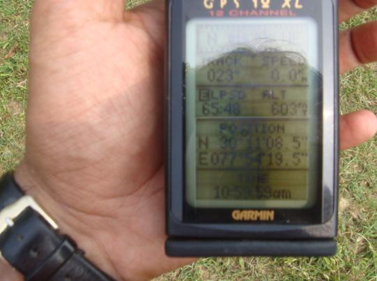
90 Piedmont open forest Siwalik hill forest Siwalik moderate forest Siwalik moderate forest Upper piedmont forest Siwalik hill 78

91 Appendix - 2 Laboratory analysis of soil samples - photographs (a) (b) (c) (d) Figure (a) soil samples and (Fig b, c, d) lab analysis of soil organic carbon. 79