Solutions 1-4 by Poya Khalaf

Transcription

1 Solutions -4 by Poya Khalaf. Consider the function: f { t < [ e t sin(t), te 2t] T t Calculate f 2,[, ] using the time-domain definition and then using Parsevals identity. The following code has been written to calculate the integrals using Matlab s symbolic toolbox: clc 2 clear 3 4 syms t w T 5 6 f=[exp(-t)*sin(t),t*exp(-2*t)].'; 7 8 %time domain definition 9 % int ˆinf [ f ˆ2dt disp('time domain definition') intf=int(f()ˆ2+f(2)ˆ2,t,,inf); 2 vpa(intf) 3 %frequency domain definition 4 %Fourier transform 5 F(,)=int(f().*exp(-i*w*t),t,,inf); 6 F(2,)=int(f(2).*exp(-i*w*t),t,,inf); 7 8 %int -infˆinf F*Fdw 9 intf=/(2*pi)*int(f'*f,w,-inf,inf); 2 disp('frequency domain definition') 2 vpa(intf,5) The results are as follows: time domain definition 2 ans = frequency domain definition 5 ans = Find an example of two LTI systems (to be cascaded) where the H 2 norm violates the submultiplicative property. Consider the two systems G = iω+ and H = 2 i ω+. The following code has been wriiten to calulate the 2-norm for the cascade system GH and G 2 H 2 : syms w 2 G=/(i*w+); 3 4 H=/(2*i*w+); 5 6 norm2gh=(/(2*pi)*int((g*h)'*(g*h),-inf,inf))ˆ.5; 7 disp(' GH ') 8 vpa(norm2gh,5) 9 norm2g=(/(2*pi)*int((g)'*(g),-inf,inf))ˆ.5; norm2h=(/(2*pi)*int((h)'*(h),-inf,inf))ˆ.5; 2 3 disp(' G * H ') 4 vpa(norm2g*norm2h,5)

2 The results are as follows: GH 2 ans = G * H 5 ans = It is seen that the 2-norm does not satisfy the submultiplicative property. Consider a system G(s) formed by cascading a pure time-shift operator S(s) and a first-order lag L(s): G(s) = L(s)S(s) S(s) = e bs L(s) = τs + Recall that the time-shift operator has the input-output relationship: u(t) u(t + b). When b <, this represents a delay, and b > corresponds to an advance. Pick your own value of τ. In this exercise, you will be illustrating the definition of causality in relation to G(s). a) Choose a value of b < and a truncation time T > to facilitate your example. Suppose the input to G(s) is a unit step. Use sketches of the signals at various points to Show that P T GP T u = P T Gu in this case. b) Now use a positive value of b with the same absolute value as above and the same T. Use sketches to show that P T GP T u P T Gu. c) The above proves (by counterexample) that G(s) is not causal if b >. For extra credit, prove mathematically that G is causal if and only if b <. a) For this purpose the following Matlab code has been written: s=tf('s'); 2 tau=.5; 3 T=3; 4 b=-; 5 6 L=/(tau*s+); 7 8 % Lu 9 [y,t]=step(l); t2=t; plot(t,y) 2 xlabel('time(s)') 3 ylabel('amplitude') 4 5 % Gu 6 t=t-b; 7 hold on 8 plot(t,y,'r') 9 title(['b=',num2str(b)]) 2 2 %P TGu 22 y(t>t)=; 23 hold on 24 plot(t,y,'k') 2

3 25 legend('lu','gu','p TGu') % P Tu 28 u=ones(length(t2),); 29 u(t2>t)=; 3 3 %GP Tu 32 [y2,t2]=lsim(l,u,t2); 33 t2=t2-b; 34 figure 35 plot(t2,y2) 36 xlabel('time(s)') 37 ylabel('amplitude') 38 title(['b=',num2str(b)]) 39 4 %P TGP Tu 4 y2(t2>t)=; 42 hold on 43 plot(t2,y2,'k') 44 legend('gp Tu','P TGP Tu') figure 48 plot(t,y,t2,y2) 49 legend('p TGu','P TGP Tu') 5 xlabel('time(s)') 5 ylabel('amplitude') 52 title(['b=',num2str(b)]) The results are as follows: b= Lu Gu P T Gu Amplitude time(s) 3

4 .9.8 b= GP T u P T GP T u.7 Amplitude time(s).9.8 b= P T Gu P T GP T u.7 Amplitude time(s) b) Using the above code for b = : 4

5 b= Lu Gu P T Gu Amplitude time(s).9.8 b= GP T u P T GP T u.7 Amplitude time(s) 5

6 .9.8 b= P T Gu P T GP T u.7 Amplitude time(s) c) Initially we find the expression for P T Gu. The transfer function L in the time domain is equal to: ẏ = τ y + τ u Also G = LS. In order to calculate GU we intially calculate SU. In the time domain SU is equal to: SU(t) = u(t + b) GU is found to be: Finally, P T GU is equal to: GU(t) = e t τ y + e t τ t e z τ u(z + b)dz Next, we calculate P T GP T U. P T U is equal to: { e t τ y P T GU(t) = + e t t τ e z τ u(z + b)dz t T t > T P T U(t) = { u t T t > T SP T U is found to be: GP T U is equal to: GP T U(t) = SP T U(t) = { { u(t + b) t T b t > T b e t τ y + e t t τ e z τ u(z + b)dz t T b e t τ y + e t T b τ e z τ u(z + b)dz t > T b 6

7 Now to calculate P T GP T U we consider two cases, b > and b <. In the first case if b > then T b < T and we have: e t τ y + e t t τ e z τ u(z + b)dz t T b P T GP T U(t) = e t τ y + e t T b τ e z τ u(z + b)dz T b < t < T t > T In this case we see that P T GP T U P T Gu. For the case b <, T b = T + b > T. Therefore P T GP T is found to be: { e t τ y P T GP T U(t) = + e t t τ e z τ u(z + b)dz t T t > T In this case we see that P T GP T U = P T Gu. Refer to the proof of the Small Gain Theorem in Green and Limebeer, Sect Provide full justification for the derivation of the inequality Se 2T Sê 2T 2,[,T ] γ(g )γ(g 2 ) e 2T ê 2T 2,[,T ] From the definition of Se 2T we have: Se 2T Sê 2T 2,[,T ] = G (w T + P T (G 2 e 2T )) G (w T + P T (G 2 ê 2T )) 2,[,T ] Since G has finite incremental gain we can write: G (w T + P T (G 2 e 2T )) G (w T + P T (G 2 ê 2T )) 2,[,T ] γ(g ) w T +P T (G 2 e 2T ) w T P T (G 2 ê 2T ) 2,[,T ] Which simplifies to: Se 2T Sê 2T 2,[,T ] γ(g ) P T (G 2 e 2T ) P T (G 2 ê 2T ) 2,[,T ] From the definition of the truncation operator we have: Since the norm is on [, T ] we can write: Se 2T Sê 2T 2,[,T ] γ(g ) P T (G 2 e 2T G 2 ê 2T ) 2,[,T ] Now since G 2 has finite incremental gain we have: Se 2T Sê 2T 2,[,T ] γ(g ) G 2 e 2T G 2 ê 2T 2,[,T ] Se 2T Sê 2T 2,[,T ] γ(g ) G 2 e 2T G 2 ê 2T 2,[,T ] γ(g )γ(g 2 ) e 2T ê 2T 2,[,T ] And therefore: Se 2T Sê 2T 2,[,T ] γ(g )γ(g 2 ) e 2T ê 2T 2,[,T ] 7

8

9

10

11

12

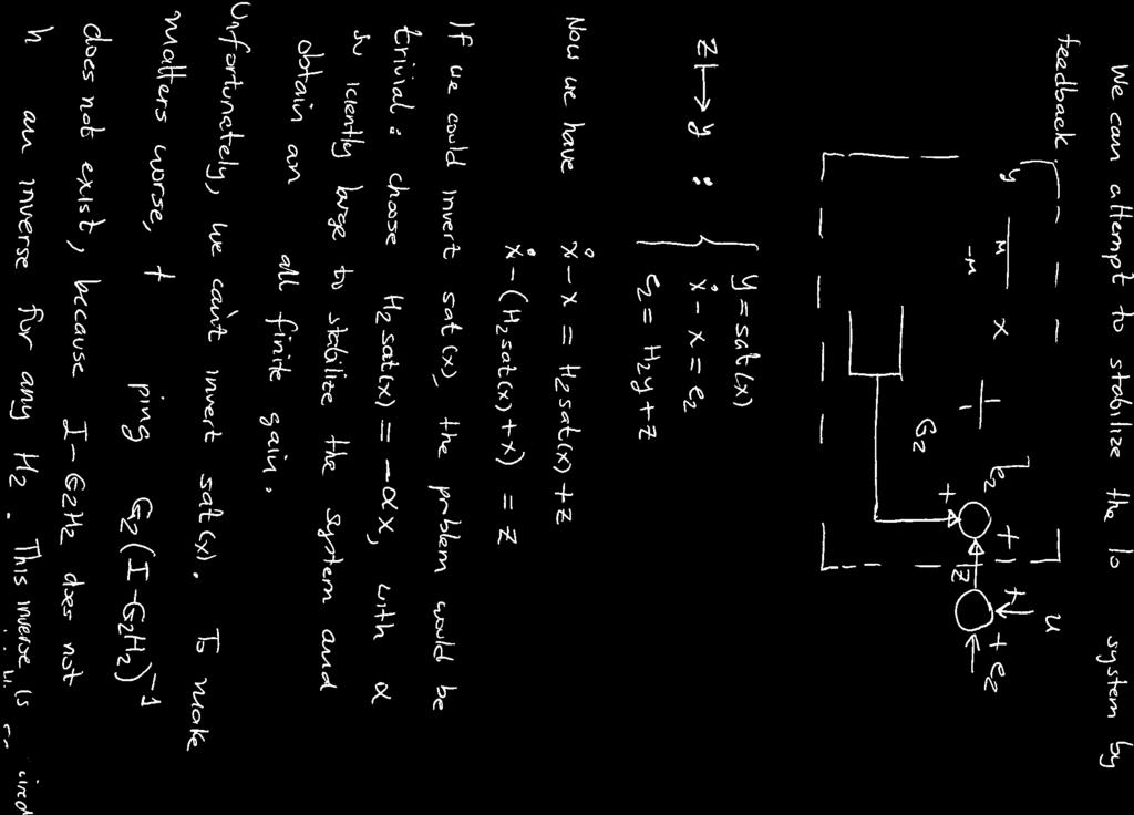
13 ESC794 Simulation Results: HWG The sliding mode controller was used first strictly as an output feedback controller (no feedback from signal x behind the saturation block). For all simulations λ was chosen as, and the switching gain η was chosen as. Figure shows the simulation diagram for this case. A saturation level M = was used first and the sign function in the controller was approximated using a saturation function applied to.s. The controller is able to arrest exponential growth of x and bring all internal signals to zero. The results are shown in Fig. 2. Note that the lower saturation block is active in several intervals. However,.s <, so the SMC is acting linearly. This is essentially a PI controller. Next, if M is reduced to.5, this controller is unable to stabilize x, as shown in Fig. 3. As a result, e and e 2 are not in L 2. Adding information about x as feedback will improve the controller, although this is no longer an output-based solution. As explained in the analysis, the term (λ+)x should be used in the control law. This is shown in the simulation diagram of Fig. 4. The controller is re-tuned to use s directly as the input to the saturation block. This time, M can be set to a value as low as. with internal stability. The results are shown in Fig. 5. A formal proof of stability would require advance knowledge of bounds on the external signals u and u 2, as well as the saturation level M.

14 s Step To Workspace7 s. Integrator Gain Gain3 Saturation Gain2 Pulse Generator Product WITHOUT x STATE FEEDBACK Gain u e To Workspace2 y To Workspace6 To Workspace3 x e2 To Workspace4 t To Workspace5 Clock To Workspace Saturation s Transfer Fcn Product u2 Pulse Generator To Workspace Figure : Simulation diagram of output-feedback SMC Results with saturation level M=, no X feedback 6 Signals x and y x y Sliding Function s e.5 e Time Time Figure 2: Results with output-feedback SMC and M =

15 5 Results with saturation level M=.5, no X feedback Signals x and y x y Sliding Function s e e Time Time Figure 3: Results with output-feedback SMC and M =.5 s Step To Workspace7 s Integrator Gain Gain3 Saturation Gain2 Pulse Generator Product WITH x STATE FEEDBACK Gain u e To Workspace2 y To Workspace6 To Workspace3 x e2 To Workspace4 t To Workspace5 Clock To Workspace Saturation s Transfer Fcn Product u2 Pulse Generator To Workspace Figure 4: Simulation diagram of SMC with x feedback

16 Signals x and y Results with saturation level M=. and X feedback 2 x y Sliding Function s e.4 e Time Time Figure 5: Results with x feedback SMC and M =.