Chapter 3 Convolution Representation

Size: px

Start display at page:

Download "Chapter 3 Convolution Representation"

Angelica Richards
5 years ago
Views:

1 Chapter 3 Convolution Representation

2 DT Unit-Impulse Response Consider the DT SISO system: xn [ ] System yn [ ] xn [ ] = δ[ n] If the input signal is and the system has no energy at n = 0, the output yn [ ] = hn [ ] is called the impulse response of the system δ[ n] System hn [ ]

3 Example Consider the DT system described by yn [ ] + ayn [ 1] = bxn [ ] Its impulse response can be found to be n ( a) b, n= 0,1,2, hn [ ] = 0, n = 1, 2, 3,

4 Representing Signals in Terms of Shifted and Scaled Impulses Let x[n] be an arbitrary input signal to a DT LTI system Suppose that for This signal can be represented as xn [ ] = x[0] δ[ n] + x[1] δ[ n 1] + x[2] δ[ n 2] + = = i= 0 xn [ ] = 0 n = 1, 2, xi [] δ[ n i], n 0,1,2,

5 Exploiting Time-Invariance and Linearity yn [ ] = xihn [ ] [ i], n 0 i= 0

6 The Convolution Sum This particular summation is called the convolution sum yn [ ] = xihn [ ] [ i] i= 0 xn [ ] hn [ ] yn [ ] = xn [ ] hn [ ] Equation is called the convolution representation of the system Remark: a DT LTI system is completely described by its impulse response h[n]

7 Block Diagram Representation of DT LTI Systems Since the impulse response h[n] provides the complete description of a DT LTI system, we write xn [ ] hn [ ] yn [ ]

8 The Convolution Sum for Noncausal Signals Suppose that we have two signals x[n] and v[n] that are not zero for negative times (noncausal signals) Then, their convolution is expressed by the two-sided series yn [ ] = xivn [ ] [ i] i=

9 Example: Convolution of Two Rectangular Pulses Suppose that both x[n] and v[n] are equal to the rectangular pulse p[n] (causal signal) depicted below

10 The Folded Pulse v[ i] The signal is equal to the pulse p[i] folded about the vertical axis

11 vn [ i ] xi [] Sliding over

12 vn [ i ] xi [] Sliding over - Cont d

13 Plot of xn [ ] vn [ ] Plot of

14 Properties of the Convolution Sum Associativity xn [ ] ( vn [ ] wn [ ]) = ( xn [ ] vn [ ]) wn [ ] Commutativity xn [ ] vn [ ] = vn [ ] xn [ ] Distributivity w.r.t. addition xn [ ] ( vn [ ] + wn [ ]) = xn [ ] vn [ ] + xn [ ] wn [ ]

15 Properties of the Convolution Sum - Cont d x [ q n ] = x [ n q ] v [ q n ] = v [ n q ] wn [ ] = xn [ ] vn [ ] w[ n q] = x [ n] v[ n] = x[ n] v [ n] Shift property: define then q Convolution with the unit impulse xn [ ] δ[ n] = xn [ ] Convolution with the shifted unit impulse xn [ ] δ [ n] = xn [ q] q q

16 Example: Computing Convolution with Matlab Consider the DT LTI system xn [ ] hn [ ] yn [ ] impulse response: input signal: hn [ ] = sin(0.5 n), n 0 xn [ ] = sin(0.2 n), n 0

17 Example: Computing Convolution with Matlab Cont d hn [ ] = sin(0.5 n), n 0 xn [ ] = sin(0.2 n), n 0

18 Example: Computing Convolution with Matlab Cont d Suppose we want to compute y[n] for n = 0,1,,40 Matlab code: n=0:40; x=sin(0.2*n); h=sin(0.5*n); y=conv(x,h); stem(n,y(1:length(n)))

19 Example: Computing Convolution with Matlab Cont d yn [ ] = xn [ ] hn [ ]

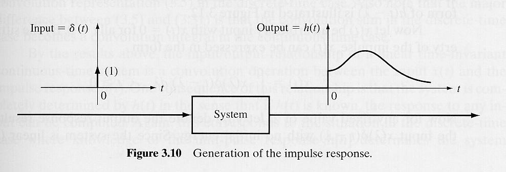
20 CT Unit-Impulse Response Consider the CT SISO system: xt () System yt () xt () = δ () t If the input signal is and the system has no energy at t = 0, the output yt () = ht () is called the impulse response of the system δ () t System ht ()

21 Exploiting Time-Invariance Let x[n] be an arbitrary input signal with xt () = 0, for t< 0 Using the sifting property of δ () t, we may write xt () = x( τδ ) ( t τ) dτ, t 0 0 Exploiting time-invariance invariance, it is δ ( t τ ) System ht ( τ )

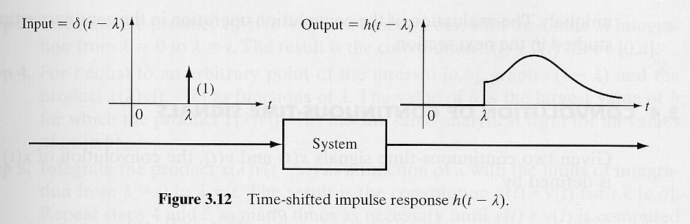
22 Exploiting Time-Invariance

23 Exploiting Linearity Exploiting linearity, it is yt () = x( τ) ht ( τ) dτ, t 0 0 x( ) h( t ) If the integrand τ τ does not contain an impulse located at τ = 0, the lower limit of the integral can be taken to be 0,i.e., yt () = x( τ) ht ( τ) dτ, t 0 0

24 The Convolution Integral This particular integration is called the convolution integral yt () = x( τ) ht ( τ) dτ, t 0 0 xt () ht () yt () = xt () ht () Equation is called the convolution representation of the system Remark: a CT LTI system is completely described by its impulse response h(t)

25 Block Diagram Representation of CT LTI Systems Since the impulse response h(t) provides the complete description of a CT LTI system, we write xt () ht () yt ()

26 Example: Analytical Computation of the Convolution Integral xt () = ht () = pt (), Suppose that where p(t) is the rectangular pulse depicted in figure pt () 0 T t

27 Example Cont d In order to compute the convolution integral yt () = x( τ) ht ( τ) dτ, t 0 0 we have to consider four cases:

28 Case 1: t 0 Example Cont d ht ( τ ) x( τ ) t T t 0 T τ yt () = 0

29 Case 2:0 t T Example Cont d ht ( τ ) x( τ ) t T 0 t T τ t yt () = dτ = t 0

30 Example Cont d Case 3: 0 t T T T t 2T x( τ ) ht ( τ ) 0 t T T t τ T yt () = dτ = T ( t T) = 2T t t T

31 Example Cont d Case 4: T t T 2T t x( τ ) ht ( τ ) 0 T t T t τ yt () = 0

32 Example Cont d yt () = xt () ht () T 0 t 2T

33 Properties of the Convolution Integral Associativity xt () ( vt () wt ()) = ( xt () vt ()) wt () Commutativity xt () vt () = vt () xt () Distributivity w.r.t. addition xt () ( vt () + wt ()) = xt () vt () + xt () wt ()

34 Properties of the Convolution Integral - Cont d x () q t = x ( t q ) v () q t = v ( t q ) wt () = xt () vt () w( t q) = x () t v() t = x() t v () t Shift property: define then Convolution with the unit impulse q xt () δ () t = xt () Convolution with the shifted unit impulse xt () δ () t = xt ( q) q q

35 Properties of the Convolution Integral - Cont d Derivative property: if the signal x(t) is differentiable, then it is d dt dx() t xt () vt () = vt () dt [ ] If both x(t) and v(t) are differentiable, then it is also d 2 [ xt () vt ()] = dx t dv t 2 () () dt dt dt

36 Properties of the Convolution Integral - Cont d Integration property: define t then ( 1) x () t x( τ ) d t ( 1) v () t v( ) d ( 1) ( 1) ( 1) ( x v) () t = x () t v() t = x() t v () t τ τ τ

37 Representation of a CT LTI System in Terms of the Unit-Step Response Let g(t) be the response of a system with impulse response h(t) when xt () = ut () with no initial energy at time, i.e., t = 0 ut () ht () gt () Therefore, it is gt () = ht () ut ()

38 Representation of a CT LTI System in Terms of the Unit-Step Response Cont d Differentiating both sides Recalling that it is dg () t () () = dh t ut () = ht () du t dt dt dt du() t dt dg() t dt = δ () t and ht () = ht () δ () t = ht () or t gt () = h( τ ) dτ 0

06/12/ rws/jMc- modif SuFY10 (MPF) - Textbook Section IX 1

06/12/ rws/jMc- modif SuFY10 (MPF) - Textbook Section IX 1 IV. Continuous-Time Signals & LTI Systems [p. 3] Analog signal definition [p. 4] Periodic signal [p. 5] One-sided signal [p. 6] Finite length signal [p. 7] Impulse function [p. 9] Sampling property [p.11]