DSP Algorithm Original PowerPoint slides prepared by S. K. Mitra
|
|
|
- Mary Smith
- 6 years ago
- Views:
Transcription
1 Chapter 11 DSP Algorithm Implementations 清大電機系林嘉文 Original PowerPoint slides prepared by S. K. Mitra
2 Matrix Representation of Digital Consider Filter Structures This structure is described by the set of equations w 1 1[ [n] = x[n] [ ] α w 5 5[ [n] w 2 [n] =w 1 [n] δ w 3 [n] w 3 [n] = w 2 [n 1] w 4 [n] = w 3 [n] + ε w 2 [n] w 5 [n] = w 4 [n 1] y[n] =ββ w 1 [n] + γ w 5 [n] Original PowerPoint slides prepared by S. K. Mitra 11-2
3 Matrix Representation of Digital Filter Structures This ordered ed set of equations is said to be noncomputable because some variables on the left side are computed before some right-side variables are made available For example, computation of w 1 [n] in the 1st step requires the knowledge of w 5 [n] which is computed in the 5th step Likewise, computation of w 2 [n] in the 2nd step requires the knowledge of w 3 [n] that is computed in the 3rd step Suppose we reorder the equations w 3 [n] = w 2 [n 1] w 5 [n] = w 4 [n 1] w 1 [n] = x[n] α w 5 [n] w 2 [n] =w 1 [n] δ w 3 [n] w 4 [n] =w w 3 [n] +εε w 2 [n] y[n] = β w 1 [n] + γ w 5 [n] Original PowerPoint slides prepared by S. K. Mitra 11-3


4 Matrix Representation This new ordered ed set of equations is computable In most practical applications, equations describing a digital filter structure can be put into a computable order by inspection A simple way to examine the computability of equations describing a digital filter structure is by writing the equations in a matrix form A matrix representation of the first ordered set of equations: Original PowerPoint slides prepared by S. K. Mitra 11-4
![Matrix Representation In compact form y[n] = x[n] + F y[n] + G y[n 1] where y[n] = [w 1 [n] w 2 [n] w 3 [n] w 4 [n] w 5 [n] y[n]] T x[n] = [x[n] 0 0 0 0 0] T If a diagonal element of F is nonzero,](/docs-images/75/72666747/images/5-0.jpg "then computation of present value of the corresponding variable requires the knowledge of its present value implying py presence of a delay-free loop Original PowerPoint slides prepared by S. K.")
5 Matrix Representation In compact form y[n] = x[n] + F y[n] + G y[n 1] where y[n] = [w 1 [n] w 2 [n] w 3 [n] w 4 [n] w 5 [n] y[n]] T x[n] = [x[n] ] T If a diagonal element of F is nonzero, then computation of present value of the corresponding variable requires the knowledge of its present value implying py presence of a delay-free loop Original PowerPoint slides prepared by S. K. Mitra 11-5
6 Matrix Representation Any nonzero o entries es in the same row above the main diagonal of F imply that the computation of present value of the corresponding variable requires present values of other variables not yet computed, making the set of equations noncomputable Hence, for computability all elements of F matrix on the diagonal and above diagonal must be zeros In the F matrix for the first ordered set of equations, diagonal elements are all zeros, indicating absence of delay-free loops However, there are nonzero entries above the diagonal in the first and second rows of F indicating that the set of equations are not in proper order for computation Original PowerPoint slides prepared by S. K. Mitra 11-6

7 Matrix Representation The F matrix for the second ordered ed set of equations is which is seen to satisfy the computability condition Original PowerPoint slides prepared by S. K. Mitra 11-7
8 Precedence Graph The precedence graph can be used to test the computability of a digital filter structure and to develop the proper ordering sequence for a set of equations describing a computable structure It is developed from the signal-flow graph description of the digital filter structure in which independent and dependent signal variables are represented by nodes, and the multiplier and delay branches are represented by directed d branches The directed branch has an attached symbol denoting the branch gain or transmittance For a multiplier branch, the branch gain is the multiplier coefficient value For a delay branch, the branch gain is simply z 1 Original PowerPoint slides prepared by S. K. Mitra 11-8
9 Precedence Graph The signal-flow graph representation of is shown below Original PowerPoint slides prepared by S. K. Mitra 11-9
10 Precedence Graph A reduced signal-flow graph is then developed by removing the delay branches and all branches going out of the input node The reduced signal-flow graph of the example digital filter structure is shown below Original PowerPoint slides prepared by S. K. Mitra 11-10
11 Precedence Graph The nodes in the reduced signal-flow graph are grouped as follows: All nodes with only outgoing branches are grouped into one set labeled {N 1 } Next, the set {N 2 } is formed containing nodes coming in only from one or more nodes in the set {N 1 1} and have outgoing branches to the other nodes Then, form the set {N 3 } containing nodes that have branches coming in only from one or more nodes in the sets {N 1 } and {N 2 }, and have outgoing branches to other nodes Continue the process until there is a set of nodes {N f } containing only incoming branches The rearranged graph is called a precedence graph Original PowerPoint slides prepared by S. K. Mitra 11-11
12 Precedence Graph Since signal variables belonging to {N 1 } do not depend on the present values of other signal variables, these variables should be computed first Next, signal variables belonging to {N 2 } can be computed since they depend on the present values of signal variables contained in {N 1 1} that have already been computed This is followed by the computation of signal variables in {N 3 }, {N 4 }, etc. Finally, in the last step the signal variables in {N f } are computed This process of sequential computation ensures the development of a valid computational algorithm If there is no final set {N f f} } containing only incoming branches, the digital filter structure is noncomputable Original PowerPoint slides prepared by S. K. Mitra 11-12
13 Precedence Graph For the example precedence graph, pertinent groupings of node variables are: {N 1 } = {w 3 [n], w 5 [n]} {N 2 }={w 1 [n]} {N 3 } = {w 2 [n]} {N 4 4} = {w 4 4[ [n], y[n]} Original PowerPoint slides prepared by S. K. Mitra 11-13
14 Precedence Graph Precedence graph redrawn according to the above groupings is as shown below Since the final node set {N 4 } has only incoming branches, the structure is computable Original PowerPoint slides prepared by S. K. Mitra 11-14
15 Structure Verification A simple method to verify that the structure developed is indeed characterized by the prescribed transfer function H(z) Consider for simplicity a causal 3rd order IIR transfer function If {h[n]} denotes its impulse response, then Note P(z) = H(z)D(z), which is equivalent to Original PowerPoint slides prepared by S. K. Mitra 11-15
![Structure Verification Evaluate above convolution sum for 0 n 6: p 0 = h[0] p 1 = h[1] + h[0]d 1 p 2 =h[2] +h[1]d 1 +h[0]d 2 p 3 = h[3] + h[2]d 1 + h[1]d 2 + h[0]d 3 0 = h[4] [ ] +](/docs-images/75/72666747/images/16-0.jpg "h[3]d[ ] 1 + h[2]d[ ] 2 + h[1]d[ ] 3 0 = h[5] + h[4]d 1 + h[3]d 2 + h[2]d 3 0 = h[6] + h[5]d 1 + h[4]d 2 + h[3]d 3 In matrix form we get Original PowerPoint slides prepared by S. K.")
16 Structure Verification Evaluate above convolution sum for 0 n 6: p 0 = h[0] p 1 = h[1] + h[0]d 1 p 2 =h[2] +h[1]d 1 +h[0]d 2 p 3 = h[3] + h[2]d 1 + h[1]d 2 + h[0]d 3 0 = h[4] [ ] + h[3]d[ ] 1 + h[2]d[ ] 2 + h[1]d[ ] 3 0 = h[5] + h[4]d 1 + h[3]d 2 + h[2]d 3 0 = h[6] + h[5]d 1 + h[4]d 2 + h[3]d 3 In matrix form we get Original PowerPoint slides prepared by S. K. Mitra 11-16

17 Structure Verification In partitioned form above matrix equation can be written as Where Solving second equation we get Substituting above in the first equation we get In the case of an N-th order IIR filter, the coefficients of its transfer function can be determined from the first 2N+1 impulse response samples Original PowerPoint slides prepared by S. K. Mitra 11-17
![Structure Verification Example: Consider the causal transfer function Here Hence h[0] = 2, h[1] = 4, h[2]](/docs-images/75/72666747/images/18-0.jpg "= 5, h[3] = 3, h[4] =13 Solving the above we get Original PowerPoint slides prepared by S. K. Mitra 11-18")
18 Structure Verification Example: Consider the causal transfer function Here Hence h[0] = 2, h[1] = 4, h[2] = 5, h[3] = 3, h[4] =13 Solving the above we get Original PowerPoint slides prepared by S. K. Mitra 11-18
19 Four Classes of Fourier Transforms Continuous in Time Discrete in time-periodic in frequency FT DTFT; T 0 f(k) F(e jωt 0 ) in Con ntinuous freq uency f F t k ω 1 jω t T0 ( t ) = F ( jω ) e dω ( k) = 2π 2π jω t = f ( t e dt ( ω ) ) π T0 f π T 0 F ( e jωt 0 ) jωt jk T F e 0 = f k ) ω 0 ( ) ( e k = e jkωt 0 2π T 0 dω Fourier transform Discrete time Fourier Transform Original PowerPoint slides prepared by S. K. Mitra 11-19
20 Four Classes of Fourier Transforms Continuous in Time Discrete in time-periodic in frequency period dic in quency Discre ete in fre time 2π ω 0 f ( t) F F(n) f(t) F(k) F(n) t nω 0 k n FS i ω 0 DFT:N N jnω t F ( n) e 1 2π 1 j kn N f ( k) = F( n) e n= N n= 0 = 0 ω 2π π 0 ω0 ( n) = π ω 0 f ( t) e jnω t 0 dt F( n) = N 1 2π j kn N f ( k) e k = 0 Fourier series Discrete Fourier Transform Original PowerPoint slides prepared by S. K. Mitra 11-20
21 Direct Computation of DFT For a complex-valued sequence of N C C DFT SUBROUTINE points the DFT may be expressed as C ISEL = 0 : DFT C ISEL = 1 : INVERSE DFT N C 1 2πkn 2πkn X R ( k) = xr ( n)cos + xi ( n)sin SUBROUTINE DFT(N, XR, XI, XFR, XFI, ISEL) n= 0 N N DIMENSION XR(N), XI(N), XFR(N), XFI(N) N WN = / FLOAT(N) 1 2πkn 2πkn X I ( k) = xr ( n)sin xi ( n)cos IF (ISEL.EQ.1) WN = - WN n= 0 N N DO 20 K = 1, N XFR(K) = 0, The direct computation XFI(K) = 0, KM1 = K 1 requires: DO 20 I = 1, N 2N 2 IM1 = I 1 evaluations of trigonometric ARG = WN * KM1 * IM1 C = COS(ARG) functions. S = SIN(ARG) 4N 2 XFR(K) = XFR(K) + XR(I)*C + XI(I)*S real multiplications. XFI(K) = XFI(K) XR(I)*S + XI(I)*C 10 CONTINUE 4N(N 1 ) real additions. IF (ISEL 1) 20, 30, XFR(K) = XFR(K) / FLOAT(N) A number of indexing and 20 XFI(K) = XFI(K) / FLOAT(N) addressing operations. CONTINUE RETURN END Original PowerPoint slides prepared by S. K. Mitra 11-21

22 Goertzel s Algorithm A recursive DFT computation scheme that makes use of the identity obtained using the periodicity of Using this identity we can write Original PowerPoint slides prepared by S. K. Mitra 11-22


23 Define Goertzel s Algorithm Note: y k [n] is the direct convolution of the causal sequence with a causal sequence Observe X[k] = y k [n] n=n z-transform of yields Original PowerPoint slides prepared by S. K. Mitra 11-23
24 Goertzel s Algorithm Thus, y k [n] is the output of an initially relaxed LTI digital filter H k [z] with an input x e [n] and, when n = N, y k [n] = X[k] Structural interpretation of the algorithm Thus a recursive DFT computation scheme is with y k [ 1] = 0 and x e [N] = 0 Original PowerPoint slides prepared by S. K. Mitra 11-24
25 Goertzel s Algorithm Since a complex multiplication needs 4 real multiplications and 2 real additions, computation of each new value of y k [n] requires 4 real multiplications and 4 real additions Thus computation of X[k] = y k [N] involves 4N real multiplications and 4N real additions Computation ti of all N DFT samples requires 4N 2 real multiplications and 4N 2 real additions Direct computation of all N samples of {X[k]} requires N 2 complex multiplications and N(N-1) complex additions Equivalently, direct computation of all N samples of {X[k]} requires 4N 2 real multiplications and N(4N-2) real additions Thus, Goertzel s algorithm requires 2N more real additions than the direct DFT computation Original PowerPoint slides prepared by S. K. Mitra
![Goertzel s Algorithm The algorithm can be made computationally more efficient by observing that H k [z] can](/docs-images/75/72666747/images/26-0.jpg "be rewritten as resulting in a second-order realization Original PowerPoint slides prepared by S. K.")
26 Goertzel s Algorithm The algorithm can be made computationally more efficient by observing that H k [z] can be rewritten as resulting in a second-order realization Original PowerPoint slides prepared by S. K. Mitra 11-26
27 Goertzel s Algorithm DFT computation equations are now Computation of each sample of involves only 2 real multiplications and 4 real additions Complex multiplication by needs to be performed only once at n = N Thus, computation of one sample of X[k] requires (2N+4) real multiplications and (4N+4) real additions Computation of all N DFT samples requires 2N(N+2) real multiplications and 4N(N+1) real additions Original PowerPoint slides prepared by S. K. Mitra 11-27
28 Goertzel s Algorithm In realizing H N k [z], the multiplier in the feedback path is 2cos(2π(N k)/n) = 2cos(2πk/N) which is same as that in the realization of H k k[ [z] ν N k [n] = ν k [n], i.e., the intermediate variables computed to determine X[k] can again be used to determine X[N k] Only difference between the two structures is the feedforward multiplier which is now that is the complex conjugate of Thus, computation of X[k] and X[N k] require 2(N+4) real multiplications and 4(N+2) real additions Computation of all N DFT samples require approximately N 2 real multiplications and approximately 2N 2 real additions Original PowerPoint slides prepared by S. K. Mitra 11-28
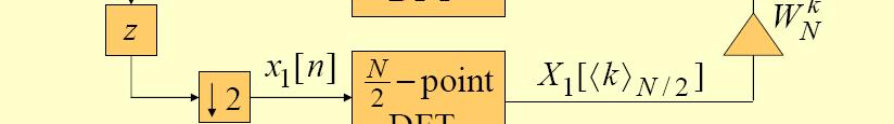
![Decimation-in-Time in FFT Algorithm Consider a sequence x[n] of length N = 2 μ Using a 2-band polyphase decomposition we can express its z-transform as where X(z) ) = X 1 0 (z 2 ) + z 1 X 1 (z 2 )](/docs-images/75/72666747/images/29-0.jpg "Evaluating on the unit circle at N equally spaced points we arrive at the N-point p DFT of x[n]: [ ] where X 0 0[ [k] and X 1 1[ [k] are the (N/2)-point DFTs of x 0 0[ [n] and x 1 [n] 11-29 Original")
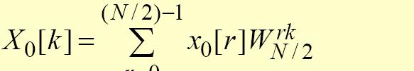
29 Decimation-in-Time in FFT Algorithm Consider a sequence x[n] of length N = 2 μ Using a 2-band polyphase decomposition we can express its z-transform as where X(z) ) = X 1 0 (z 2 ) + z 1 X 1 (z 2 ) Evaluating on the unit circle at N equally spaced points we arrive at the N-point p DFT of x[n]: [ ] where X 0 0[ [k] and X 1 1[ [k] are the (N/2)-point DFTs of x 0 0[ [n] and x 1 [n] Original PowerPoint slides prepared by S. K. Mitra
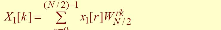
30 Decimation-in-Time in FFT Algorithm That is Block diagram interpretation: Original PowerPoint slides prepared by S. K. Mitra 11-30
31 Decimation-in-Time in FFT Algorithm Flow-graph representation Original PowerPoint slides prepared by S. K. Mitra 11-31
32 Decimation-in-Time in FFT Algorithm Direct computation of the N-point DFT requires N 2 complex multiplications and N 2 N N 2 complex additions The modified scheme requires the computation of two (N/2)-point DFTs that are then combined with N complex multiplications and N complex additions resulting in a total of (N 2 /2) + N complex multiplications and approximately (N 2 /2) + N complex additions For N 3,, (N 2 /2)) + N < N 2 Original PowerPoint slides prepared by S. K. Mitra 11-32
33 Decimation-in-Time in FFT Algorithm Continuing the process we can express and as a weighted combination of two (N/4)-point DFTs For example, we can write where X 00 [k] and X 01 [k] are the (N/4)-point DFTs of the (N/4)-length sequences x 00 [n] = x 0 [2n] and x 01 [n] = x 0 [2n+1] Likewise, we can express where X 10 [k] and X 11 [k] are the (N/4)-point DFTs of the (N/4)-length sequences x 10 [n] = x 1 [2n] and x 11 [n] = x 1 [2n+1] Original PowerPoint slides prepared by S. K. Mitra 11-33
34 Decimation-in-Time in FFT Algorithm Block-diagram representation of the two-stage algorithm Original PowerPoint slides prepared by S. K. Mitra 11-34
35 Decimation-in-Time in FFT Algorithm Flow-graph representation Original PowerPoint slides prepared by S. K. Mitra 11-35
36 Decimation-in-Time in FFT Algorithm In the flow-graph shown N = 8 Hence, the (N/4)-point DFT here is a 2-point DFT and no further decomposition is possible The four 2-point DFTs, X ij [k], i, j = 0,1 can be easily computed For example Corresponding flow-graph of the 2-point DFT is shown below obtained using the identity Original PowerPoint slides prepared by S. K. Mitra 11-36
37 Decimation-in-Time in FFT Algorithm Complete flow-graph of the 8-point DFT is shown below Original PowerPoint slides prepared by S. K. Mitra 11-37
38 Decimation-in-Time in FFT Algorithm The flow-graph consists of 3 stages First stage computes the four 2-point DFTs Second stage computes the two 4-point DFTs Last stage computes the desired 8-point DFT The number of complex multiplications and additions at each stage is equal to 8, the size of the DFT Total number of complex multiplications and additions to compute all 8 DFT samples is equal to = 24 = 8 3 In the general case when N = 2 μ, the number of stages for computing the N-point DFT in the algorithm will be μ =logn 2 N Total number of complex multiplications and additions to compute all N DFT samples is N(log 2 N) Original PowerPoint slides prepared by S. K. Mitra 11-38
39 Decimation-in-Time in FFT Algorithm Note, and Besides, the coefficients have the symmetry property of These properties can be exploited to reduce the computational complexity further In the following basic module two output variables are generated by a weighted combination of two input variables The basic computational module is called a butterfly computation ti Original PowerPoint slides prepared by S. K. Mitra 11-39

40 Decimation-in-Time in FFT Algorithm The input-output relations of the basic module are: Substituting in the second equation given above we get The modified butterfly computation requires only one complex multiplication as indicated below Use of the above modified butterfly computation module reduces the total number of complex multiplications by 50% Original PowerPoint slides prepared by S. K. Mitra 11-40
41 Decimation-in-Time in FFT Algorithm New flow-graph using the modified butterfly computational module for N = 8 Original PowerPoint slides prepared by S. K. Mitra 11-41
42 Decimation-in-Time in FFT Algorithm Computational complexity can be reduced further by avoiding multiplications by,,, and The DFT computation algorithm described here also is efficient with regard to memory requirements Note: Each stage employs the same butterfly computation ti to compute Ψ r+1 [α] and Ψ r+1 [β] from Ψ r [α] and Ψ r [β] At the end of computation at any stage, output variables Ψ r+1 [m] can be stored in the same registers previously occupied by the corresponding input variables Ψ r [m] This type of memory location sharing is called in-place computation resulting in significant savings in overall memory requirements Original PowerPoint slides prepared by S. K. Mitra 11-42
43 Decimation-in-Time in FFT Algorithm In the DFT computation scheme outlined, the DFT samples X[k] appear at the output in a sequential order while the input samples x[n] appear in a different order Thus, a sequentially entiall ordered input x[n] must be reordered appropriately before the fast algorithm described by this structure can be implemented Original PowerPoint slides prepared by S. K. Mitra 11-43
44 Decimation-in-Time in FFT Algorithm To understand the input reordering scheme, represent the arguments of input samples x[n] and their sequentially ordered new representations Ψ 1 [m] in binary forms with the relations between the arguments m and n as follows: Thus, if (b 2 b 1 b 0 ) represents the index n of x[n], [ ] then the sample x[b 2 b 1 b 0 ] appears at the location m = b 0 b 1 b 2 as Ψ 1 [b 0 b 1 b 2 ] before the DFT computation is started i.e., the location of Ψ 1 [m] is in bit-reversed order from that of x[n] Alternative forms can be obtained by reordering the computations such as input in normal order and output in bitreversed order, and both input and output in normal order Original PowerPoint slides prepared by S. K. Mitra 11-44
45 Decimation-in-Time in FFT Algorithm The fast algorithm described assumes that the length of x[n] is a power of 2 If it is not, the length can be extended by zero-padding and make the length a power of 2 Even after zero-padding, the DFT computation based on the fast algorithm may be computationally more efficient than a direct DFT computation of the original shorter sequence The fast DFT computation schemes described are called decimation-in-time (DIT) fast Fourier transform (FFT) algorithms as input x[n] is first decimated to form a set of subsequences before the DFT is computed Original PowerPoint slides prepared by S. K. Mitra 11-45
46 Decimation-in-Time in FFT Algorithm For N = 2 μ, this decimation can be performed μ = log 2 N times. The total number of Complex multiplications : (N/2) log 2 N Complex additions : N log 2 N N Complex multiplications in Direct Computation N 2 Complex multiplications in FFT algorithm, (N/2)log 2 N , , , ,535 1, ,144 2,304 1,024 1,048,576 5,120 Original PowerPoint slides prepared by S. K. Mitra 11-46
47 Decimation-in-Time in FFT Algorithm For example, the relation between x[n] and its even and odd parts, x 0 [n] and x 1 [n], generated by the first stage of the DIT algorithm is given by Likewise, the relation between x[n] and the sequences x 00 [n], x 01 [n], x 10 [n], and x 11 [n], generated by the two-stage decomposition of the DIT algorithm is given by Original PowerPoint slides prepared by S. K. Mitra 11-47
48 Decimation-in-Time in FFT Algorithm The subsequences x 00 [n], x 01 [n], x 10 [n], and x 11 [n] can be generated directly by a factor-of-4 decimation process leading to a single-stage decomposition as shown below: Original PowerPoint slides prepared by S. K. Mitra 11-48
![Radix-RR FFT Algorithm Radix-R FFT algorithm - A each stage the decimation is by a factor of R Depending on N, various combinations of decompositions of X[k] can be used to develop elop different](/docs-images/75/72666747/images/49-0.jpg "types of DIT FFT algorithms If the scheme uses a mixture of decimations by different factors, it is called a mixed radix FFT algorithm For N which is a composite number expressible in the form of a")
49 Radix-RR FFT Algorithm Radix-R FFT algorithm - A each stage the decimation is by a factor of R Depending on N, various combinations of decompositions of X[k] can be used to develop elop different types of DIT FFT algorithms If the scheme uses a mixture of decimations by different factors, it is called a mixed radix FFT algorithm For N which is a composite number expressible in the form of a product of integers: N = r 1 r 2 r ν the total number of complex multiplications (additions) in a DIT FFT algorithm based on a ν -stage decomposition is given by Original PowerPoint slides prepared by S. K. Mitra 11-49


50 Decimation-in-Frequency in FFT Algorithm For k even For k odd We can write where Original PowerPoint slides prepared by S. K. Mitra 11-50
51 Decimation-in-Frequency in FFT Algorithm Thus X[2l] and X[2l+1] are the (N/2)-point DFTs of the length-(n/2) sequences x 0 [n] and x 1 [n], The flow-graph of the first-stage of the DFT: The output DFT samples appear in a decimated form with the even-indexed samples appearing as the output of one (N/2)-point DFT and the odd-indexed samples appearing as the output of the other (N/2)-point DFT Original PowerPoint slides prepared by S. K. Mitra
-point DFTs as a sum of two (N/4)- point DFTs The process is")
 FFT computation scheme for N = 8 Original PowerPoint slides")
52 Decimation-in-Frequency in FFT Algorithm We next express the even- and odd-indexed samples of each one of the two (N/2)-point DFTs as a sum of two (N/4)- point DFTs The process is continued until the smallest DFTs are 2-point DFTs The flow-graph of the decimation-in-frequency in (DIF) FFT computation scheme for N = 8 Original PowerPoint slides prepared by S. K. Mitra 11-52
53 Decimation-in-Frequency in FFT Algorithm Computational complexity of the radix-2 DIF FFT algorithm is same as that of the DIT FFT algorithm Various forms of DIF FFT algorithm can similarly be developed eloped The DIT and DIF FFT algorithms described here are often referred to as the Cooley-Tukey FFT algorithms Original PowerPoint slides prepared by S. K. Mitra 11-53
 Consider a length-n sequence x[n] with an N-point")
![DFT X[k] Recall Multiplying both sides by N and taking the complex conjugate we get Right-hand](/docs-images/75/72666747/images/54-1.jpg "side of above is the N-point DFT of a sequence X*[k] Original PowerPoint slides prepared by S. K.")
54 Inverse DFT Computation An FFT algorithm for computing the DFT samples can also be used to calculate efficiently the inverse DFT (IDFT) Consider a length-n sequence x[n] with an N-point DFT X[k] Recall Multiplying both sides by N and taking the complex conjugate we get Right-hand side of above is the N-point DFT of a sequence X*[k] Original PowerPoint slides prepared by S. K. Mitra 11-54


55 Inverse DFT Computation The desired IDFT x[n] is then obtained as Inverse DFT computation is shown below: Original PowerPoint slides prepared by S. K. Mitra 11-55

![DFT X[k] where N = N 1 N 2 Represent](/docs-images/75/72666747/images/56-1.jpg "the indices n and k as Using these")

56 Cooley-Tukey FFT Algorithms Consider a length-n sequence x[n] with an N-point DFT X[k] where N = N 1 N 2 Represent the indices n and k as Using these index mappings we can write as Original PowerPoint slides prepared by S. K. Mitra 11-56
57 Cooley-Tukey FFT Algorithms Since,, and, we have where 0 k 1 N 1 1 and 0 k 2 N 2 1 The effect of the index mapping is to map the 1-D sequence x[n] into a 2-D sequence that can be represented as a 2-D array with n 1 specifying the rows and n 2 specifying the columns of the array Inner parentheses of the last equation is seen to be the set of N 1 -point DFTs of the N 2 -columns: Original PowerPoint slides prepared by S. K. Mitra 11-57
58 Cooley-Tukey FFT Algorithms Note: The column DFTs can be done in place Next, these row DFTs are multiplied in place by the twiddle factors yielding Finally, the outer sum is the set of N 2-point DFTs of the columns of the array: The row DFTs, X[k 1 +N 1 k 1 ], can again be computed in place The input x[n] is entered into an array according to the index map: Original PowerPoint slides prepared by S. K. Mitra 11-58
59 Cooley-Tukey FFT Algorithms Likewise, the output DFT samples X[k] need to extracted from the array according to the index map: Example: Let N = 8. Choose N 1 = 2 and N 2 = 4, then for 0 k 1 1 and 0 k D array representation of the input is Original PowerPoint slides prepared by S. K. Mitra 11-59

60 Cooley-Tukey FFT Algorithms The column DFTs are 2-point DFTs given by These DFTs require no multiplications 2-D array of row transforms is After multiplying by the twiddle factors array becomes Original PowerPoint slides prepared by S. K. Mitra 11-60

61 Note Cooley-Tukey FFT Algorithms Finally, the 4-point DFTs of the rows are computed: Output 2-D array is given by The process illustrated is precisely the first stage of the DIF FFT algorithm Original PowerPoint slides prepared by S. K. Mitra 11-61

62 Cooley-Tukey FFT Algorithms By choosing N 1 = 4 and N 2 = 2, we get the first stage of the DIT FFT algorithm Alternate index mappings are given by Original PowerPoint slides prepared by S. K. Mitra 11-62


63 Prime Factor Algorithms Twiddle factors can be eliminated by defining the index mappings as To eliminate the twiddle factors we need to express Now It follows from above that if AC N = N 2, BD N = N 1, AD N = BC N = 0 then Original PowerPoint slides prepared by S. K. Mitra 11-63
64 Prime Factor Algorithms One set of coefficients that eliminates the twiddle factors is given by A = N 2, B = N 1, C = N 2 N 1 2, D = N 1 N 1 1 N 1 N 2 Here N 1 1 denotes the multiplicative inverse N of N 2 1 reduced modulo N 2 If N = α then N N =1or α 2 1α or, in other words N N 2 1α = N 2 β + 1 where β is any integer For example, if N = = and N 2 3, then 3 4 = 3 and = 1 Likewise, if N 1 = 2 N γ, then N 2γ = γ N 1 δ 1 where δ is any integer Original PowerPoint slides prepared by S. K. Mitra 11-64
 N = N 1 Next, Likewise, Hence, AD 1 N = N 2 (N 1 N 1 1 ) N 2 N = Nα N = 0 BC 1 N = N 1 (N 2 N 1 2 ) N 1 N = Nγ N = 0 Original PowerPoint slides prepared by S. K.")
65 Prime Factor Algorithms Now, AC N = N 2 (N 2 N 1 2 ) N 1 N = N 2 (N 1 δ+1) N = N 2 N 1 δ+n 2 ) N = N 2 Similarly, BD N = N 1 (N 1 N 1 1 ) N 2 N = N 1 (N 2 δ+1) N = N 1 N 2 δ+n 1 ) N = N 1 Next, Likewise, Hence, AD 1 N = N 2 (N 1 N 1 1 ) N 2 N = Nα N = 0 BC 1 N = N 1 (N 2 N 1 2 ) N 1 N = Nγ N = 0 Original PowerPoint slides prepared by S. K. Mitra 11-65


66 Prime Factor Algorithms Thus, where and 0 k 1 N 1 1 and 0 k 2 N 2 1 Original PowerPoint slides prepared by S. K. Mitra 11-66


67 Prime Factor Algorithms Example: Let N = 12. Choose N 1 = 4 and N 2 = 3 Then, A = 3, B = 4, C = = 9, and D = = 4 The index mappings are 2-D array representation of input is Original PowerPoint slides prepared by S. K. Mitra 11-67


68 Prime Factor Algorithms 4-point transforms of the columns lead to Final DFT array is 4-point DFTs require no multiplications, whereas the 3-point DFTs require 4 complex multiplications Thus, the algorithm requires 16 complex multiplications Original PowerPoint slides prepared by S. K. Mitra 11-68
![Chirp z-transform Algorithm Let x[n] be a length-n sequence with a Fourier transform We](/docs-images/75/72666747/images/69-0.jpg "consider evaluation of M samples of that are equally spaced in angle on the unit circle at")

69 Chirp z-transform Algorithm Let x[n] be a length-n sequence with a Fourier transform We consider evaluation of M samples of that are equally spaced in angle on the unit circle at frequencies ω k = ω o + kδω, 0 k M 1 where the starting frequency ω o and the frequency increment Δω can be chosen arbitrarily il Original PowerPoint slides prepared by S. K. Mitra 11-69
 2 ] we can write Letting We arrive at Original PowerPoint slides prepared by S. K.")
70 Chirp z-transform Algorithm The problem is thus to evaluate or, with W defined as To evaluate W = e jδω Using the identity nk = ½[ [n 2 + k 2 (k n) 2 ] we can write Letting We arrive at Original PowerPoint slides prepared by S. K. Mitra 11-70


71 Chirp z-transform Algorithm Interchanging k and n we get Thus, X(e jω n) corresponds to the convolution ol of the sequence g[n] with the sequence W n2 /2 followed by multiplication by the sequence W n2 /2 as indicated below We arrive at The sequence can be thought of as a complex exponential sequence with linearly increasing frequency Such signals, in radar systems, are called chirp signals Original PowerPoint slides prepared by S. K. Mitra 11-71
72 Chirp z-transform Algorithm For the evaluation of the output of the system depicted earlier need to be computed over a finite interval Since g[n] is a length-n sequence, only a finite portion of the infinite length sequence W n2 /2 is used in obtaining the convolution sum over the interval 0 n M 1 1 Original PowerPoint slides prepared by S. K. Mitra 11-72
73 Chirp z-transform Algorithm Typical signals Original PowerPoint slides prepared by S. K. Mitra 11-73
74 Chirp z-transform Algorithm The portion of the sequence W n2 /2 used in obtaining the convolution sum is from the interval N +1 n M 1 Let as shown below It can be seen that Original PowerPoint slides prepared by S. K. Mitra 11-74
75 Chirp z-transform Algorithm Hence, the computation of the frequency samples X(e jω n) can be carried out using an FIR filter as indicated below where y[n] = X(e jω n), 0 n M 1 Advantages N = M is not required as in FFT algorithms Neither N nor M do not have to be composite numbers Parameters ω o and Δω are arbitrary Convolution with h[n] can be implemented using FFT techniques Original PowerPoint slides prepared by S. K. Mitra 11-75
76 Chirp z-transform Algorithm Original PowerPoint slides prepared by S. K. Mitra 11-76
! Circular Convolution. " Linear convolution with circular convolution. ! Discrete Fourier Transform. " Linear convolution through circular
 Previously ESE 531: Digital Signal Processing Lec 22: April 18, 2017 Fast Fourier Transform (con t)! Circular Convolution " Linear convolution with circular convolution! Discrete Fourier Transform " Linear
The Discrete-Time Fourier
 Chapter 3 The Discrete-Time Fourier Transform 清大電機系林嘉文 cwlin@ee.nthu.edu.tw 03-5731152 Original PowerPoint slides prepared by S. K. Mitra 3-1-1 Continuous-Time Fourier Transform Definition The CTFT of
ELEG 305: Digital Signal Processing
 ELEG 305: Digital Signal Processing Lecture 18: Applications of FFT Algorithms & Linear Filtering DFT Computation; Implementation of Discrete Time Systems Kenneth E. Barner Department of Electrical and
ELEG 305: Digital Signal Processing
 ELEG 5: Digital Signal Processing Lecture 6: The Fast Fourier Transform; Radix Decimatation in Time Kenneth E. Barner Department of Electrical and Computer Engineering University of Delaware Fall 8 K.
Z-Transform. 清大電機系林嘉文 Original PowerPoint slides prepared by S. K. Mitra 4-1-1
 Chapter 6 Z-Transform 清大電機系林嘉文 cwlin@ee.nthu.edu.tw 03-5731152 Original PowerPoint slides prepared by S. K. Mitra 4-1-1 z-transform The DTFT provides a frequency-domain representation of discrete-time
Fall 2011, EE123 Digital Signal Processing
 Lecture 6 Miki Lustig, UCB September 11, 2012 Miki Lustig, UCB DFT and Sampling the DTFT X (e jω ) = e j4ω sin2 (5ω/2) sin 2 (ω/2) 5 x[n] 25 X(e jω ) 4 20 3 15 2 1 0 10 5 1 0 5 10 15 n 0 0 2 4 6 ω 5 reconstructed
Discrete-Time Signals & Systems
 Chapter 2 Discrete-Time Signals & Systems 清大電機系林嘉文 cwlin@ee.nthu.edu.tw 03-5731152 Original PowerPoint slides prepared by S. K. Mitra 2-1-1 Discrete-Time Signals: Time-Domain Representation (1/10) Signals
The Fourier transform allows an arbitrary function to be represented in terms of simple sinusoids. The Fourier transform (FT) of a function f(t) is
 of a function f(t) is") 1 Introduction Here is something I wrote many years ago while working on the design of anemometers for measuring shear stresses. Part of this work required modelling and compensating for the transfer function
1 Introduction Here is something I wrote many years ago while working on the design of anemometers for measuring shear stresses. Part of this work required modelling and compensating for the transfer function
DHANALAKSHMI COLLEGE OF ENGINEERING DEPARTMENT OF ELECTRICAL AND ELECTRONICS ENGINEERING EC2314- DIGITAL SIGNAL PROCESSING UNIT I INTRODUCTION PART A
 DHANALAKSHMI COLLEGE OF ENGINEERING DEPARTMENT OF ELECTRICAL AND ELECTRONICS ENGINEERING EC2314- DIGITAL SIGNAL PROCESSING UNIT I INTRODUCTION PART A Classification of systems : Continuous and Discrete
Digital Signal Processing Lecture 10 - Discrete Fourier Transform
 Digital Signal Processing - Discrete Fourier Transform Electrical Engineering and Computer Science University of Tennessee, Knoxville November 12, 2015 Overview 1 2 3 4 Review - 1 Introduction Discrete-time
Module 3. Convolution. Aim
 Module Convolution Digital Signal Processing. Slide 4. Aim How to perform convolution in real-time systems efficiently? Is convolution in time domain equivalent to multiplication of the transformed sequence?
Frequency-domain representation of discrete-time signals
 4 Frequency-domain representation of discrete-time signals So far we have been looing at signals as a function of time or an index in time. Just lie continuous-time signals, we can view a time signal as
/ (2π) X(e jω ) dω. 4. An 8 point sequence is given by x(n) = {2,2,2,2,1,1,1,1}. Compute 8 point DFT of x(n) by
 X(e jω ) dω. 4. An 8 point sequence is given by x(n) = {2,2,2,2,1,1,1,1}. Compute 8 point DFT of x(n) by") Code No: RR320402 Set No. 1 III B.Tech II Semester Regular Examinations, Apr/May 2006 DIGITAL SIGNAL PROCESSING ( Common to Electronics & Communication Engineering, Electronics & Instrumentation Engineering,
Code No: RR320402 Set No. 1 III B.Tech II Semester Regular Examinations, Apr/May 2006 DIGITAL SIGNAL PROCESSING ( Common to Electronics & Communication Engineering, Electronics & Instrumentation Engineering,
Lecture 19 IIR Filters
 Lecture 19 IIR Filters Fundamentals of Digital Signal Processing Spring, 2012 Wei-Ta Chu 2012/5/10 1 General IIR Difference Equation IIR system: infinite-impulse response system The most general class
MAHALAKSHMI ENGINEERING COLLEGE-TRICHY
 DIGITAL SIGNAL PROCESSING DEPT./SEM.: ECE&EEE /V DISCRETE FOURIER TRANFORM AND FFT PART-A 1. Define DFT of a discrete time sequence? AUC MAY 06 The DFT is used to convert a finite discrete time sequence
Digital Signal Processing. Midterm 2 Solutions
 EE 123 University of California, Berkeley Anant Sahai arch 15, 2007 Digital Signal Processing Instructions idterm 2 Solutions Total time allowed for the exam is 80 minutes Please write your name and SID
Fundamentals of the DFT (fft) Algorithms
 Algorithms") Fundamentals of the DFT (fft) Algorithms D. Sundararajan November 6, 9 Contents 1 The PM DIF DFT Algorithm 1.1 Half-wave symmetry of periodic waveforms.............. 1. The DFT definition and the half-wave
Fundamentals of the DFT (fft) Algorithms D. Sundararajan November 6, 9 Contents 1 The PM DIF DFT Algorithm 1.1 Half-wave symmetry of periodic waveforms.............. 1. The DFT definition and the half-wave
ECSE 512 Digital Signal Processing I Fall 2010 FINAL EXAMINATION
 FINAL EXAMINATION 9:00 am 12:00 pm, December 20, 2010 Duration: 180 minutes Examiner: Prof. M. Vu Assoc. Examiner: Prof. B. Champagne There are 6 questions for a total of 120 points. This is a closed book
Digital Signal Processing
 DIGITAL SIGNAL PROCESSING SUBJECT CODE : NO. OF LECTURE HRS/WEEK : 04 TOTAL NO. OF LECTURE HRS. : 52 IA MARKS : 25 EXAM HOURS : 03 EXAMMARKS : 100 UNIT - 1 DISCRETE FOURIER TRANSFORMS (DFT): FREQUENCY
Digital Filter Structures
 Chapter 8 Digital Filter Structures 清大電機系林嘉文 cwlin@ee.nthu.edu.tw 03-5731152 8-1 Block Diagram Representation The convolution sum description of an LTI discrete-time system can, in principle, be used to
ECE503: Digital Signal Processing Lecture 6
 ECE503: Digital Signal Processing Lecture 6 D. Richard Brown III WPI 20-February-2012 WPI D. Richard Brown III 20-February-2012 1 / 28 Lecture 6 Topics 1. Filter structures overview 2. FIR filter structures
R13 SET - 1
 R13 SET - 1 III B. Tech II Semester Regular Examinations, April - 2016 DIGITAL SIGNAL PROCESSING (Electronics and Communication Engineering) Time: 3 hours Maximum Marks: 70 Note: 1. Question Paper consists
EE123 Digital Signal Processing
 Announcements EE Digital Signal Processing otes posted HW due Friday SDR give away Today! Read Ch 9 $$$ give me your names Lecture based on slides by JM Kahn M Lustig, EECS UC Berkeley M Lustig, EECS UC
EDISP (NWL3) (English) Digital Signal Processing DFT Windowing, FFT. October 19, 2016
 (English) Digital Signal Processing DFT Windowing, FFT. October 19, 2016") EDISP (NWL3) (English) Digital Signal Processing DFT Windowing, FFT October 19, 2016 DFT resolution 1 N-point DFT frequency sampled at θ k = 2πk N, so the resolution is f s/n If we want more, we use N
EDISP (NWL3) (English) Digital Signal Processing DFT Windowing, FFT October 19, 2016 DFT resolution 1 N-point DFT frequency sampled at θ k = 2πk N, so the resolution is f s/n If we want more, we use N
VU Signal and Image Processing. Torsten Möller + Hrvoje Bogunović + Raphael Sahann
 052600 VU Signal and Image Processing Torsten Möller + Hrvoje Bogunović + Raphael Sahann torsten.moeller@univie.ac.at hrvoje.bogunovic@meduniwien.ac.at raphael.sahann@univie.ac.at vda.cs.univie.ac.at/teaching/sip/17s/
Implementation of Discrete-Time Systems
 EEE443 Digital Signal Processing Implementation of Discrete-Time Systems Dr. Shahrel A. Suandi PPKEE, Engineering Campus, USM Introduction A linear-time invariant system (LTI) is described by linear constant
Digital Filter Structures. Basic IIR Digital Filter Structures. of an LTI digital filter is given by the convolution sum or, by the linear constant
 Digital Filter Chapter 8 Digital Filter Block Diagram Representation Equivalent Basic FIR Digital Filter Basic IIR Digital Filter. Block Diagram Representation In the time domain, the input-output relations
1. Calculation of the DFT
 ELE E4810: Digital Signal Processing Topic 10: The Fast Fourier Transform 1. Calculation of the DFT. The Fast Fourier Transform algorithm 3. Short-Time Fourier Transform 1 1. Calculation of the DFT! Filter
DFT & Fast Fourier Transform PART-A. 7. Calculate the number of multiplications needed in the calculation of DFT and FFT with 64 point sequence.
 SHRI ANGALAMMAN COLLEGE OF ENGINEERING & TECHNOLOGY (An ISO 9001:2008 Certified Institution) SIRUGANOOR,TRICHY-621105. DEPARTMENT OF ELECTRONICS AND COMMUNICATION ENGINEERING UNIT I DFT & Fast Fourier
The Fourier Transform (and more )
") The Fourier Transform (and more ) imrod Peleg ov. 5 Outline Introduce Fourier series and transforms Introduce Discrete Time Fourier Transforms, (DTFT) Introduce Discrete Fourier Transforms (DFT) Consider
The Fourier Transform (and more ) imrod Peleg ov. 5 Outline Introduce Fourier series and transforms Introduce Discrete Time Fourier Transforms, (DTFT) Introduce Discrete Fourier Transforms (DFT) Consider
Multirate Digital Signal Processing
 Multirate Digital Signal Processing Basic Sampling Rate Alteration Devices Up-sampler - Used to increase the sampling rate by an integer factor Down-sampler - Used to decrease the sampling rate by an integer
Transforms and Orthogonal Bases
 Orthogonal Bases Transforms and Orthogonal Bases We now turn back to linear algebra to understand transforms, which map signals between different domains Recall that signals can be interpreted as vectors
Introduction to Digital Signal Processing
 Introduction to Digital Signal Processing 1.1 What is DSP? DSP is a technique of performing the mathematical operations on the signals in digital domain. As real time signals are analog in nature we need
Chap 2. Discrete-Time Signals and Systems
 Digital Signal Processing Chap 2. Discrete-Time Signals and Systems Chang-Su Kim Discrete-Time Signals CT Signal DT Signal Representation 0 4 1 1 1 2 3 Functional representation 1, n 1,3 x[ n] 4, n 2 0,
! Introduction. ! Discrete Time Signals & Systems. ! Z-Transform. ! Inverse Z-Transform. ! Sampling of Continuous Time Signals
 ESE 531: Digital Signal Processing Lec 25: April 24, 2018 Review Course Content! Introduction! Discrete Time Signals & Systems! Discrete Time Fourier Transform! Z-Transform! Inverse Z-Transform! Sampling
Review of Discrete-Time System
 Review of Discrete-Time System Electrical & Computer Engineering University of Maryland, College Park Acknowledgment: ENEE630 slides were based on class notes developed by Profs. K.J. Ray Liu and Min Wu.
Linear Convolution Using FFT
 Linear Convolution Using FFT Another useful property is that we can perform circular convolution and see how many points remain the same as those of linear convolution. When P < L and an L-point circular
Analog vs. discrete signals
 Analog vs. discrete signals Continuous-time signals are also known as analog signals because their amplitude is analogous (i.e., proportional) to the physical quantity they represent. Discrete-time signals
ENT 315 Medical Signal Processing CHAPTER 2 DISCRETE FOURIER TRANSFORM. Dr. Lim Chee Chin
 ENT 315 Medical Signal Processing CHAPTER 2 DISCRETE FOURIER TRANSFORM Dr. Lim Chee Chin Outline Introduction Discrete Fourier Series Properties of Discrete Fourier Series Time domain aliasing due to frequency
Let H(z) = P(z)/Q(z) be the system function of a rational form. Let us represent both P(z) and Q(z) as polynomials of z (not z -1 )
 = P(z)/Q(z) be the system function of a rational form. Let us represent both P(z) and Q(z) as polynomials of z (not z -1 )") Review: Poles and Zeros of Fractional Form Let H() = P()/Q() be the system function of a rational form. Let us represent both P() and Q() as polynomials of (not - ) Then Poles: the roots of Q()=0 Zeros:
Review: Poles and Zeros of Fractional Form Let H() = P()/Q() be the system function of a rational form. Let us represent both P() and Q() as polynomials of (not - ) Then Poles: the roots of Q()=0 Zeros:
8 The Discrete Fourier Transform (DFT)
") 8 The Discrete Fourier Transform (DFT) ² Discrete-Time Fourier Transform and Z-transform are de ned over in niteduration sequence. Both transforms are functions of continuous variables (ω and z). For nite-duration
8 The Discrete Fourier Transform (DFT) ² Discrete-Time Fourier Transform and Z-transform are de ned over in niteduration sequence. Both transforms are functions of continuous variables (ω and z). For nite-duration
VII. Discrete Fourier Transform (DFT) Chapter-8. A. Modulo Arithmetic. (n) N is n modulo N, n is an integer variable.
 Chapter-8. A. Modulo Arithmetic. (n) N is n modulo N, n is an integer variable.") 1 VII. Discrete Fourier Transform (DFT) Chapter-8 A. Modulo Arithmetic (n) N is n modulo N, n is an integer variable. (n) N = n m N 0 n m N N-1, pick m Ex. (k) 4 W N = e -j2π/n 2 Note that W N k = 0 but
1 VII. Discrete Fourier Transform (DFT) Chapter-8 A. Modulo Arithmetic (n) N is n modulo N, n is an integer variable. (n) N = n m N 0 n m N N-1, pick m Ex. (k) 4 W N = e -j2π/n 2 Note that W N k = 0 but
SIDDHARTH GROUP OF INSTITUTIONS:: PUTTUR Siddharth Nagar, Narayanavanam Road QUESTION BANK (DESCRIPTIVE)
") SIDDHARTH GROUP OF INSTITUTIONS:: PUTTUR Siddharth Nagar, Narayanavanam Road 517583 QUESTION BANK (DESCRIPTIVE) Subject with Code : Digital Signal Processing(16EC422) Year & Sem: III-B.Tech & II-Sem Course
SIDDHARTH GROUP OF INSTITUTIONS:: PUTTUR Siddharth Nagar, Narayanavanam Road 517583 QUESTION BANK (DESCRIPTIVE) Subject with Code : Digital Signal Processing(16EC422) Year & Sem: III-B.Tech & II-Sem Course
Digital Signal Processing Lecture 3 - Discrete-Time Systems
 Digital Signal Processing - Discrete-Time Systems Electrical Engineering and Computer Science University of Tennessee, Knoxville August 25, 2015 Overview 1 2 3 4 5 6 7 8 Introduction Three components of
IT DIGITAL SIGNAL PROCESSING (2013 regulation) UNIT-1 SIGNALS AND SYSTEMS PART-A
 UNIT-1 SIGNALS AND SYSTEMS PART-A") DEPARTMENT OF ELECTRONICS AND COMMUNICATION ENGINEERING IT6502 - DIGITAL SIGNAL PROCESSING (2013 regulation) UNIT-1 SIGNALS AND SYSTEMS PART-A 1. What is a continuous and discrete time signal? Continuous
DEPARTMENT OF ELECTRONICS AND COMMUNICATION ENGINEERING IT6502 - DIGITAL SIGNAL PROCESSING (2013 regulation) UNIT-1 SIGNALS AND SYSTEMS PART-A 1. What is a continuous and discrete time signal? Continuous
Stability Condition in Terms of the Pole Locations
 Stability Condition in Terms of the Pole Locations A causal LTI digital filter is BIBO stable if and only if its impulse response h[n] is absolutely summable, i.e., 1 = S h [ n] < n= We now develop a stability
Chapter 8 The Discrete Fourier Transform
 Chapter 8 The Discrete Fourier Transform Introduction Representation of periodic sequences: the discrete Fourier series Properties of the DFS The Fourier transform of periodic signals Sampling the Fourier
Multimedia Signals and Systems - Audio and Video. Signal, Image, Video Processing Review-Introduction, MP3 and MPEG2
 Multimedia Signals and Systems - Audio and Video Signal, Image, Video Processing Review-Introduction, MP3 and MPEG2 Kunio Takaya Electrical and Computer Engineering University of Saskatchewan December
Interchange of Filtering and Downsampling/Upsampling
 Interchange of Filtering and Downsampling/Upsampling Downsampling and upsampling are linear systems, but not LTI systems. They cannot be implemented by difference equations, and so we cannot apply z-transform
Advanced Digital Signal Processing -Introduction
 Advanced Digital Signal Processing -Introduction LECTURE-2 1 AP9211- ADVANCED DIGITAL SIGNAL PROCESSING UNIT I DISCRETE RANDOM SIGNAL PROCESSING Discrete Random Processes- Ensemble Averages, Stationary
Sistemas de Aquisição de Dados. Mestrado Integrado em Eng. Física Tecnológica 2015/16 Aula 6-26 de Outubro
 Sistemas de Aquisição de Dados Mestrado Integrado em Eng. Física Tecnológica 2015/16 Aula 6-26 de Outubro Flash Decoder Thermometer code Wired NOR based decoder 2 Successive Approximation ADC (SAR) CONVERT
VALLIAMMAI ENGINEERING COLLEGE. SRM Nagar, Kattankulathur DEPARTMENT OF INFORMATION TECHNOLOGY. Academic Year
 VALLIAMMAI ENGINEERING COLLEGE SRM Nagar, Kattankulathur- 603 203 DEPARTMENT OF INFORMATION TECHNOLOGY Academic Year 2016-2017 QUESTION BANK-ODD SEMESTER NAME OF THE SUBJECT SUBJECT CODE SEMESTER YEAR
Discrete-time signals and systems
 Discrete-time signals and systems 1 DISCRETE-TIME DYNAMICAL SYSTEMS x(t) G y(t) Linear system: Output y(n) is a linear function of the inputs sequence: y(n) = k= h(k)x(n k) h(k): impulse response of the
x (2) k even h n=(n) + (n+% x(6) X(3), x (5) 4 x(4)- x(), x (2), Decomposition of an N-point DFT into 2 N/2-point DFT's.
 k even h n=(n) + (n+% x(6) X(3), x (5) 4 x(4)- x(), x (2), Decomposition of an N-point DFT into 2 N/2-point DFT's.") COMPUTATION OF DISCRETE FOURIER TRANSFORM - PART 2 1. Lecture 19-49 minutes k even n.o h n=(n) + (n+% x (2), x (2) x(4)- x(6) Decomposition of an N-point DFT into 2 N/2-point DFT's. X(3), x (5) 4 x(),
COMPUTATION OF DISCRETE FOURIER TRANSFORM - PART 2 1. Lecture 19-49 minutes k even n.o h n=(n) + (n+% x (2), x (2) x(4)- x(6) Decomposition of an N-point DFT into 2 N/2-point DFT's. X(3), x (5) 4 x(),
University Question Paper Solution
 Unit 1: Introduction University Question Paper Solution 1. Determine whether the following systems are: i) Memoryless, ii) Stable iii) Causal iv) Linear and v) Time-invariant. i) y(n)= nx(n) ii) y(t)=
Lecture 3 : Introduction to Binary Convolutional Codes
 Lecture 3 : Introduction to Binary Convolutional Codes Binary Convolutional Codes 1. Convolutional codes were first introduced by Elias in 1955 as an alternative to block codes. In contrast with a block
LECTURE NOTES DIGITAL SIGNAL PROCESSING III B.TECH II SEMESTER (JNTUK R 13)
") LECTURE NOTES ON DIGITAL SIGNAL PROCESSING III B.TECH II SEMESTER (JNTUK R 13) FACULTY : B.V.S.RENUKA DEVI (Asst.Prof) / Dr. K. SRINIVASA RAO (Assoc. Prof) DEPARTMENT OF ELECTRONICS AND COMMUNICATIONS
LECTURE NOTES ON DIGITAL SIGNAL PROCESSING III B.TECH II SEMESTER (JNTUK R 13) FACULTY : B.V.S.RENUKA DEVI (Asst.Prof) / Dr. K. SRINIVASA RAO (Assoc. Prof) DEPARTMENT OF ELECTRONICS AND COMMUNICATIONS
Chapter Intended Learning Outcomes: (i) Understanding the relationship between transform and the Fourier transform for discrete-time signals
 Understanding the relationship between transform and the Fourier transform for discrete-time signals") z Transform Chapter Intended Learning Outcomes: (i) Understanding the relationship between transform and the Fourier transform for discrete-time signals (ii) Understanding the characteristics and properties
z Transform Chapter Intended Learning Outcomes: (i) Understanding the relationship between transform and the Fourier transform for discrete-time signals (ii) Understanding the characteristics and properties
ELEG 305: Digital Signal Processing
 ELEG 305: Digital Signal Processing Lecture 19: Lattice Filters Kenneth E. Barner Department of Electrical and Computer Engineering University of Delaware Fall 2008 K. E. Barner (Univ. of Delaware) ELEG
LTI H. the system H when xn [ ] is the input.
![LTI H. the system H when xn [ ] is the input.](/thumbs/81/84326358.jpg "LTI H. the system H when xn [ ] is the input.") REVIEW OF 1D LTI SYSTEMS LTI xn [ ] y[ n] H Operator notation: y[ n] = H{ x[ n] } In English, this is read: yn [ ] is the output of the system H when xn [ ] is the input. 2 THE MOST IMPORTANT PROPERTIES
REVIEW OF 1D LTI SYSTEMS LTI xn [ ] y[ n] H Operator notation: y[ n] = H{ x[ n] } In English, this is read: yn [ ] is the output of the system H when xn [ ] is the input. 2 THE MOST IMPORTANT PROPERTIES
Homework #1 Solution
 February 7, 4 Department of Electrical and Computer Engineering University of Wisconsin Madison ECE 734 VLSI Array Structures for Digital Signal Processing Homework # Solution Due: February 6, 4 in class.
Lecture 2 OKAN UNIVERSITY FACULTY OF ENGINEERING AND ARCHITECTURE
 OKAN UNIVERSITY FACULTY OF ENGINEERING AND ARCHITECTURE EEE 43 DIGITAL SIGNAL PROCESSING (DSP) 2 DIFFERENCE EQUATIONS AND THE Z- TRANSFORM FALL 22 Yrd. Doç. Dr. Didem Kivanc Tureli didemk@ieee.org didem.kivanc@okan.edu.tr
DISCRETE-TIME SIGNAL PROCESSING
 THIRD EDITION DISCRETE-TIME SIGNAL PROCESSING ALAN V. OPPENHEIM MASSACHUSETTS INSTITUTE OF TECHNOLOGY RONALD W. SCHÄFER HEWLETT-PACKARD LABORATORIES Upper Saddle River Boston Columbus San Francisco New
Discrete Fourier Transform
 Discrete Fourier Transform Virtually all practical signals have finite length (e.g., sensor data, audio records, digital images, stock values, etc). Rather than considering such signals to be zero-padded
DSP-I DSP-I DSP-I DSP-I
 NOTES FOR 8-79 LECTURES 3 and 4 Introduction to Discrete-Time Fourier Transforms (DTFTs Distributed: September 8, 2005 Notes: This handout contains in brief outline form the lecture notes used for 8-79
Digital Signal Processing, Homework 1, Spring 2013, Prof. C.D. Chung
 Digital Signal Processing, Homework, Spring 203, Prof. C.D. Chung. (0.5%) Page 99, Problem 2.2 (a) The impulse response h [n] of an LTI system is known to be zero, except in the interval N 0 n N. The input
Lecture 10. Digital Signal Processing. Chapter 7. Discrete Fourier transform DFT. Mikael Swartling Nedelko Grbic Bengt Mandersson. rev.
 Lecture 10 Digital Signal Processing Chapter 7 Discrete Fourier transform DFT Mikael Swartling Nedelko Grbic Bengt Mandersson rev. 016 Department of Electrical and Information Technology Lund University
Question Bank. UNIT 1 Part-A
 FATIMA MICHAEL COLLEGE OF ENGINEERING & TECHNOLOGY Senkottai Village, Madurai Sivagangai Main Road, Madurai -625 020 An ISO 9001:2008 Certified Institution Question Bank DEPARTMENT OF ELECTRONICS AND COMMUNICATION
ESE 531: Digital Signal Processing
 ESE 531: Digital Signal Processing Lec 6: January 30, 2018 Inverse z-transform Lecture Outline! z-transform " Tie up loose ends " Regions of convergence properties! Inverse z-transform " Inspection " Partial
Examples. 2-input, 1-output discrete-time systems: 1-input, 1-output discrete-time systems:
 Discrete-Time s - I Time-Domain Representation CHAPTER 4 These lecture slides are based on "Digital Signal Processing: A Computer-Based Approach, 4th ed." textbook by S.K. Mitra and its instructor materials.
Course Name: Digital Signal Processing Course Code: EE 605A Credit: 3
 Course Name: Digital Signal Processing Course Code: EE 605A Credit: 3 Prerequisites: Sl. No. Subject Description Level of Study 01 Mathematics Fourier Transform, Laplace Transform 1 st Sem, 2 nd Sem 02
DISCRETE FOURIER TRANSFORM
 DISCRETE FOURIER TRANSFORM 1. Introduction The sampled discrete-time fourier transform (DTFT) of a finite length, discrete-time signal is known as the discrete Fourier transform (DFT). The DFT contains
ECE-314 Fall 2012 Review Questions for Midterm Examination II
 ECE-314 Fall 2012 Review Questions for Midterm Examination II First, make sure you study all the problems and their solutions from homework sets 4-7. Then work on the following additional problems. Problem
Discrete Time Systems
 Discrete Time Systems Valentina Hubeika, Jan Černocký DCGM FIT BUT Brno, {ihubeika,cernocky}@fit.vutbr.cz 1 LTI systems In this course, we work only with linear and time-invariant systems. We talked about
DEPARTMENT OF EI DIGITAL SIGNAL PROCESSING ASSIGNMENT 1
 This PDF is Created by Simpo PDF Creator unregistered version - http://wwwsimpopdfcom Study hard, for the well is deep, and our brains are shallow DEPARTMENT OF EI DIGITAL SIGNAL PROCESSING ASSIGNMENT
Signals & Systems Handout #4
 Signals & Systems Handout #4 H-4. Elementary Discrete-Domain Functions (Sequences): Discrete-domain functions are defined for n Z. H-4.. Sequence Notation: We use the following notation to indicate the
ELEN 4810 Midterm Exam
 ELEN 4810 Midterm Exam Wednesday, October 26, 2016, 10:10-11:25 AM. One sheet of handwritten notes is allowed. No electronics of any kind are allowed. Please record your answers in the exam booklet. Raise
Digital Signal Processing Lecture 9 - Design of Digital Filters - FIR
 Digital Signal Processing - Design of Digital Filters - FIR Electrical Engineering and Computer Science University of Tennessee, Knoxville November 3, 2015 Overview 1 2 3 4 Roadmap Introduction Discrete-time
Digital Signal Processing. Lecture Notes and Exam Questions DRAFT
 Digital Signal Processing Lecture Notes and Exam Questions Convolution Sum January 31, 2006 Convolution Sum of Two Finite Sequences Consider convolution of h(n) and g(n) (M>N); y(n) = h(n), n =0... M 1
DIGITAL SIGNAL PROCESSING
 IT 1252 DIGITAL SIGNAL PROCESSING 1. Define Discrete time signal. A discrete time signal x (n) is a function of an independent variable that is an integer.a discrete time signal is not defined at instant
Module 4 : Laplace and Z Transform Problem Set 4
 Module 4 : Laplace and Z Transform Problem Set 4 Problem 1 The input x(t) and output y(t) of a causal LTI system are related to the block diagram representation shown in the figure. (a) Determine a differential
Very useful for designing and analyzing signal processing systems
 z-transform z-transform The z-transform generalizes the Discrete-Time Fourier Transform (DTFT) for analyzing infinite-length signals and systems Very useful for designing and analyzing signal processing
EE482: Digital Signal Processing Applications
 Professor Brendan Morris, SEB 3216, brendan.morris@unlv.edu EE482: Digital Signal Processing Applications Spring 2014 TTh 14:305:45 CBC C222 Lecture 8 Frequency Analysis 14/02/18 http://www.ee.unlv.edu/~b1morris/ee482/
How to manipulate Frequencies in Discrete-time Domain? Two Main Approaches
 How to manipulate Frequencies in Discrete-time Domain? Two Main Approaches Difference Equations (an LTI system) x[n]: input, y[n]: output That is, building a system that maes use of the current and previous
Lecture 7 January 26, 2016
 MATH 262/CME 372: Applied Fourier Analysis and Winter 26 Elements of Modern Signal Processing Lecture 7 January 26, 26 Prof Emmanuel Candes Scribe: Carlos A Sing-Long, Edited by E Bates Outline Agenda:
7.17. Determine the z-transform and ROC for the following time signals: Sketch the ROC, poles, and zeros in the z-plane. X(z) = x[n]z n.
![7.17. Determine the z-transform and ROC for the following time signals: Sketch the ROC, poles, and zeros in the z-plane. X(z) = x[n]z n.](/thumbs/74/70037980.jpg "7.17. Determine the z-transform and ROC for the following time signals: Sketch the ROC, poles, and zeros in the z-plane. X(z) = x[n]z n.") Solutions to Additional Problems 7.7. Determine the -transform and ROC for the following time signals: Sketch the ROC, poles, and eros in the -plane. (a) x[n] δ[n k], k > 0 X() x[n] n n k, 0 Im k multiple
Solutions to Additional Problems 7.7. Determine the -transform and ROC for the following time signals: Sketch the ROC, poles, and eros in the -plane. (a) x[n] δ[n k], k > 0 X() x[n] n n k, 0 Im k multiple
Massachusetts Institute of Technology Department of Electrical Engineering and Computer Science. Fall Solutions for Problem Set 2
 Massachusetts Institute of Technology Department of Electrical Engineering and Computer Science Issued: Tuesday, September 5. 6.: Discrete-Time Signal Processing Fall 5 Solutions for Problem Set Problem.
Definition. A signal is a sequence of numbers. sequence is also referred to as being in l 1 (Z), or just in l 1. A sequence {x(n)} satisfying
, or just in l 1. A sequence {x(n)} satisfying") Signals and Systems. Definition. A signal is a sequence of numbers {x(n)} n Z satisfying n Z x(n)
Signals and Systems. Definition. A signal is a sequence of numbers {x(n)} n Z satisfying n Z x(n)
Lecture 19: Discrete Fourier Series
 EE518 Digital Signal Processing University of Washington Autumn 2001 Dept. of Electrical Engineering Lecture 19: Discrete Fourier Series Dec 5, 2001 Prof: J. Bilmes TA: Mingzhou
(i) Represent discrete-time signals using transform. (ii) Understand the relationship between transform and discrete-time Fourier transform
 Represent discrete-time signals using transform. (ii) Understand the relationship between transform and discrete-time Fourier transform") z Transform Chapter Intended Learning Outcomes: (i) Represent discrete-time signals using transform (ii) Understand the relationship between transform and discrete-time Fourier transform (iii) Understand
z Transform Chapter Intended Learning Outcomes: (i) Represent discrete-time signals using transform (ii) Understand the relationship between transform and discrete-time Fourier transform (iii) Understand
Lecture 11 FIR Filters
 Lecture 11 FIR Filters Fundamentals of Digital Signal Processing Spring, 2012 Wei-Ta Chu 2012/4/12 1 The Unit Impulse Sequence Any sequence can be represented in this way. The equation is true if k ranges
Multidimensional digital signal processing
 PSfrag replacements Two-dimensional discrete signals N 1 A 2-D discrete signal (also N called a sequence or array) is a function 2 defined over thex(n set 1 of, n 2 ordered ) pairs of integers: y(nx 1,
EE 225D LECTURE ON DIGITAL FILTERS. University of California Berkeley
 University of California Berkeley College of Engineering Department of Electrical Engineering and Computer Sciences Professors : N.Morgan / B.Gold EE225D Digital Filters Spring,1999 Lecture 7 N.MORGAN
Discrete Fourier transform (DFT)
") Discrete Fourier transform (DFT) Signal Processing 2008/9 LEA Instituto Superior Técnico Signal Processing LEA (IST) Discrete Fourier transform 1 / 34 Periodic signals Consider a periodic signal x[n] with
Discrete Fourier transform (DFT) Signal Processing 2008/9 LEA Instituto Superior Técnico Signal Processing LEA (IST) Discrete Fourier transform 1 / 34 Periodic signals Consider a periodic signal x[n] with
EEO 401 Digital Signal Processing Prof. Mark Fowler
 EEO 401 Digital Signal Processing Prof. Mark Fowler Note Set #21 Using the DFT to Implement FIR Filters Reading Assignment: Sect. 7.3 of Proakis & Manolakis Motivation: DTFT View of Filtering There are
DIGITAL SIGNAL PROCESSING UNIT I
 DIGITAL SIGNAL PROCESSING UNIT I CONTENTS 1.1 Introduction 1.2 Introduction about signals 1.3 Signals Processing 1.4 Classification of signals 1.5 Operations performed on signals 1.6 Properties of signals
DFT-Based FIR Filtering. See Porat s Book: 4.7, 5.6
 DFT-Based FIR Filtering See Porat s Book: 4.7, 5.6 1 Motivation: DTFT View of Filtering There are two views of filtering: * Time Domain * Frequency Domain x[ X f ( θ ) h[ H f ( θ ) Y y[ = h[ * x[ f ( θ
ESE 531: Digital Signal Processing
 ESE 531: Digital Signal Processing Lec 6: January 31, 2017 Inverse z-transform Lecture Outline! z-transform " Tie up loose ends " Regions of convergence properties! Inverse z-transform " Inspection " Partial
Discrete Time Fourier Transform (DTFT)
") Discrete Time Fourier Transform (DTFT) 1 Discrete Time Fourier Transform (DTFT) The DTFT is the Fourier transform of choice for analyzing infinite-length signals and systems Useful for conceptual, pencil-and-paper
Discrete Time Fourier Transform (DTFT) 1 Discrete Time Fourier Transform (DTFT) The DTFT is the Fourier transform of choice for analyzing infinite-length signals and systems Useful for conceptual, pencil-and-paper
Digital Signal Processing Lecture 4
 Remote Sensing Laboratory Dept. of Information Engineering and Computer Science University of Trento Via Sommarive, 14, I-38123 Povo, Trento, Italy Digital Signal Processing Lecture 4 Begüm Demir E-mail: