Linear Convolution Using FFT

Transcription

1 Linear Convolution Using FFT Another useful property is that we can perform circular convolution and see how many points remain the same as those of linear convolution. When P < L and an L-point circular convolution is performed, the first (P1) points are corrupted by circulation. The remaining points (ie. The last LP+1 points) are not corrupted (i.e., they remain the same as the linear convolution result). See below

2 Linear Convolution Using FFT If xx 1 [nn] is lengh-l and xx 2 [nn] is lengh-p, P<L. Perform L-point circular convolution, So, if nn PP, That is, the result is the same as linear convolution when nn PP. ) 0 for ] [ (because ] ) mod [( ] [ ] ) mod [( ] [ ] [ ] [ ] [ P m m x L m n m x x N m n m x x n x n x n x P m L m > = = = = = = ] [ ] [ ] [ ] [ m n m x x n x n x L m = =

3 Overlapping-save method (for implementing an FIR filter) In sum, when performing L-point circular convolution: if an L-point sequence is circularly convolved with a P-point sequence (P<L), the first (P1) points of the result are incorrect, while the remaining points are identical to those that obtained by linear convolution.

4 Overlapping-save method (for implementing an FIR filter) Separating x[n] as overlapping segments of length L, so that each segment overlaps the preceding section by (P1) points. The r-th segment is [ n] = x[ n + r( L P + 1) P + 1], 0 n L 1 x r Perform circular convolution for each segment, then remove the first (P-1) points obtained.

5 Example of overlapping-save method Decompose x[n] into overlapping sections of length L

6 Example of overlapping-save method (continue) Result of circularly convolving each section with h[n]. The portions of each filter section to be discarded in forming the linear convolution are indicated

7 Discrete-time Systems A transformation or operator that maps an input sequence with values x[n] into an output sequence with value y[n]. y[n] = T{x[n]} x[n] T{ } y[n]

8 Linear System A linear system is referred to as a system y[n]=t{x[n]} satisfying the following property for all α, β. A linear system employing only the current and finite previous inputs is referred to as a kind of (Finite Impulse Response) FIR system or FIR filter. General form:

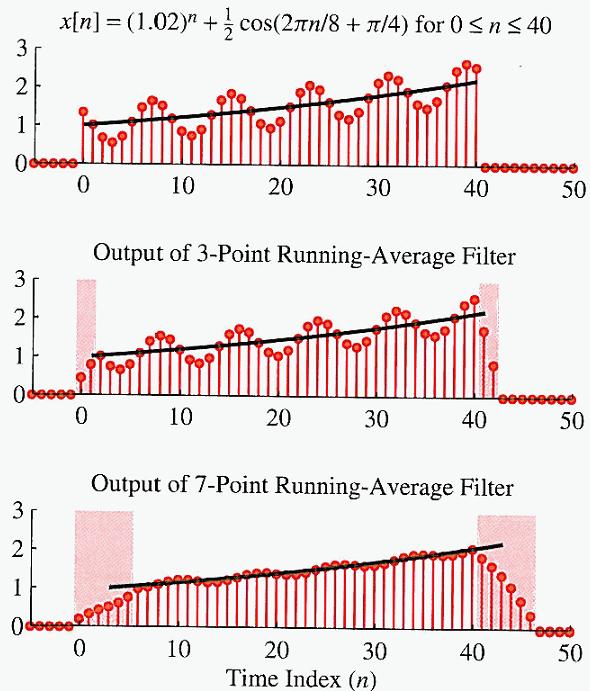
9 Example: running average filters 3-point running average filter: 7-point running average filter

10

11 Time-invariant System time-invariant system is referred to a system y[n]=t{x[n]} satisfying for all n 0. That is, when the input is delayed (shifted) by n 0, the output is delayed by the same amount.

12 Linear Time-invariant (LTI) System It can be easily verified that the FIR filter of the form is a time-invariant system. A system that is both linear and time-invariant is referred to as an LTI system. So, FIR filter is an LTI system.

13 IIR System or IIR Filter IIR filter: Linear system using both current and finite previous inputs as well as previous outputs. General form: Recursion: In IIR filter, previous outputs have been used recursively.

14 General form of LTI system It can be easily verified that IIR filter is also an LTI system. We have the definition of LTI system, but what is the general form of an LTI system? To answer this question, let us investigate what happens when we input the simplest signal, the delta function, into an LTI system. Recall: delta function (unit impulse) in discrete-time domain:

15 Impulse Response When taking the unit impulse δ[n] as input to an LTI system, the output h[n] is called the impulse response of this LTI system. Recall: Any discrete-time signal x[n] can be represented as the linear combination of delayed unit-impulse functions: x [ n] = x[ k] δ [ n k] k =

16 Impulse Response Then, we have the following property for the impulse response of an LTI system: So y = [ ] [ ] [ ] n k= = T x [ ] { [ ]} k k= T yn [ ] = xk hn k k= x δ n k δ n k k [ ] [ ] by Linearity by Timeinvariance

17 Impulse Response yn [ ] = xk hn k k= [ ] [ ] The operation is convolution. Hence, when we know the impulse response h[n] of a linear system, then the output signal can be completely determined by the input signal and the impulse response via the convolution. Knowing an LTI system equivalent to Knowing its impulse response

18 Property Response of LTI System yn [ ] = xn [ ] hn [ ] = x k h nk k= [ ] [ ] Output of an LTI system is the convolution of the input sequence and the impulse response of the LTI system. Convolution is commutative and associative:

19 Equivalent Systems Hence, we have the following equivalent systems:

20 Equivalent Systems x[n] h 1 [n] h 2 [n] h 3 [n] y[n] x[n] h 1 [n] h 2 [n] h 3 [n] y[n]

21 Convolution and Equivalent System Property Convolution is also distributive over addition: x[n] (h 1 [n] + h 2 [n]) = x[n] h 1 [n] + x[n] h 2 [n].

22 Impulse Responses of Some LTI Systems Ideal delay: h[n] = δ[n-n d ] Moving average Accumulator h [ n] h [ n] 1 = M1 + M n 0 = 0 otherwise Forward difference: h[n] = δ[n+1]δ[n] Backward difference: h[n] = δ[n]δ[n1] M 1 n M otherwise 2

23 An LTI system can be realized in different ways by separating it into different subsystems. The following systems are equivalent: Cascading Systems [ ] [ ] [ ] ( ) [ ] [ ] [ ] [ ] ( ) [ ] [ ] = + = + = n n n n n n n n n h δ δ δ δ δ δ δ δ

24 Equivalent Cascading Systems Another example of cascading systems inverse system. h [ n] = u[ n] ( δ [ n] δ [ n 1] ) = u[ n] u[ n 1] = δ [ n]

25 Causality A system is causal if it does not dependent on future inputs. That is, if x 1 [n]=x 2 [n] when n<n 0, then the output y 1 [n]=y 2 [n] when n<n 0 for all n 0. or equivalently, the output y[n 0 ] depends only the input sequence values for n n 0. What is the property of the impulse response of a causal system? Property: An LTI system is causal if and only if h[n] = 0 for all n < 0.

26 General Form of LTI Systems General LTI System Causal LTI System FIR Filter (namely, Finite Impulse Response) yn [ ] = hk xn k k= k= 0 [ ] [ ] yn [ ] = hk xn k M k= 0 [ ] [ ] yn [ ] = hk xn k [ ] [ ] IIR Filter (namely, Infinite Impulse Response) M = + [ ] [ ] [ ] [ ] y[ n] a k x n k b k y n k k= 0 k= 1 N

27 Difference Equation From the above, we can find that both FIR and IIR filters are causal LTI Systems. They are both difference equations. Difference equation: (variables are functions. y: unknown function; x: given) N k = 0 a k y [ n k] = b [ ] mx n m m= 0 Both FIR and IIR filters are solutions of difference equations. IIR filter is the case when a 0 =1. Difference equation is merely a more general form. M

28 Illustration: (infinite-long) Matrix Vector A General LTI system is of the form: yn [ ] = hk xn k k= [ ] [ ] Can be explained as a infinite-dimensional matrix/vector product y[ 3] h[0] h[ 1] h[ 2] h[ 3] h[ 4] h[ 5] x[ 3] y[ 2] h[1] h[0] h[ 1] h[ 2] h[ 3] h[ 4] x[ 2] y[ 1] h[2] h[1] h[0] h[ 1] h[ 2] h[ 3] = x[ 1] y[0] h[3] h[2] h[1] h[0] h[ 1] h[ 2] x[0] y[1] h[4] h[3] h[2] h[1] h[0] h[ 1] x[1] y[2] h[5] h[4] h[3] h[2] h[1] h[0] x[2]

29 What Happens in Frequency Domain? What is the influence in Frequency domain when input a discrete-time signal x[n] to an LTI system of impulse response h[n]? To investigate the influence, consider that an LTI system can be characterized by an infinitedimensional matrix as illustrated above. Conceptually, this matrix should have infinitelong eigenvectors. Eigen function: A discrete-time signal is called eigenfunction if it satisfies the following property: When applying it as input to a system, the output is the same function multiplied by a (complex) constant, i.e., eigenvalue.

30 Eigenfunction of LTI System Property: x[n] = e jwn is the eigenfunction of all LTI systems (w R) Pf: Let h[n] be the impulse response of an LTI system, when e jwn is applied as the input, y [ ] [ ] jw( nk ) jwn n = h k e = e h[ k] k = k = e jwk Let H ( ) jw e = h[ k] k = e jwk we can see [ ] ( ) n H e jw e jwn y =

31 Frequency Response Hence, e jwn is the eigenfunction of the LTI system; The associated eigenvalue is H(e jw ). We call H(e jw ) the LTI system s frequency response The frequency response is a complex function consisting of the real and imaginary parts, H(e jw ) = H R (e jw ) + jh I (e jw ) Physical meaning: When input is a signal with frequency w (i.e., e jwn )), the output is a signal of the same frequency w, but the magnitude and phase could be changed (characterized by the complex amplitude H(e jw ))

32 Frequency Response Another explanation of frequency response Recall the discrete-time Fourier transform (DTFT) pair: Forward DTFT Inverse DTFT

33 Frequency Response By definition, the frequency response: H ( ) jw e = h[ k] k = is just the DTFT of the impulse response h[n]. e jwk Impulse Response DTFT Inverse DTFT Frequency Response This is an important reason why we need DTFT for discrete-time signal analysis, besides the use of continuous Fourier transform.

34 LTI System and Frequency Response Now, let s go back to the problem: When input a signal x[n] to an LTI system, what happens in the frequency domain? Remember that the output of an LTI system is y[n]=x[n]*h[n], the convolution of x[n] and h[n]. In DTFT, we still have the convolution theorem: time domain convolution is equivalent to frequency domain multiplication. Hence, the output in the frequency domain is the multiplication, Y(e jw ) = X(e jw )H(e jw )

35 Multiplication in Frequency Domain In sum, the output sequence s spectrum is the multiplication of the input spectrum and the frequency response. Knowing an LTI system equivalent to equivalent to Knowing its frequency response Knowing its impulse response equivalent to

36 Application Example of Eigenfunctions Sinusoidal responses of LTI systems: A jφ jw A 0n jφ x n = Acos w0n + φ = e e + e e 2 2 [ ] ( ) jw n x [ n] x [ n] 0 + The response of x 1 [n] and x 2 [n] are [ ] ( jw = )( ) y1 n H e A/2 e 0 0 [ ] ( jw = )( ) y2 n H e A/2 e j( w n+ϕ ) j( w n+ϕ ) 0 0 The total response is y[n] = y 1 [n] + y 2 [n] 1 2

37 Example: Frequency Response of the Moving-average System Impulse response of the moving-average system is h [ n] = M M Therefore, the frequency response is 2 M 1 n otherwise M 2 H e [ ] 2 jw 1 = M 1 + M M n=m e 1 jwn

38 The following is the geometric series formula: So Geometric Series Formula 0 1, 1 m m n k n k k n k n m m n α α α α α α = = + = = > 1 0 1, 1 L L k k α α α + = =

39 Frequency Response of the Movingaverage System jw 1 H e = M + M + 1 = = = jwm1 1 e e M + M + 1 1e 2 1 ( 1) 2 ( + + ) ( + + ) 1 e e M + M + 1 1e jw M M 1 /2 jw M M 1 / ( + + ) ( + + ) 1 e e M + M + 1 e e M n=m jw M + jw e jwn jw jw M M 1 /2 jw M M 1 / jw/2 jw/2 e e ( M ) jw M + 1 /2 2 1 ( M ) jw M 2 1 /2

40 Further evaluation Frequency Response of the Movingaverage System 1 2 ( jw ) 1 2 jw ( ) ( + + ) ( + + ) jw 1 e e H e = M + M + 1 e e = = exp j H e jw M M 1 /2 jw M M 1 / ( + M + ) [ ] jw/2 jw/2 1 sin w M 1 / 2 e M + M + 1 sin w/ 2 H e ( M ) 1 2 jw M /2 2 1 e ( M ) jw M 2 1 /2 (magnitude and phase)

41 Spectrum of the Moving-average System (M 1 = 0 and M 2 = 4) Recall that, in DTFT, the frequency response is repeated with period 2π. High frequency is close to ±π. Amplitude response Phase response

42 Example: Discrete-time Ideal Low-pass Filter Ideal low-pass filter in DTFT domain H lowpass jw ( e ) 1, w < wc = 0, wc < w < π Note that we usually depict the frequency response in the range [-π,π] only, and bearing in mind that the spectrum is repeated with the period 2π.

43 Ideal Low-pass Filter in DTFT domain

44 Discrete-time Ideal Low-pass Filter The impulse response h lowpass [n] can be found by inverse Fourier transform: 1 wc jwn hlowpass[ n] = e dw 2π wc 1 jwn w 1 c jwcn jwcn = e w = ( e e ) c 2π jn 2π jn = sin wn c π n Uniform samples of Sinc function

45 Approximation of Discrete-time Ideal Low-pass Filter In other words, the forward DTFT of the sampled sync function recovers the ideal low-pass filter: jw sin wn c Hlowpass( e ) = e π n n= However, as analyzed before, the sampled sync function cannot be realized by difference equation because it reaches infinity on both ends. To approximate the ideal low-pass filter, a method is to use the partial sum instead M jw sin wn c HM ( e ) = e π n n=m jwn jwn

46 Approximation of Discrete-time Ideal Low-pass Filter Examples of M=1, 3, 7, 19

47 Ideal Frequency-selective Filters The low frequencies are frequencies close to zero, while the high frequencies are those close to ±π. Since that the frequencies differing by an integer multiple of 2π are indistinguishable, the low frequency are those that are close to an even multiple of π, while the high frequencies are those close to an odd multiple of π. Ideal frequency-selective filters: An important class of linear-invariant systems includes those systems for which the frequency response is unity over a certain range of frequencies and is zero at the remaining frequencies.

48 Frequency Response of Ideal Lowpass Filter

49 Frequency Response of Ideal Highpass Filter

50 Frequency Response of Ideal Bandstop Filter

51 Frequency Response of Ideal Bandpass Filter