The General Dirichlet Problem on a Rectangle

Transcription

1 The General Dirichlet Problem on a Rectangle Ryan C. Trinity University Partial Differential Equations March 7, 0

2 Goal: Solve the general (inhomogeneous) Dirichlet problem u = 0, 0 < x < a, 0 < y < b, u(x,0) = f (x), u(x,b) = f (x), 0 x a, u(0,y) = g (y), u(a,y) = g (y), 0 y b. Picture: u(x,b)=f (x) u(0,y)= g (y)

3 Strategy: Reduce to four simpler problems and use superposition. u(x,b)=f (x) u(0,y)=0 u(0,y)= g (y) u(x,b)=f (x) = u(0,y)=g (y)

4 Strategy: Reduce to four simpler problems and use superposition. u(x,b)=f (x) u(0,y)=0 u(0,y)= g (y) (*) u(x,b)=f (x) = u(0,y)=g (y)

5 Strategy: Reduce to four simpler problems and use superposition. (A) u(0,y)=0 u(x,b)=f (x) u(0,y)= g (y) (*) u(x,b)=f (x) = u(0,y)=g (y)

6 Strategy: Reduce to four simpler problems and use superposition. (A) u(0,y)=0 u(x,b)=f (x) (B) u(0,y)= g (y) (*) u(x,b)=f (x) = u(0,y)=g (y)

7 Strategy: Reduce to four simpler problems and use superposition. (A) u(0,y)=0 u(x,b)=f (x) (B) u(0,y)= g (y) (*) u(x,b)=f (x) = u(0,y)=g (y) (C)

8 Strategy: Reduce to four simpler problems and use superposition. (A) u(0,y)=0 u(x,b)=f (x) (B) u(0,y)= g (y) (*) u(x,b)=f (x) = u(0,y)=g (y) (C) (D)

9 Remarks: Explicitly, if u, u, u 3 and u 4 solve the Dirichlet problems (A), (B), (C) and (D) (respectively), then the general solution to ( ) is u = u + u + u 3 + u 4. Note that the boundary conditions in each of (A) - (D) are homogeneous, with the exception of a single side of the rectangle. Problems with more general inhomogeneous boundary conditions (e.g. Neumann or Robin conditions) can be reduced in a similar manner.

10 Solution to (A) and (B) We have already seen that the solution to (B) is given by u (x,y) = B n sin nπx sinh nπy a a, n= where a B n = a sinh nπb f (x)sin nπx a 0 a dx. We can likewise use separation of variables to show that the solution to (A) is where u (x,y) = A n = n= a sinh nπb a A n sin nπx a a 0 sinh nπ(b y), a f (x)sin nπx a dx.

11 Solution to (C) and (D) In the same manner we obtain the solution to (C): u 3 (x,y) = C n sinh n= nπ(a x) b sin nπy b, with b C n = b sinh nπa g (y)sin nπy b 0 b dy, as well as the solution to (D): where u 4 (x,y) = D n = n= D n sinh nπx b sin nπy b, b b sinh nπa g (y)sin nπy b 0 b dy.

12 Remarks: In each case, the coefficients of the solution are just multiples of the Fourier sine coefficients of the function giving the nonzero boundary condition, e.g. D n = sinh nπa (nth sine coefficient of g on [0,b]) b The coefficients for each boundary condition are independent of the others. If any of the boundary conditions is zero, we may omit that term from the solution. E.g. if g 0, then we don t need to include u 3.

13 Example Solve the Dirichlet problem on [0,] [0,] with the following boundary conditions. u=0 u=(-y) / u= We have a =, b = and f (x) =, f (x) = 0, g (y) = ( y), g (y) = y.

14 It follows that B n = 0 for all n, and the remaining coefficients we need are A n = sinh nπ 0 sin nπx dx = 4( + ( )n+ ) nπ sinhnπ, ( y) C n = sinh nπ sin nπy 0 dy = 4(π n + ( ) n ) n 3 π 3 sinh nπ, D n = sinh nπ 0 ( y)sin nπy dy = 4 nπ sinh nπ.

15 The complete solution is thus u = n= + + 4( + ( ) n+ ) nπ sinhnπ n= n= 4(n π + ( ) n ) n 3 π 3 sinh nπ 4 nπ sinh nπ sinnπx sinhnπ( y) sinh nπx sinh sin nπy. nπ( x) sin nπy

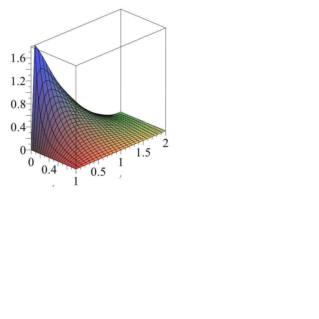
16 Graphically: =