The two-dimensional heat equation

Transcription

1 The two-dimensional heat equation Ryan C. Trinity University Partial Differential Equations March 5, 015

2 Physical motivation Goal: Model heat flow in a two-dimensional object (thin plate. Set up: Represent the plate by a region in the xy-plane and let { u(x,y,t = temperature of plate at position (x,y and time t. For a fixed t, the height of the surface z = u(x,y,t gives the temperature of the plate at time t and position (x,y. Under ideal assumptions (e.g. uniform density, uniform specific heat, perfect insulation along faces, no internal heat sources etc. one can show that u satisfies the two dimensional heat equation u t = c u = c (u xx +u yy

3 Rectangular plates and boundary conditions For now we assume: The plate is rectangular, represented by R = [0,a] [0,b]. y b a x The plate is imparted with some initial temperature: u(x,y,0 = f(x,y, (x,y R. The edges of the plate are held at zero degrees: u(0,y,t = u(a,y,t = 0, 0 y b, t > 0, u(x,0,t = u(x,b,t = 0, 0 x a, t > 0.

4 Separation of variables Assuming that u(x,y,t = X(xY(yT(t, and proceeding as we did with the -D wave equation, we find that X BX = 0, X(0 = X(a = 0, Y CY = 0, Y(0 = Y(b = 0, T c (B +CT = 0. We have already solved the first two of these problems: X = X m (x = sin(µ m x, µ m = mπ a, B = µ m Y = Y n (y = sin(ν n y, ν n = nπ b, C = ν n, for m,n N. It then follows that T = T mn (t = A mn e λ mnt, λ mn = c µ m +νn = cπ m a + n b.

5 Superposition Assembling these results, we find that for any pair m,n 1 we have the normal mode u mn (x,y,t = X m (xy n (yt mn (t = A mn sin(µ m x sin(ν n ye λ mn t. The principle of superposition gives the general solution u(x,y,t = A mn sin(µ m x sin(ν n ye λmnt. m=1 n=1 The initial condition requires that f(x,y = u(x,y,0 = n=1 m=1 ( mπ ( nπ A mn sin a x sin b y, which is just the double Fourier series for f(x,y.

6 Conclusion Theorem If f(x,y is a sufficiently nice function on [0,a] [0,b], then the solution to the heat equation with homogeneous Dirichlet boundary conditions and initial condition f(x,y is u(x,y,t = m=1 n=1 A mn sin(µ m x sin(ν n ye λ mn t, where µ m = mπ a, ν n = nπ b, λ mn = c µ m +νn, and A mn = 4 ab a b 0 0 f(x,ysin(µ m xsin(ν n ydy dx.

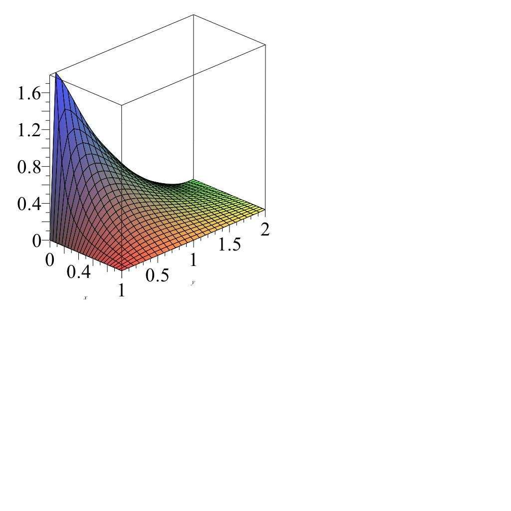
7 Example A square plate with c = 1/3 is heated in such a way that the temperature in the lower half is 50, while the temperature in the upper half is 0. After that, it is insulated laterally, and the temperature at its edges is held at 0. Find an expression that gives the temperature in the plate for t > 0. We must solve the heat problem above with a = b = and { 50 if y 1, f(x,y = 0 if y > 1. The coefficients in the solution are A mn = 4 ( mπ ( nπ f(x,ysin 0 0 x sin y dy dx ( mπ 1 ( nπ = 50 sin x dx sin y dy 0 0

8 ( (1+( 1 m+1 ( (1 cos nπ = 50 πm πn = 00 (1+( 1 m+1 (1 cos nπ π. mn Since λ mn = π m n 4 = π m 6 +n, the solution is u(x,y,t = 00 ( (1+( 1 m+1 (1 cos nπ π mn sin m=1 n=1 ( nπ y e π (m +n t/36. ( mπ sin x

9 Inhomogeneous boundary conditions Steady state solutions and Laplace s equation -D heat problems with inhomogeneous Dirichlet boundary conditions can be solved by the homogenizing procedure used in the 1-D case: 1. Find and subtract the steady state (u t 0;. Solve the resulting homogeneous problem; 3. Add the steady state to the result of Step. We will focus only on finding the steady state part of the solution. Setting u t = 0 in the -D heat equation gives u = u xx +u yy = 0 (Laplace s equation, solutions of which are called harmonic functions.

10 Dirichlet problems Definition: The Dirichlet problem on a region R R is the boundary value problem u = 0 inside R, u(x,y = f(x,y on R. Δu=0 u( x,y =f( x,y When the region is a rectangle R = [0,a] [0,b], the boundary conditions will given on each edge separately as: u(x,0 = f 1 (x, u(x,b = f (x, 0 < x < a, u(0,y = g 1 (y, u(a,y = g (y, 0 < y < b.

11 1 Solving the Dirichlet problem on a rectangle Homogenization and superposition Strategy: Reduce to four simpler problems and use superposition. u(0,y= g (y ( * u(x,b=f (x Δu= 0 u(x,0=f (x 1 u(a,y=g (y = u(0,y= 0 u(0,y=g (y 1 u(x,b=0 (A Δu= 0 u(x,0=f (x 1 u(x,b=0 (C Δu= 0 u(a,y=0 u(a,y=0 u(0,y=0 u(0,y= 0 u(x,b=f (x (B (D Δu= 0 u(x,0=0 u(x,b=0 Δu= 0 u(a,y=0 u(a,y=g (y u(x,0=0 u(x,0=0

12 Remarks: If u A, u B, u C and u D solve the Dirichlet problems (A, (B, (C and (D, then the general solution to ( is u = u A +u B +u C +u D. Note that the boundary conditions in (A - (D are all homogeneous, with the exception of a single edge. Problems with inhomogeneous Neumann or Robin boundary conditions (or combinations thereof can be reduced in a similar manner.

13 Solution of the Dirichlet problem on a rectangle Case B Goal: Solve the boundary value problem (B: u = 0, 0 < x < a, 0 < y < b, u(x,0 = 0, u(x,b = f (x, 0 < x < a, u(0,y = u(a,y = 0, 0 < y < b. Setting u(x,y = X(xY(y leads to X +kx = 0, Y ky = 0, X(0 = X(a = 0, Y(0 = 0. We know the nontrivial solutions for X are given by X(x = X n (x = sin(µ n x, µ n = nπ a, k = µ n (n N.

14 Interlude The hyperbolic trigonometric functions The hyperbolic cosine and sine functions are coshy = ey +e y, sinhy = ey e y. They satisfy the following identities: cosh y sinh y = 1, d dy coshy = sinhy, d sinhy = coshy. dy One can show that the general solution to the ODE Y µ Y = 0 can (also be written as Y = Acosh(µy+B sinh(µy.

15 Using µ = µ n and Y(0 = 0, we find Y(y = Y n (y = A n cosh(µ n y+b n sinh(µ n y 0 = Y n (0 = A n cosh0+b n sinh0 = A n. This yields the separated solutions u n (x,y = X n (xy n (y = B n sin(µ n xsinh(µ n y, and superposition gives the general solution u(x,y = B n sin(µ n xsinh(µ n y. n=1 Finally, the top edge boundary condition requires that f (x = u(x,b = B n sinh(µ n bsin(µ n x. n=1

16 Conclusion Appealing to the formulae for sine series coefficients, we can now summarize our findings. Theorem If f (x is piecewise smooth, the solution to the Dirichlet problem is u = 0, 0 < x < a, 0 < y < b, u(x,0 = 0, u(x,b = f (x, 0 < x < a, u(0,y = u(a,y = 0, 0 < y < b. u(x,y = where µ n = nπ a and B n = B n sin(µ n xsinh(µ n y, n=1 asinh(µ n b a 0 f (xsin(µ n xdx.

17 Remark: If we know the sine series expansion for f (x on [0,a], then we can use the relationship B n = 1 sinh(µ n b (nth sine coefficient of f. Example Solve the Dirichlet problem on the square [0,1] [0,1], subject to the boundary conditions u(x,0 = 0, u(x,1 = f (x, 0 < x < 1, u(0,y = u(1,y = 0, 0 < y < 1. where f (x = { 75x if 0 x 3, 150(1 x if 3 < x 1.

18 We have a = b = 1. The graph of f (x is: According to exercise.4.17 (with p = 1, a = /3 and h = 50, the sine series for f is: f (x = 450 sin ( nπ 3 π n sin(nπx. n=1

19 Homog. Dirichlet BCs Inhomog. Dirichlet BCs Homogenizing Thus, 450 sin nπ 3 π n 1 Bn = sinh(nπ and! 450 sin nπ 3, = π n sinh(nπ 450 X sin nπ 3 sin(nπx sinh(nπy. u(x, y = π n sinh(nπ n= Complete solution

20 Solution of the Dirichlet problem on a rectangle Cases A and C Separation of variables shows that the solution to (A is ( nπx ( nπ(b y u A (x,y = A n sin sinh, a a n=1 where a A n = asinh ( f nπb 1 (xsin a 0 Likewise, the solution to (C is ( nπ(a x u C (x,y = C n sinh b with n=1 C n = bsinh ( nπa b b 0 g 1 (ysin ( nπx dx. a sin ( nπy, b ( nπy dy. b

21 Solution of the Dirichlet problem on a rectangle Case D And the solution to (D is u D (x,y = D n sinh n=1 ( nπx sin b ( nπy, b where D n = bsinh ( nπa b b 0 g (ysin ( nπy dy. b Remark: The coefficients in each case are just multiples of the Fourier sine coefficients of the nonzero boundary condition, e.g. D n = 1 sinh ( nπa (nth sine coefficient of g on [0,b]. b

22 Example Solve the Dirichlet problem on [0,1] [0,] with the following boundary conditions. u=0 u=(-y / u = 0 u= We have a = 1, b = and f 1 (x =, f (x = 0, g 1 (y = ( y, g (y = y.

23 It follows that B n = 0 for all n, and the remaining coefficients we need are A n = 1 sinh ( nπ sin ( nπx dx = 4(1+( 1n+1 1 nπsinh(nπ, C n = D n = sinh ( nπ1 sinh ( nπ1 0 0 ( y ( nπy sin dy = 4(π n +( 1 n n 3 π 3 sinh ( nπ, ( ysin ( nπy dy = 4 nπsinh ( nπ.

24 The complete solution is thus u(x,y =u A (x,y+u C (x,y+u D (x,y 4(1+( 1 n+1 = sin(nπx sinh(nπ( y nπ sinh(nπ n=1 4(n π +( 1 n ( nπ(1 x + n 3 π 3 sinh ( nπ sinh n=1 4 ( nπx ( nπy + nπsinh ( nπ sinh sin. n=1 sin ( nπy

25 =