THE FOURIER TRANSFORM (Fourier series for a function whose period is very, very long) Reading: Main 11.3

Transcription

1 THE FOURIER TRANSFORM (Fourier series for a function whose period is very, very long) Reading: Main 11.3

2 Any periodic function f(t) can be written as a Fourier Series a a n cos( nωt) + b n sin n ωt n=1,2... with n=1,2... ( ) a n = 2 T T f (t)cos( nωt)dt b n = 2 T 0 T 0 f (t)sin nωt ( )dt a n b n ω ω

3 Any periodic function f(t) can be written as a Fourier Series c n e inωt + c n * e inωt n=0 or c n e inωt n= with c n = c n * c n = 1 T T 0 f (t)e inωt dt c = a 0 ; c = a n ib n ; c = a n +ib n 0 2 n 2 n 2

4 Focus on c form: f (t) = c n e inωt n= T ; ω = 2π T 0 nω ω n c n = 1 T T 0 f (t)e inωt dt c n = ω 2π f (t)e iω nt dt f (t) = n= ω f (t ')e iω n t ' dt ' 2π t '= c n e iω n t

5 f (t) = n= ω 2π f (t')e iω n t' dt t '= ' e iω n t ω dω; ω n ω; n= ω= f (t) = 1 dωe iωt 1 f (t')e iωt' dt' 2π 2π ω= t '= coefficient or Fourier transform (function of ω, not time) f (ω) = 1 2π f (t)e iωt dt

6 Fourier transform: f (ω) = 1 2π f (t)e iωt dt Inverse Fourier transform: Frequency representation f (t) = 1 2π %f (ω)e +iωt dω Time representation Fourier transform (FT) will be useful for the same reason the Fourier series was: the frequency representation allows simple multiplication, not integration!

7

8 The (Fast) Fourier Transform The Fourier transform (FT) is the analog, for non-periodic functions, of the Fourier series for periodic functions can be considered as a Fourier series in the limit that the period becomes infinite The Fast Fourier Transform (FFT) is a computer algorithm to calculate a FT for a discrete (or digitized) function input is a series of 2 p (complex) numbers representing a time function; output is 2 p (complex) numbers representing the coefficients at each frequency has a few rules to be obeyed Excel (or Maple/Mathmatica) will do this for you - it s not too hard to learn.

9 t F(t) 1 t 36 2 t 50 3 t 63 4 t 68 5 t 49 6 t 47 7 t 34 8 t 20 9 t 6 10 t t t t 1024 t Time t Τ = Ν t (all data in window)

10 1 T = f 0; 2π T = ω 0 Fundamental frequency (small!) t t 1 2 t = f N; 2π 2 t = ω N 2 t is SMALLEST period of a sinusoidal function that is sensible to consider - faster oscillations have no meaning for this function Only HALF the frequency spectrum is unique information Nyquist frequency

11 Aliasing samples function y x 4

12 The FFT c(ω) ω = ω ω ?? ω Ν

13

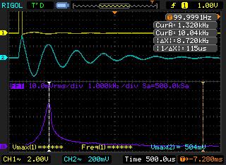
14 Damped Voltage Oscillation in LRC Circuit 0,8 0,6 0,4 Voltage (V) 0, ,005 0,01 0,015 0,02-0,2 measured voltage -0,4-0,6-0,8 Time (s) FFT Output Spectrum - Real Coeffiecients REal Coefficients T Time (s) Frequency

15 V_out (V) FFT abs(fft), V t(s) time(s) Vin Vout FFFT FFT Freq ABS value D E E E t 5.11E E E E E E fs 1.00E E E E i 3.92E sa E E E E E fs/sa 1.96E E E E i 7.84E E E E i 9.80E E E E i 1.18E E E E i 1.37E E E E i 1.57E E E E i 1.76E E E E i 1.96E E E E E E E E E i 2.35E E E E i 2.55E Freq (s-1)

16 Fourier Uncertainty Principle

17

18 Example of Fourier transform: the square sinusoidal pulse f (t) = sin ω 0 t ( )[ θ( t + 2) θ( t 2) ] f (t) t Im ω 0 f (ω) ω 0 2 2π ω

19 [ ( )]e iωt dt f (ω) = 1 2π sinω 0t θ( t + 2) θ t 2 f (ω) = 1 2π 2 2 e +iω 0t e iω 0t 2i e iωt dt Integral limits f (ω) = 1 2i 2π 2 2 Collect terms ( e +i( ω 0 ω )t e i ( ω0+ω )t)dt f (ω) = 1 2i 2π e +i ( ω 0 ω )t ( ) + e i ω0+ω i( ω 0 +ω) i ω 0 ω ( )t 2 2 Easy integral

20 i 2π f (ω) = e +i ( ω 0 ω) 2 e i ( ω 0 ω) 2 2i( ω 0 ω) limits + e i ( ω 0+ω) 2 e +i ( ω 0+ω) 2 2i( ω 0 +ω) i 2π ( ) 2 ( ω 0 ω) f (ω) = sin ω 0 ω ( ) 2 ( ) sin ω 0 +ω ω 0 +ω Back to sine form sinc form ɶf (ω) = i 2 2π sin ( ω 0 ω) 2 ( ω 0 ω) 2 ( ) 2 sin ω 0 + ω ω 0 + ω ( ) 2

21 f (ω) = i 2 2π sin( ω 0 ω) 2 ( ω 0 ω) 2 sin ( ω +ω) 0 2 ( ω 0 +ω) 2 Im ω 0 f (ω) ω 0 2 2π ω Features: Sinc function - (sinx)/x - appears, centered at ω 0. Obviously harmonic content at ω 0! Other frequencies contribute, too. Sinc function is FT of square pulse - shift is because square pulse is multiplied by sinusoidal function

22 Im ω 0 f (ω) ω 0 2 2π ω Features: Sinc function - (sinx)/x - appears, centered at ω 0. Obviously harmonic content at ω 0! Other frequencies contribute, too. Sinc function is FT of square pulse - shift is because square pulse is multiplied by sinusoidal function. Height of peak increases and width narrows as increases. Limit? Negative frequency merely gives info about phase. What about real part? What would A(ω), φ(ω) plots look like? Bandwidth theorem - a type of uncertainty principle

23 Bandwidth theorem - a type of uncertainty principle f (t) f (ω) t f (t )=θ ( t+ 2) θ ( t 2) t = t f (ω) = zero when ω 2π sin ω 2 ω 2 ω 2 = ±π ω ω t = 4π f t = 2 ω = 4π

24 Bandwidth theorem - a type of uncertainty principle f (t) f (ω) t f (t )=θ ( t+ 2) θ ( t 2) t = t f (ω) = zero when ω 2π sin ω 2 ω 2 ω 2 = ±π ω ω t = 4π f t = 2 ω = 4π