Groundwater Modeling of the NorthMet Plant Site

Transcription

1 Groundwater Modeling of the NorthMet Plant Site Supporting Document for Water Modeling Data Package Volume 2 Plant Site Prepared for Poly Met Mining Inc. January West 77th Street Minneapolis, MN Phone: Fax:

2 Groundwater Modeling of the NorthMet Plant Site January 2015 P:\Mpls\23 MN\69\ \WorkFiles\APA\Support Docs\Water Modeling Package Doc\Attachment\Plant Site\Attachment A - MODFLOW\FEISPlantSiteMODFLOWReport_v1d11.docx i Contents Acronyms and Abbreviations... v Introduction... 1 Objectives... 1 Background... 1 Report Organization... 2 Conceptual Model... 4 Geologic Units... 4 Native Unconsolidated Deposits... 4 Non-Native Deposits... 6 Bedrock... 7 Sources and Sinks for Water... 8 Local Flow System... 8 Hydrologic Model Selection... 9 Model Construction and Calibration...11 Model Grid and Layers...11 Boundary Conditions...12 Hydraulic Conductivity and Storage...13 Recharge...13 Current Conditions Model Calibration...14 Calibration Objective...15 Calibration Parameters...15 Calibration Data Sets...16 Regularization and Prior Information...18 Calibration Results...18 Assumptions and Limitations of the Model...21 Predictive Simulations...23 Modifications to the Current Conditions Model...24 Model Layers...24 Boundary Conditions...24

3 4.1.3 Hydraulic Conductivity Recharge Predictive Simulation Results Pond Seepage and Discharge to GoldSim Groundwater Flow Paths Particle Tracking Simulations Thickness of Unsaturated Zones Summary and Conclusions References...35 ii

4 List of Tables Table 2-1 Table 2-2 Table 2-3 Table 3-1 Table 3-2 Table 3-3 Table 3-4 Table 4-1 Table 4-2 Table 4-3 Table 4-4 Table 4-5 Table 4-6 Table 4-7 Hydraulic Conductivity Measured During Single-Well Pumping Tests in Unconsolidated Materials Hydraulic Conductivity Measured in 2014 in Unconsolidated Materials Using Slug Tests... 6 Hydraulic conductivity measured in bedrock during packer tests Transient Calibration Stress Periods Calibration Statistics for Observations Estimated Seepage Rates to GoldSim Groundwater Flow Paths from Current Conditions Simulation Flow Calibration Observations and Simulated Values Pond Elevations Used for Predictive Simulations Recharge Rates Used for Predictive Simulations Estimated Seepage Rates From Current Conditions and Predictive Simulations Percentage of FTB Pond Seepage Discharging to Each GoldSim Groundwater Flow Path Percentage of FTB Dam Infiltration Discharging to Each GoldSim Groundwater Flow Path Estimated Depth of Unsaturated Material in FTB Dams and Beaches Estimated Depth of Unsaturated Material below LTVSMC Tailings List of Figures Figure 3-1 Figure 3-2 Figure 4-1 Comparison of Modeled and Measured Steady-State and Transient Heads Comparison of Modeled and Measured Drawdown at Tailings Basin Piezometers Summary of Estimated Tailings Basin Flow Rates List of Large Tables Large Table 1 Large Table 2 Large Table 3 Large Table 4 Large Table 5 Large Table 6 Calibration Parameters, Parameter Bounds, and Optimized Values Steady-State Calibration Observations and Simulated Values Transient Head Calibration Observations and Simulated Values Transient Drawdown Calibration Observations and Simulated Values Hydraulic Conductivity Values Used for Flotation Tailings in Predictive Simulations Beach Seepage Directions by Percent of Flow to Each Flow Path iii

5 List of Large Figures Large Figure 1 Site Layout Large Figure 2 NorthMet Bulk Tailings 2005 Permeability Test Results Large Figure 3 Model Domain and Grid Large Figure 4 Layer 2 Thickness Large Figure 5 Model Boundary Conditions Layers 1 and 2 Large Figure 6 Hydraulic Conductivity Zones in Layer 1 Large Figure 7 Hydraulic Conductivity Zones in Layer 2 Large Figure 8 Recharge Zone Extents First Active Layer Large Figure 9 Calibration Observation Locations Large Figure 10 Simulated Groundwater Head Contours and Head Residuals in Layer 1 Large Figure 11 Simulated Groundwater Head Contours and Head Residuals in Layer 2 Large Figure 12 Observed vs Simulated Drawdown: DH96-28, DH96-30, DH96-32, DH96-37 Large Figure 13 Observed vs Simulated Drawdown: PN1J-99, F-2, P2HA-99, P2HB-99 Large Figure 14 Observed vs Simulated Drawdown: P1H1-99, P1H-99, P3H1-99, P2H1-99 Large Figure 15 Observed vs Simulated Drawdown: P3H-99, DNR-1, DNR-2, DNR-3 Large Figure 16 Observed vs Simulated Drawdown: DNR-4, DNR-5, DNR-6, GW004 Large Figure 17 Observed vs Simulated Drawdown: GW005, A-1, A-3, A-9 Large Figure 18 Observed vs Simulated Drawdown: B-2, D-1, D-4, G-2 Large Figure 19 Flotation Tailings Basin Configuration - Mine Year 1 Large Figure 20 Flotation Tailings Basin Configuration - Mine Year 7 Large Figure 21 Flotation Tailings Basin Configuration - Mine Year 8 Large Figure 22 Flotation Tailings Basin Configuration - Mine Year 18 and 20 Long-term Closure Large Figure 23 Mine Year 1 Boundary Conditions - Layer 1 Large Figure 24 Mine Year 7 Boundary Conditions - Layer 1 Large Figure 25 Mine Year 8 Boundary Conditions - Layer 1 Large Figure 26 Long-term Closure Boundary Conditions - Layer 1 Large Figure 27 Bottom Layer Boundary Conditions - Predictive Simulations Large Figure 28 Fate and Transport of Infiltration - Current Conditions Large Figure 29 Fate and Transport of Tailings Basin Infiltration - Mine Year 1 Large Figure 30 Fate and Transport of Tailings Basin Infiltration - Mine Year 7 Large Figure 31 Fate and Transport of Tailings Basin Infiltration - Mine Year 8 Large Figure 32 Fate and Transport of Tailings Basin Infiltration - Mine Year 18 Large Figure 33 Fate and Transport of Tailings Basin Infiltration - Mine Year 20 Large Figure 34 Fate and Transport of Tailings Basin Infiltration - Long-term Closure iv

6 Acronyms and Abbreviations Acronym Abbreviation, or Unit CDSM cfs DEIS FEIS FTB gpm HRF LTVSMC MDNR MPCA MSL SDEIS USGS Description cement deep soil mixing cubic feet per second Draft Environmental Impact Statement Final Environmental Impact Statement Flotation Tailings Basin gallons per minute Hydrometallurgical Residue Facility LTV Steel Mining Company Minnesota Department of Natural Resources Minnesota Pollution Control Agency mean sea level Supplemental Draft Environmental Impact Statement U.S. Geological Survey v

7 1.0 Introduction This report describes the technical approach, rationale, and scope for groundwater flow modeling that was conducted for the Poly Met Mining Inc. (PolyMet) NorthMet Project (Project) Plant Site. The groundwater modeling was completed to support the probabilistic modeling used to estimate Project water balances and water quality impacts presented in the NorthMet Project Water Modeling Data Package Volume 2 Plant Site (Reference (1)). This report describes the objectives of the groundwater modeling, the site conceptual model, the modeling methodology, and the modeling results. The modeling was based on the current understanding of the Plant Site conditions and the project description (Reference (2)) developed for the Final Environmental Impact Statement (FEIS). In this report, the Flotation Tailings Basin (FTB) is the newly constructed Flotation Tailings impoundment and the Tailings Basin is the existing LTV Steel Mining Company (LTVSMC) Tailings Basin as well as the combined LTVSMC Tailings Basin and the FTB. 1.1 Objectives The primary objectives for the Plant Site groundwater flow modeling were to: estimate the seepage loss from the LTVSMC Tailings Basin ponds under current conditions and the FTB pond(s) during operations and long-term closure estimate the average annual infiltration rate throughout the Tailings Basin under current conditions estimate the discharge rate of seepage entering each of the five groundwater flow paths represented in the GoldSim model (Reference (1), Reference (3) during current conditions, operations and long-term closure estimate what proportion of the water that infiltrates the various material types present at the surface of the Tailings Basin ultimately reports to each of the GoldSim groundwater flow paths estimate the depth of the phreatic surface within each of the material types present at the surface of the Tailings Basin A series of groundwater models were developed to meet these objectives. These models were designed to simulate current conditions, conditions during operations, and conditions during long-term closure. 1.2 Background The Tailings Basin, covering an area of approximately 2,600 acres (about 4 square miles), was previously used by LTVSMC and its predecessor Erie Mining Company for disposal of taconite tailings. The facility is unlined and was constructed in stages beginning in the 1950 s. Taconite tailings were deposited from 1957 to January of 2001, when the Tailings Basin was shut down. It has been inactive since then except for reclamation activities consistent with the Minnesota Department of Natural Resources (MDNR) approved 1

8 closure plan currently managed by Cliffs Erie, and more recently, activities associated with the April 6, 2010, Consent Decree between Cliffs Erie and the Minnesota Pollution Control Agency (MPCA).There are three discrete cells in the LTVSMC Tailings Basin, Cells 1E, 2E, and 2W, as shown on Large Figure 1. Cell 2W is the largest (1,447 acres) and has the highest elevation of the three cells, with an average fill height of 200 feet (approximately 1,725 feet mean sea level (MSL)). Cell 2W is currently the driest of the cells and has gradually lost the ponded water that remained following taconite processing. Cell 1E is approximately 980 acres and rises approximately 125 feet above the surrounding ground level (approximately 1,650 feet MSL); Cell 2E is about 620 acres and has the lowest elevation of all of the existing cells, rising approximately 60 feet above surrounding ground level (approximately 1,555 feet). Cells 1E and 2E currently contain ponded water. The existing Tailings Basin does not have an overflow or discharge structure. Ore processing associated with the Project will produce two types of mineral waste: Hydrometallurgical Residue and Flotation Tailings. These two wastes will be disposed of in separate facilities. Hydrometallurgical Residue will be stored in the Hydrometallurgical Residue Facility (HRF), a lined basin constructed on top of the Emergency Basin located near the southwestern corner of the Tailings Basin (Reference (4)). The FTB will be constructed in stages atop existing Cells 1E and 2E of the Tailings Basin for disposal of Flotation Tailings. FTB staging and sequencing is described in Reference (5). The FTB design includes seepage capture systems (the FTB Containment System and the FTB South Seepage Management System), as described in Reference (6). During the Draft Environmental Impact Statement (DEIS) process, a series of numerical groundwater flow models were developed for the Tailings Basin (Attachment A-6 of Reference (7), Attachment A-6 of Reference (7)). The DEIS versions of the model calibrations were steady-state and did not simulate changes in water levels within the basin. However, after LTVSMC operations and deposition of tailings ceased in 2001, the groundwater mound beneath the Tailings Basin began to dissipate, and the quantity of seepage leaving the Tailings Basin area has decreased. As part of the modeling effort for the Supplemental Draft Environmental Impact Statement (SDEIS), the calibration of the groundwater model was updated to represent transient conditions following LTVSMC closure until present, and to simulate the observed dissipation of the groundwater mound beneath the basin. For the FEIS modeling effort, the groundwater models were updated to incorporate groundwater elevation data collected through 2013 and changes as recommended by the Co-lead Agencies. This report documents the current version of the models developed for the FEIS. FTB seepage capture systems were not simulated using the models described in this report. Additional groundwater modeling was conducted to support the design of the FTB Containment System. That modeling used results from the groundwater flow modeling described in this report and is described under separate cover in Attachment C of Reference (6). 1.3 Report Organization This report is organized into five sections, including this introduction. Section 2.0 presents the conceptual model of hydrogeology at the Plant Site. Section 3.0 discusses the modeling approach and calibration 2

9 methods and results. Predictive simulations of operations and long-term closure conditions are presented in Section 4.0. A report summary and conclusions are presented in Section

10 2.0 Conceptual Model A hydrogeologic conceptual model is a schematic description of how water enters, flows through, and leaves the groundwater system. Its purpose is to describe the major sources and sinks of water, the grouping or division of hydrostratigraphic units into aquifers and aquitards, the direction of groundwater flow, the interflow of groundwater between aquifers, and the interflow of water between surface waters and groundwater. The hydrogeologic conceptual model is both scale-dependent (e.g., local conditions may not be identical to regional conditions) and dependent upon the objectives. It is important when developing a conceptual model to strive for an effective balance: the model should be kept as simple as possible while still adequately representing the system to analyze the objectives at hand. 2.1 Geologic Units This section provides an overview of the Plant Site geology and the hydraulic properties of each geologic unit, particularly as they pertain to the development of the groundwater flow models. A more detailed summary of the current understanding of bedrock structure and hydrogeology at the Mine Site and the Plant Site, and description of the regional and local bedrock geology and hydrogeology, including the nature of fractured bedrock, can be found in Reference (8) Native Unconsolidated Deposits The native unconsolidated deposits in the vicinity of Plant Site are a relatively thin mantle of Quaternaryage glacial till and associated reworked sediments, most of which were deposited and reworked by the retreating Rainy Lobe during the last glacial period in association with the development of the Vermillion moraine complex (Reference (9))). Near the Tailings Basin, unconsolidated deposits have been characterized based on soil borings and monitoring wells, which have been completed to the north and west of the Tailings Basin. The unconsolidated deposits generally consist of discontinuous lenses of silty sand to poorly graded sand with silt, to poorly graded sand with gravel. Very little silt or clay has been encountered, with the exception of the soil boring drilled near monitoring well GW006, where several feet of silt is interbedded with silty sand (Reference (10)). In places, the till is overlain by organic peat deposits. Depth to bedrock in the area surrounding the Tailings Basin is generally less than 50 feet. The unconsolidated deposits generally thicken in a northerly direction toward the Embarrass River. Wetland areas also become more common to the north, off the northern flank of the Giant s Range, the granite outcrops located adjacent to the Tailings Basin. These wetland areas are underlain by thin glacial drift and lacustrine deposits, which were deposited by the retreating Rainy Lobe and associated lakes that were trapped between the retreating ice margin and the Giant s Range. Siegel and Ericson (Reference (11)) indicate that the till of the Rainy Lobe has an estimated hydraulic conductivity range of 0.1 to 30 feet/day. In-situ pumping tests were conducted at monitoring wells GW001, GW006, GW007, GW009, GW010, GW011, and GW012 to estimate hydraulic conductivity, as described in detail in Attachment F of Reference (12). The data collected during the tests was used to estimate the hydraulic conductivity of the unconsolidated deposits using three different methods; the Moench solution (Reference (13)), the Theis solution (Reference (14)), and using specific capacity data (Reference (15)). The hydraulic conductivity estimates from each solution are different at each location. 4

11 Not only is there spatial variability, shown by differences between wells, but there is uncertainty in the hydraulic conductivity at any given well, shown by the differences in the estimates at each well. Table 2-1 shows the estimates of hydraulic conductivity at each well (Reference (10)). GW009 generally has the lowest estimates of hydraulic conductivity (around 0.5 feet/day) and GW010 generally has the highest estimates of hydraulic conductivity (around 50 feet/day). The arithmetic and geometric means of the average hydraulic conductivity at the test locations are approximately 13 feet/day and 5 feet/day, respectively. Table 2-1 Hydraulic Conductivity Measured During Single-Well Pumping Tests in Unconsolidated Materials. Monitoring Well (1) Reference (13) (2) Reference (14) Moench Solution (1) (feet/day) Theis Solution (2) (feet/day) Specific Capacity (feet/day) GW GW GW GW GW GW GW Additional characterization of hydraulic properties of the unconsolidated deposits was conducted as part of a geotechnical investigation during 2014 (Attachment F of Reference (12)). Slug tests were conducted in ten standpipe piezometers and two monitoring wells screened in the native unconsolidated deposits: R14-04, R14-06, R14-08, R14-12, R14-13, R14-15, R14-16, R14-26, R14-27, R14-28, GW001, and GW012. Hydraulic conductivity estimates from the slug tests ranged from 0.15 to 132 feet/day. The results of those analyses are shown in Table

12 Table 2-2 Well R14-04 R14-06 R14-08 R14-12 R14-13 R14-15 R14-16 R14-26 R14-27 R14-28 GW001 GW012 Hydraulic Conductivity Measured in 2014 in Unconsolidated Materials Using Slug Tests Test K feet/day test 3 - in 2.86 test 3 - out 3.57 test 2 - out test 3 - out test 1 - in 1.19 test 2 - out 1.42 test 1 - out 0.15 test 2 - out 0.16 test 2 - out 2.12 test 3 - in 1.53 test 1 - in test 2 - out test 2 - out test 3 - in test 2 - out test 3 - in test 2 - out test 3 - out test 1 - in 0.38 test 2 - out 0.77 test 1 - in 0.99 test 3 - out 1.24 test 1 - in 0.44 test 2 - in Non-Native Deposits The Tailings Basin is composed of interbedded layers of LTVSMC tailings, which are generally coarser near the dams and finer in the center of the cells. The hydraulic properties of the LTVSMC tailings vary over several orders of magnitude and are primarily a function of the grain-size distribution of the deposits. The hydraulic properties of LTVSMC tailings have been estimated using multiple methods and are described in additional detail in Reference (12). Geotechnical modeling used hydraulic conductivity estimates of feet/day for LTVSMC fine tailings and 6.9 feet/day for coarse tailings (Reference (12)). 6

13 The hydraulic conductivity of the Flotation Tailings has been estimated using falling-head permeability testing conducted at a range of confining pressures. As shown on Large Figure 2, testing results indicate that hydraulic conductivity decreases significantly with increasing confining pressure. Geotechnical modeling of the FTB uses three representative values of hydraulic conductivity for the Flotation Tailings: 0.5 feet/day for shallow tailings, 0.2 feet/day for intermediate tailings, and 0.06 feet/day for deep tailings (Reference (12)). As described in Section 4.1.3, the relationship between hydraulic conductivity and depth shown on Large Figure 2 was used to define the hydraulic conductivity of the Flotation Tailings in the MODFLOW models Bedrock The uppermost bedrock at the Plant Site consists of quartz monzonite and monzodiorite of the Neoarchean Giant s Range batholith. These pink to dark-greenish gray, hornblende-bearing, coarsegrained rocks are referred to collectively as the Giant s Range granite. The granite locally outcrops as a northeast-southwest trending ridge and drainage divide that makes up the highest topography in the area; the Giant s Range. The Giant s Range granite has been scoured by glaciers, creating local depressions and linear valleys. In this report, bedrock hills is used to describe the Giant s Range granite outcrops located adjacent to the Tailings Basin. Groundwater flow within the bedrock is primarily through fractures and other secondary porosity features, as the rock has low primary hydraulic conductivity. The upper portions of the rock are more likely than rock at depth to contain a fracture network capable of transmitting water. The literature-based assessment of the upper fractured zone suggests that groundwater flow in the Giants Range granite likely occurs mostly in the upper 300 feet of the bedrock; however, the site-specific fracture data indicate that the amount of fracturing decreases significantly in the upper 20 feet of the bedrock surface (Reference (8)). Siegel and Ericson (Reference (11)) measured specific capacity in one well in the upper 200 feet of the Giant s Range granite and measured hydraulic conductivity of 2.6 x 10-2 feet/day. This well was located less than 1 mile to the east of the Plant Site. Specific capacity data from a residential well located north of the Plant Site suggests that the hydraulic conductivity of the upper 47 feet of the granite at that location is approximately 42 feet/day. The log for this well indicates that the top of bedrock is at 18 feet below grade, and the casing also extends to 18 feet below grade. Because the well casing apparently does not extend into bedrock, it is possible that the higher hydraulic conductivity estimate at this well may reflect some degree of hydraulic connection with the unconsolidated deposits. Packer testing was conducted at five boreholes in the uppermost portions (<20 feet) of the Giant s Range granite during a 2014 geotechnical investigation in the Plant Site area (Appendix F of Reference (12)). The results from that testing are shown on Table 2-3. Hydraulic conductivity values for the upper portion of the Giant s Range granite at the Plant Site range from effectively zero (i.e., no water was produced in three of the packer test intervals) to 3 feet/day, with a geometric mean of 0.14 feet/day (for the purposes of calculating a geometric mean, the lowest hydraulic conductivity value measured during the investigation was used for the three intervals that did not produce water). 7

14 Table 2-3 Hydraulic conductivity measured in bedrock during packer tests. Boring Test Interval (feet) K r feet/day B14-36 B < (1) < (1) B14-44 B < (1) B (1) For packer test results where zero inflow was observed during testing, permeability values were selected based on inference from lowest packer test result obtained. 2.2 Sources and Sinks for Water The Tailings Basin receives water from direct precipitation and runoff from watershed areas to the east. Water falling within the Tailings Basin watershed collects in the ponds in Cell 1E and Cell 2E or infiltrates through dams and beaches. The ponds lose water to evaporation from the water surface and to seepage through the pond bottom. Most groundwater in the Plant Site vicinity flows to the north and northwest toward the Embarrass River; however, some portion of the water entering the Tailings Basin flows south and discharges to Second Creek, a tributary of the Partridge River. 2.3 Local Flow System Regionally, groundwater flows primarily northward, from the bedrock hills to the Embarrass River (Reference (11)). Groundwater elevations in the network of monitoring wells located around the Tailings Basin indicate that groundwater in the unconsolidated deposits flows primarily to the north and northwest, toward the Embarrass River. Groundwater flow to the south and east is constricted by bedrock outcrops of the Giant s Range granite (Reference (5)). However, a gap in the bedrock hills near the southern end of the Tailings Basin allows some water to flow southward (south seeps), forming the headwaters of Second Creek (also known locally as Knox Creek), a tributary to the lower Partridge River. A second gap in the bedrock hills is present near the eastern side of the Tailings Basin. Under current conditions, seepage does not flow from the Tailings Basin to the east, because the Cell 1E pond is topographically lower than the surface water features to the east. Groundwater in the native unconsolidated material currently flows to the northwest toward the Tailings Basin. Following the completion of the FTB East Dam, groundwater within the unconsolidated deposits is generally expected to continue to flow from the east toward the Tailings Basin. The presence of the FTB Pond will not alter the existing regional groundwater flow direction, but may result in radial flow away from the Tailings Basin 8

15 area on a local scale. Some water could seep through the unconsolidated material below the East Dam. Based on topography and the inferred groundwater divides to the area east of the Tailings Basin, this seepage would likely discharge near the toe of the East Dam, and it is not anticipated to flow east toward the Area 5NW pit or Spring Mine Lake (Reference (16)). As part of the Project, a seepage containment system will be constructed in this area to capture any seepage that would discharge in this area (Reference (6)). As the Tailings Basin was built up over time, a groundwater mound formed beneath the basin due to seepage from the basin ponds, altering local flow directions and rates. Therefore, the Tailings Basin determines patterns of runoff and infiltration at the Plant Site. Under current conditions, water that infiltrates through the Tailings Basin (from precipitation and seepage from the existing ponds) seeps downward to the native unconsolidated deposits. Beneath the unconsolidated deposits, low-permeability crystalline bedrock impedes further downward groundwater flow; based on the contrast in hydraulic conductivity between the unconsolidated deposits and bedrock described above, groundwater flow through the bedrock is likely negligible relative to flow through the unconsolidated deposits. Because the unconsolidated deposits are thin and have relatively low hydraulic conductivity, and because the water table is close to the ground surface (which effectively limits the hydraulic gradient), the unconsolidated deposits have a limited capacity to transport Tailings Basin seepage. Therefore, a large portion of that seepage discharges to wetland areas near the Tailings Basin dams, while a small portion remains in the unconsolidated deposits and flows away from the basin laterally as groundwater. 2.4 Hydrologic Model Selection Groundwater flow was simulated with the numerical code MODFLOW-SURFACT (Reference (17)), a flow and transport code based on the U.S. Geological Survey (USGS) groundwater modeling code MODFLOW. MODFLOW was developed by the USGS and is in the public domain. Advantages of MODFLOW-SURFACT over MODFLOW that are pertinent to this modeling work include simulation of unsaturated flow, which reduces model instability due to dry model cells, and adaptive time stepping, which improves solver convergence. MODFLOW-SURFACT simulates the three-dimensional movement of water in a variably saturated system using Equation 1: Equation 1 9

16 Where: x, y, and z are Cartesian coordinates (L) K xx, K yy, and K zz are the principal components of hydraulic conductivity along the x, y, and z axes, respectively (LT -1 ) k rw is the relative permeability, which is a function of water saturation h is the hydraulic head (L) W is a volumetric flux per unit volume and represents source and/or sinks of water (T -1 ) is the drainable porosity taken to be equal to the specific yield, S y S w is the degree of saturation of water, which is a function of the pressure head S s is the specific storage of the porous material (L -1 ) t is time (T) Pseudo-soil relations were used to define the relative permeability (k rw ) and the degree of saturation (S w ). It is not necessary to explicitly include information on soil water retention to use pseudo-soil relations. The particle-tracking code MODPATH (Reference (18)) was used in the predictive simulations. MODPATH uses output files from MODFLOW simulations to compute three-dimensional flow paths by tracking particles throughout the model domain until they reach a boundary, enter an internal source or sink, or are terminated in a process specified by the modeler. MODPATH also tracks the time-of-travel for simulated particles as they move though the model domain. The graphical user interface Groundwater Vistas (Versions 6) (Reference (19)) was used to support the development of the MODFLOW models, although some elements of the models were developed outside of Groundwater Vistas. 10

17 3.0 Model Construction and Calibration The conceptual model of the Tailings Basin hydrogeology outlined in Section 2.0 was used to develop a series of numerical simulations for this study. A simulation of conditions since LTVSMC operations ceased in 2001 through December 2013 was used to calibrate model parameters. This simulation is referred to as the current conditions model in the discussion that follows. Separate predictive simulations (i.e., forward simulations) were developed for various stages of operations and for long-term closure conditions. 3.1 Model Grid and Layers The active area of the finite-difference grid covers approximately 18 square miles (Large Figure 3), extending from the Embarrass River in the north and west, to the south and east of the former LTVSMC mine pits. The model area is sufficiently large that the model boundaries do not meaningfully affect the model results at the Tailings Basin (Attachment A-6 of Reference (20)). The model grid was refined in the area of interest, with the final grid coarser at the boundaries and outside of the area of interest (cells of approximately 820 feet on a side) and more refined at the Tailings Basin (cells of approximately 100 to 200 feet on a side). The current conditions models have two layers. Layer 1 is modeled as unconfined and represents the LTVSMC tailings. Layer 2 is modeled as confined and represents the native unconsolidated deposits (glacial drift and peat) and the bedrock hills adjacent to the Tailings Basin. The portions of Layer 1 outside of the footprint of the Tailings Basin were inactivated (i.e., converted to no-flow cells). The bedrock was assumed to have a significantly lower value of hydraulic conductivity than the native unconsolidated deposits and, as such, was treated as a no-flow boundary. The exception to this was in the area of the bedrock hills, where the water table is likely located within the bedrock. In this area, the bottom of Layer 2 was lowered, and the bedrock was simulated as a zone of low hydraulic conductivity. This was necessary to prevent dry cells in Layer 2. The top elevation for Layer 1 is flat and set at an elevation of feet MSL (or 600 meters, an even increment in metric units, the standard units used to develop the models), which is above the highest elevation in the active model domain. Because Layer 1 is defined as unconfined, the water levels calculated by the model (rather than the top of Layer 1) are used to calculate transmissivity, so the elevation of the top of Layer 1 has no bearing on the simulation results. The bottom elevation for Layer 1 (equal to the top of Layer 2) was defined as the pre-mining topography, using topographic information from the USGS (Reference (21), Reference (22), Reference (23), Reference (24)). The bottom elevation for Layer 2 was defined as the top of bedrock. Bedrock elevations were calculated using a combined bedrock data set, derived from a regional, 30-meter resolution MGS bedrock surface (Reference (25)), into which local bedrock data were incorporated. Groundwater wells and borings completed in the vicinity of the Tailings Basin, at which estimated bedrock elevations were available, were buffered a distance of 3,280.8 feet (or, 1,000 meters, an even increment in metric units, the standard units used to develop the models). The area within the buffer was then clipped from the MGS bedrock surface. Finally, the coordinates of each well, its associated bedrock elevation, and the remaining regional grid data were provided as input to a new surface interpolation. The resulting surface matches the regional grid outside 11

18 the 3,280.8-feet buffer and within, smoothly transitions to match the field-measured site data. In areas where top of bedrock elevations were above 1,587 feet MSL, (which occurred in bedrock outcrop areas), the bottom of Layer 2 was assigned an elevation of 1,587 feet MSL. In addition, the bottom of Layer 2 was lowered in some areas of the model so that cells in Layer 2 had a minimum thickness of 16.4 feet. The thickness of Layer 2 is presented in Large Figure Boundary Conditions Boundary conditions were used to represent surface-water features within the model domain (Large Figure 5). Streams and rivers were simulated as specified-head boundaries in Layer 2 with elevations obtained from USGS 7.5 quadrangle maps (Reference (21), Reference (22), Reference (23), Reference (24)). The ponds in Cells 1E and 2E were simulated as specified-head boundaries in Layer 1, using water levels reported in the East Range Hydrology Study (Reference (26)) for the current conditions simulation and FTB design elevations for the future conditions simulations. The Cell 1E pond elevation was set at 1,653 feet MSL and Cell 2E pond elevation was set at 1,560 feet MSL for part of the current conditions simulation and allowed to vary between stress periods as calibration parameters for the remainder of the simulation (see Section 3.5 for calibration details). The allowed range of elevations was within the observed elevation range for each pond (Reference (26)). The River Package in MODFLOW was used to simulate the wetlands surrounding the Tailings Basin as head-dependent flux boundaries. River cells allow water to flow into and out of the boundary, with the flux dependent on a user-specified conductance and the head gradient between the boundary (a constant, user-specified stage) and the aquifer. The extent of wetlands areas was set based on delineated wetlands, including the results of site surveys, where available (Reference (27)), and National Wetland Inventory data (NWI) for the remainder of the model domain. A model cell was assigned as a river cell if at least 20% of the cell area was covered by wetlands greater than 5 acres in area. River cell stages were set at the average ground surface elevation within the model cell, calculated from regional LiDAR data (Reference (28)). The bottom elevation for each river cell was set at 3.3 feet below the assigned stage. Conductance was treated as an adjustable parameter during model calibration. In MODFLOW, the conductance of a river cell is defined by Equation 2 (Reference (29)): KA C RIV M Equation 2 Where: K = Vertical hydraulic conductivity of wetland sediment [L/T] A = Area covered by wetlands within model cell [L 2 ] M = Thickness of wetland bottom sediment [L] An initial conductance value was assigned as the cell area by assuming the thickness (M) term of the equation was equal to 3.28 feet (thickness of 1 meter in the standard model units), and the hydraulic conductivity term (K) was assigned a value of 3.28 feet/day (1 meter/day in the standard model units). During calibration, the vertical hydraulic conductivity of the wetland sediment (K) was varied, and the 12

19 initial conductance value was multiplied by the updated value of the vertical hydraulic conductivity to calculate the conductance for each river cell. Two wetland zones were defined in the model: one for cells where wetlands overlay native unconsolidated deposits, and one for cells where wetlands overlay bedrock. The vertical hydraulic conductivity values of the wetland sediments for the two zones were allowed to vary independently during model calibration to allow for different hydraulic characteristics. The south seeps were simulated using the Drain Package in MODFLOW, with the elevation of the drain cells set equal to the current elevation of the seeps, and the conductance value adjusted during calibration. Additional drain cells, representing potential seeps from bedrock outcrops, were added along the northern side of the bedrock hills. Each drain cell was assigned a head value equal to the average ground surface within that cell as calculated from regional LiDAR data (Reference (28)). Conductance values of the drain cells were adjusted during model calibration. Assuming the hydraulic conductivity values of all drain cells representing potential bedrock seeps were equal, the conductance values were proportional to the drain cell area. During model calibration, the conductance for cells with an area of 51,260 ft 2 (i.e., the majority of the drain cells representing potential bedrock seeps) was adjusted, and the conductance for the remaining drain cells representing bedrock seeps were tied to the calibrated value (i.e., conductance was scaled based on cell area). 3.3 Hydraulic Conductivity and Storage A total of eight zones were used in the current conditions model to simulate the varying geologic materials and LTVSMC tailings. The spatial distribution of hydraulic conductivity and storage zones coincided. A separate zone was used to represent the fine and coarse LTVSMC tailings in each of the three tailings basin cells (Large Figure 6), for a total of six zones in Layer 1. The fine tailings zones were generally within the centers of the cells, and the coarse tailings zones were generally around the cell perimeters in beach and dam areas. In Layer 2, one zone was used to represent the native unconsolidated deposits, and one zone was used to represent the bedrock hills (Large Figure 7). The location of the hydraulic conductivity zone defining the bedrock hills is consistent with Attachment A-6 of Reference (20) and includes gaps in the bedrock to the east and south of the Tailings Basin. Horizontal and vertical hydraulic conductivity and storage values for all eight zones were adjusted during model calibration. The LTVSMC tailings, native unconsolidated deposits, and bedrock were simulated as anisotropic. Specific yield and storativity were assigned for the LTVSMC tailings zones in Layer 1 because Layer 1 was simulated as unconfined. Because Layer 2 is defined as confined, storativity was the only storage parameter assigned to the native unconsolidated deposits and bedrock in Layer Recharge The MODFLOW Recharge Package was used to simulate the infiltration of precipitation within the model domain. Recharge was applied to the uppermost active layer. Five zones were used in the steady-state model to simulate spatially variable recharge (Large Figure 8). Two zones were used to represent recharge to the fine and coarse LTVSMC tailings in Cell 2W. One zone was used to represent the coarse LTVSMC 13

20 tailings in Cell 1E, Cell 2E, and the native unconsolidated deposits. The pond footprints in Cells 1E and 2E were represented with a zone receiving 0 inches/year of recharge, because pond seepage occurs via flux to and from the specified head cells used to simulate the ponds. The bedrock hills were represented with a single recharge zone, which matched the spatial extent used for hydraulic conductivity and storage. In the steady-state portion of the current conditions model, the two zones used to represent Cell 2W (coarse and fine tailings) were assigned higher recharge rates than during the transient portion of the simulation to reproduce the groundwater mound beneath the basin that formed during LTVSMC operations as new tailings were deposited. In the transient current conditions model, these zones were replaced with separate zones of identical extent, but lower recharge rates. The recharge applied to Cell 2W during the transient portion of the current conditions simulation was representative of conditions in Cell 2W following the end of LTVSMC operations. The recharge rates applied to Cell 2W during the steady-state portion of the simulation may not be representative of actual recharge rates during that time period; rather, they were calibrated to obtain the initial conditions for the transient portion of the simulation. The other three recharge zones and values were the same in the steady-state and transient models. Recharge rates for all zones, except the one representing the Cell 1E and Cell 2E ponds, were allowed to vary during the model calibration process. 3.5 Current Conditions Model Calibration The current conditions model simulates: (1) conditions shortly after LTVSMC operations ceased, when a larger groundwater mound was present beneath the Tailings Basin and (2) the subsequent transient dissipation of the groundwater mound over a period of approximately twelve years. The initial stress period in the simulation was steady-state, though the steady-state stress period is simulating a system that was not actually at a steady state. The steady-state simulation was used to establish the initial conditions for the transient portion of the simulation. The steady-state portion of the calibration uses groundwater elevation data from February 2002, which are representative of the period shortly after LTVSMC operations at the Tailings Basin ceased and coincides with the time period that was evaluated as part of the East Range Hydrology Project (Reference (26)). The heads from the steady-state portion of the current conditions simulation were then used as the initial heads for the transient portion of the simulation. The transient portion of the simulation spans 3,729 days (11.9 years) between February 1, 2002 and December 31, 2013 and is subdivided into seven stress periods (Table 3-1). The stress periods were defined based on measured pond elevations from the East Range Hydrology Study (Reference (26)), which includes data through 2003, and were chosen to coincide with periods of time with minimal pond level fluctuation. The period from 2003 to the end of 2013 was simulated using a single stress period. 14

21 Table 3-1 Transient Calibration Stress Periods Stress Period Length (days) Interval (years) Model calibration was completed using the automated calibration software PEST (Reference (30), Reference (31)), providing the starting point for the predictive simulations discussed in Section 4.0. Through systematic adjustment of model parameters within a user-specified range, PEST attempts to minimize the difference between observed and modeled values Calibration Objective The objective of the model calibration was to minimize the difference between observed and simulated values (i.e., residuals) for a variety of different types of calibration observations. When using PEST, the difference between observed and simulated values is quantified as the sum of squared weighted residuals and is termed the objective function or phi. Therefore, the goal of the calibration was to minimize the objective function. Calibration observations were grouped by type (i.e., steady-state head, transient head, drawdown, and seepage), and observations were assigned weights so that the contribution of each observation group to the initial objective function was roughly equal. In addition to minimizing the objective function, the model calibration was considered acceptable if the following criteria were met: the absolute residual mean was less than 15% of the observed range in heads the modeled seepage rates approximated estimates of seepage from the ponds in Cells 1E and 2E and the discharge from the south seeps widespread areas of simulated heads significantly above the ground surface in the model area of interest did not result Calibration Parameters The calibration included 54 adjustable parameters in the following seven parameter groups: horizontal hydraulic conductivity of tailings material, native unconsolidated deposits, and bedrock 8 parameters 15

22 vertical hydraulic conductivity of tailings material, native unconsolidated deposits, and bedrock 8 parameters vertical hydraulic conductivity of wetland sediment overlaying native unconsolidated deposits and bedrock 2 parameters recharge 6 parameters (2 recharge zones were only adjusted during the first transient stress period and then applied for the remaining stress periods, 4 recharge zones were adjusted during the first transient stress period and the steady-state portion of the simulation) storage properties of tailings material, native unconsolidated deposits, and bedrock 14 parameters (the spatial distribution of storage zones coincided with the hydraulic conductivity zones) heads in the specified-head cells representing the ponds for each transient stress period 14 parameters conductance of the drain cells representing the south seeps and drain cells representing potential seeps from bedrock outcrops (as noted above, conductance was adjusted for one cell size, and the remaining cell conductance values were scaled by cell area) 2 parameters Large Table 1 contains a summary of the parameters adjusted during calibration, as well as user-supplied upper and lower limits applied by PEST and the optimized value for each parameter Calibration Data Sets The calibration observation data set included a total of 1,199 observations placed in the following 5 groups: steady-state heads transient heads transient drawdowns estimated seepage from the ponds in Cell 1E and 2E in the steady-state stress period discharge from the south seeps ground surface elevation data to constrain heads to be below the ground surface Monitoring wells and piezometers with head and drawdown observations used for calibration are shown on Large Figure 9. The steady-state head observations included groundwater elevation measurements collected on or around February 2002 from monitoring wells and piezometers within and outside the footprint of the Tailings Basin (Large Table 2). The transient head observation group primarily included groundwater elevations measured in monitoring wells located outside the footprint of the Tailings Basin (GW001, GW002, GW006 through GW016) after February 2002 through 2013 (Large Table 3). Systematic 16

23 drawdown was not observed at these wells because they are not located within the Tailings Basin, so they were not included in the drawdown group. Transient head observations were included for GW005, which is located within the footprint of the Tailings Basin, to help constrain head values in this area of the model. The transient drawdown observations group included drawdown calculated based on water levels measured since 2002 in a total of 29 monitoring wells and piezometers located within the footprint of the Tailings Basin (Large Table 4). In addition to measured heads and drawdowns, the model calibration attempted to match estimated seepage losses from the ponds within Cell 1E and Cell 2E and measured seepage rates at the south seeps. The East Range Hydrology Project (Reference (26)) used a water-balance model, WATBUD, to simulate the hydrology of the Cell 1E and Cell 2E ponds. Net groundwater seepage losses were estimated to be 1.53 cubic feet per second (cfs) and 2.00 cfs for Cells 1E and 2E, respectively. While the East Range Hydrology Project included data through 2003, the seepage estimates were assumed to be representative of the period that coincided with the steady-state stress period of the MODFLOW model (Reference (26)). Seepage rates for the two main seeps located south of Cell 1E have been measured periodically since A flow rate of 471 gallons per minute (gpm), which represents an average seepage rate based on data collected from NPDES permit monitoring location SD026 (located downstream of the south seeps) between February 2002 and June 2011, was used for the seepage estimate in the calibration. Measured flow rates at SD026 after June 2011 are not representative of the conditions being modeled because a pump-back system was installed in July 2011, which collects water from the south seeps and returns it to the pond in Cell 1E. Calibration observations were assigned weights so that the contribution of each observation group to the initial objective function was roughly equal. Some observations were assigned slightly higher weights in order to produce a calibrated model that better simulated those observations. Weights were varied between individual observations within some observation groups to reflect differing levels of data quality. Of the original 1,199 observations, a total of 90 were assigned zero weight, which removes them from consideration during the calibration (i.e., PEST does not attempt to match them). All of the zero-weight observations were in the transient drawdown group. The drawdown observations that were assigned zero weight are shown on transient drawdown plots (discussed below) and generally represent observations that are inconsistent with other observations at that location. In some cases, all observations at a given location were assigned a zero weight because observations were inconsistent with nearby locations or the observations were otherwise anomalous and could not be matched by the model. For example, water levels observed at piezometer DH96-30 were consistent with other piezometers within the footprint of the Tailings Basin from 2002 until mid-2004, but starting in mid-2004, an abrupt increase in water levels was observed, which is inconsistent with other nearby piezometers. Therefore, these observations were assigned zero weight. Water levels at P3H1-99 did not decrease over time, unlike nearby piezometers, so all observations from this location were assigned zero weight. Information was also added to the calibration to minimize areas with simulated heads significantly above the ground surface. Head observations (i.e., control points) were added at seventeen locations across the model domain (Large Figure 9) with the target head set equal to the estimated ground surface (top 17

24 elevation of Layer 2). One steady-state and one transient head observation (at the end of the transient simulation) were assigned at each location Regularization and Prior Information In addition to observations and estimates based on field data, automated calibration using PEST may be guided by additional user-supplied information related to the calibration parameters, known as regularization information and prior information. Regularization and prior information do not impose a hard constraint on the parameter values; rather, PEST will attempt to honor the information to the extent possible and a penalty will be added to the objective function if the values deviate from the preferred values. Regularization information is not based directly on site-specific measurements, but reflects constraints that the calibration should honor, if possible. Prior information consists of independent estimates of parameter values based on measurements made within the model domain. The following additional information was incorporated into the calibration: Regularization information specifying that the ratio of vertical hydraulic conductivity to horizontal hydraulic conductivity in each hydraulic conductivity zone should be less than or equal to one. Initial attempts at calibration without this constraint resulted in optimized vertical hydraulic conductivity values for some materials that far exceeded the horizontal hydraulic conductivity, which is not realistic in settings where deposits are horizontally stratified. Prior information specifying that the horizontal hydraulic conductivity of the native unconsolidated deposits should be equal to 13.1 feet/day, the average hydraulic conductivity value estimated from in-situ pumping tests conducted in onsite wells in 2009 (Section 2.1.1). Prior information specifying that the horizontal hydraulic conductivity of the fine and coarse LTVSMC tailings material should be equal to feet/day and 6.9 feet/day, respectively. These hydraulic conductivity estimates are based on values used in geotechnical modeling of the Tailings Basin as described in Section and Reference (12). An observation of mass balance error during the calibration process. Following each model run, the maximum absolute value of the mass balance error for each time step and stress period reported in the model output files was provided to PEST as an observation with a specified value of zero. Therefore, if non-zero mass balance error was observed during the calibration process, it contributed to the objective function, which PEST attempted to minimize Calibration Results Optimized calibration parameter values are summarized in Large Table 1. Table 3-2 summarizes the key calibration statistics for steady-state head, transient head, and drawdown observations, while full lists of observations are given in Large Table 2 through Large Table 4. For this calibration, the fit to head observations was deemed acceptable if the absolute residual mean was less than 15% of the observed range in heads across the model domain. The absolute residual mean for the transient heads is lower than for the steady-state heads and is only 1.4% of the range of observed transient heads, compared to 3.3% for steady-state heads. 18

25 Table 3-2 Calibration Statistics for Observations Statistics Steady-state Head Transient Head Drawdown Range in Observed Data (feet) Residual Mean (feet) Abs Residual Mean (feet) Max Abs Residual (feet) Abs Residual Mean / Range (%) Simulated groundwater contours from the calibrated model for Layers 1 and 2 at the end of the transient simulation are shown on Large Figure 10 and Large Figure 11, respectively. The current conditions simulation generally matches the expected flow directions (north to northwest) in both the unconsolidated deposits and the bedrock. A scatter plot of modeled and measured steady-state head and transient head values is presented on Figure 3-1. The head scatter plot on Figure 3-1 shows limited bias in the simulated steady-state and transient heads, with most observations plotting close to the 1:1 line ModeledHead(feet) SteadystateHead TransientHead 1: MeasuredHead(feet) Figure 3-1 Comparison of Modeled and Measured Steady-State and Transient Heads As shown in Table 3-2, the absolute residual mean of drawdown observations is 7.7% of the observed range in drawdowns. Drawdown time-series plots in Large Figure 12 through Large Figure 18 show general agreement between observations and model results, with the model matching the drawdown 19

26 trend for most wells, but differing in magnitude at some locations (e.g., DH96-28). Observations that were assigned a weight of zero during the calibration are noted on the plots. A scatter plot of modeled and measured transient drawdown values is presented on Figure 3-2. The scatter plot shows limited bias in the simulated drawdowns, with heads falling both above and below the 1:1 line ModeledDrawdown(feet) Drawdown 1: MeasuredDrawdown(feet) Figure 3-2 Comparison of Modeled and Measured Drawdown at Tailings Basin Piezometers Estimated seepage rates to each of the GoldSim groundwater flow paths from the end of the transient simulation are shown in Table 3-3. Under current conditions, the majority of the seepage from the Tailings Basin discharges to the north flow path. Influenced by the regional flow conditions, groundwater flows into the Tailings Basin from the east, resulting in no discharge of Tailings Basin seepage to the east flow path under current conditions. Table 3-3 Estimated Seepage Rates to GoldSim Groundwater Flow Paths from Current Conditions Simulation Model-Estimated Seepage Rate (gpm) North Flow Path Northwest Flow Path West Flow Path South Seeps East Flow Path Total Seepage From Basin

27 Table 3-4 compares the observed and simulated seepage rates for the south seeps and the Cell 1E and 2E ponds. The model closely matched the estimates of seepage from the pond in Cells 1E and the discharge from the south seeps. Cell 2E seepage was not matched as closely as the other flow observations. There is a significant head difference between the Cell 1E and 2E ponds and a steep hydraulic gradient toward the Cell 2E pond. This results in groundwater discharge and removal of water from the model domain in the southern portion of the Cell 2E pond. The observed Cell 2E seepage rate is compared to the net simulated seepage rate from the model, and the significant inflow into the southern portion of the Cell 2E pond results in lower net seepage. In addition, the pond seepage rates are strongly correlated with tailings basin material properties, particularly horizontal and vertical hydraulic conductivity of the LTVSMC tailings. Prior information on hydraulic conductivity was weighted such that matching those estimates was preferred over exact matches to seepage estimates. Table 3-4 Flow Calibration Observations and Simulated Values Location Observed Seepage Rate, gpm Simulated Seepage Rate, gpm South Seeps Cell 1E Pond Cell 2E Pond Simulated discharge to the drain cells representing potential seeps at bedrock outcrops was also evaluated. A flow of approximately 2 gpm discharges to the drain cells representing potential seeps at bedrock outcrops in the steady-state and transient simulations. Therefore, the drain cells remove a minimal amount of water from the groundwater flow system at the potential seeps at bedrock outcrops. The overall mass balance error of the calibration simulation was 1%, consistent with the guidance provided in Reference (32), which states that Ideally the error in the water balance is less than 0.1% and error of around 1%, however, is usually considered acceptable. The calibration was deemed acceptable, given the objectives and intended uses of the model. The model is a simplification of the actual system and is not intended to represent the complex, small-scale heterogeneity present within the Tailings Basin. Therefore, some degree of mismatch between the model results and observations is expected and acceptable Assumptions and Limitations of the Model The groundwater flow models that were constructed and calibrated for this evaluation are a necessary simplification of groundwater flow in the vicinity of the Plant Site. The models have limitations that are the result of assumptions and simplifications that are inherent in any groundwater modeling: The assumption of homogeneity within large zones of tailings and native unconsolidated deposits represent a substantial simplification. In reality, these materials likely have significant spatial variability in their hydraulic properties. 21

28 The use of a conventional porous media modeling code can accurately simulate flow within the bedrock outcrops near the Tailings Basin, which is assumed to be primarily through interconnected fractures, at the scale of this study. It is assumed that the fractures are sufficiently interconnected such that the fractured rock medium behaves similar to a porous medium. The validity of the modeling results is based on the assumption that the conceptual model is a reasonable representation of the groundwater flow system. The conceptual model, in turn, is based on the data that were collected at the Plant Site and the interpretation of those data. Errors in the data or data interpretation that affect the groundwater flow model s conceptualization may result in errors in the flow simulation. The artificially high recharge rates applied to Cell 2W tailings for the steady-state portion of the simulation were necessary to reproduce observed conditions prior to the transient portion of the simulation but do not reflect actual recharge rates anticipated during that time period. Using a steady-state simulation to set the initial conditions for a transient simulation is standard practice (Reference (32)). The groundwater flow model was designed with the specific goals summarized in Section 1.1. If the model is to be used for other purposes, the validity of the model for that purpose must be carefully evaluated. 22

29 4.0 Predictive Simulations The calibrated current conditions models were used to develop Tailings Basin simulations representing operations conditions (Mine Year 1 through Mine Year 20) and long-term closure conditions (after Mine Year 55, when reclamation activities are complete). The primary objectives of the predictive simulations were to estimate the quantity of seepage from the Tailings Basin and Tailings Basin ponds, estimate the contribution of infiltration from each the various areas of the Tailings Basin to each of the groundwater flow paths simulated in the GoldSim model, and estimate the unsaturated zone thickness at the Tailings Basin to support calculations of oxygen penetration depth in the GoldSim model (Reference (1)). A series of steady-state simulations were set up to represent conditions within the Tailings Basin at key times during operations: Mine Year 1 (Large Figure 19). Tailings deposition will begin in Cell 2E in the first year of operations. Tailings will be deposited both on the exposed beaches and within the pond. Mine Year 7 (Large Figure 20). Mine Year 7 represents the last year in which tailings will be deposited only in Cell 2E. Mine Year 8 (Large Figure 21). After approximately seven years of depositing tailings in Cell 2E, the elevation of the cell will reach the elevation of Cell 1E, and the two will merge. From approximately Mine Year 8 through Mine Year 20, tailings will be deposited in the merged cells (FTB Pond). Mine Year 18 (Large Figure 22). The dams are expanded in Mine Year 18, and the beach fully encompasses the FTB Pond. Mine Year 20 (Large Figure 22). The Tailings Basin reaches its final height in Mine Year 20. The model results at the end of the Mine Year 20 simulation were used as the starting point for simulations to evaluate long-term closure conditions. Achieving water quality objectives at the Tailings Basin during long-term closure will depend in part on maintaining proper moisture conditions and oxygen exclusion in the Flotation Tailings. This will be accomplished by maintenance of a pond above much of the Flotation Tailings following closure (Section 5.0 of Reference (33)). The pond will simultaneously prevent oxygen intrusion from the tailings surface, while also providing water to maintain elevated saturation conditions in tailings below the pond. Because the seepage through the Flotation Tailings in combination with the small area providing surface water runoff to the basin may make it difficult to maintain a pond during some portions of the year, the permeability of the tailings at the surface will be modified by bentonite addition as needed to reduce the hydraulic conductivity of the tailings. The reduced hydraulic conductivity will limit seepage through the tailings and will result in maintenance of a pond above the tailings after basin closure. Predictive simulations of operation conditions were steady-state. Linear interpolation was used between the simulated years to provide estimates on an annual basis for inputs to the GoldSim model. Two 23

30 simulations of long-term closure conditions were completed: a steady-state simulation to provide input for the GoldSim model and a transient simulation to estimate the time required for the system to reach a steady state following closure. The following sections describe the aspects of the current conditions model that were modified to set up the predictive simulations. 4.1 Modifications to the Current Conditions Model Model Layers Model layers were added to the current conditions model to represent the increasing thickness of Flotation Tailings as they will be deposited during operations. In general, Flotation Tailings thickness will increase more rapidly in earlier years compared to later years, in part because the area of Flotation tailings deposition is smaller prior to Mine Year 8 when the tailings are deposited exclusively in Cell 2E. For the Mine Year 1 simulation, two additional layers were added, resulting in a total of four model layers. For the Mine Year 7 simulation, an additional three model layers were added to the Mine Year 1 simulation (for a total of seven model layers). No additional model layers were added for the Mine Year 8 simulation. One additional layer was added for the Mine Year 18, Mine Year 20, and long-term closure conditions simulations, resulting in a total of eight layers. As with the current conditions models, the bottom model layer for the predictive simulations represents the native unconsolidated deposits and bedrock hills. For each new model layer added in all simulations, the extent of active cells was defined based on the Tailings Basin design as shown on Large Figure 19 through Large Figure Boundary Conditions During operations, the ponds in Cell 1E and 2E (and the combined FTB Pond starting in Mine Year 8) were represented using specified-head boundaries. For the closure simulation, the pond was represented using river cells. The use of river cell boundaries to simulate the pond following closure was based on the assumption that the pond will be lined with an 18-inch-thick layer of bentonite that has distinct properties from the underlying tailings (Section 5.0 of Reference (33)). River cells were used instead of specified-head cells in closure because river cells can simulate the flux through a low hydraulic conductivity pond bottom without requiring the addition of a new layer to explicitly represent it. The bottom elevation of the river cells was defined so that the pond depth in closure would be 8 feet. The vertical hydraulic conductivity of the river cells was assigned as 2.8 x 10-4 feet/day to simulate the anticipated hydraulic conductivity of the bentonite layer (Reference (33)). For each predictive simulation, the spatial extent of the specified-head cells or river cells and the head assigned to each pond were based on the current version of the FTB design (Reference (5))). The specified-head cells representing the FTB design for each year simulated is shown on Large Figure 23 through Large Figure 26. The pond elevation was assumed to be 9.25 feet below the top of dam elevation for each of the years simulated. Table 4-1 summarizes the elevations applied to the specified-head cells or river cells representing the ponds for each simulation. Large Figure 27 shows the boundary conditions in the bottom model layer for each predictive simulation. 24

31 Table 4-1 Pond Elevations Used for Predictive Simulations Simulation Cell 1E (feet MSL) Cell 2E (feet MSL) Mine Year Mine Year Mine Year Mine Year Mine Year Closure Hydraulic Conductivity The hydraulic conductivity values for native unconsolidated materials, bedrock outcrops, and LTVSMC tailings were set at the calibrated parameter values in the predictive simulations. New hydraulic conductivity zones were added to each predictive simulation to represent the Flotation Tailings. Separate zones were defined for the dam material, tailings deposited in the beach areas, and tailings deposited beneath the pond. To account for the observed decrease in hydraulic conductivity with increasing confining pressure (Section 2.1.2), the hydraulic conductivity of the zones representing material beneath the pond was decreased in deeper layers of the model. The burial depth for each zone in each model layer was calculated by taking the difference between the current pond elevation and the average midpoint elevation of the cells that defined the zone. Based on this average burial depth, the horizontal hydraulic conductivity was calculated for each zone based on the functional relationships developed between hydraulic conductivity and effective depth (Large Figure 2). Large Table 5 summarizes the hydraulic conductivity values used for each zone representing Flotation Tailings for each simulation. For the zones representing Flotation Tailings, the ratio of vertical hydraulic conductivity to horizontal hydraulic conductivity was set equal to This ratio is based on the area-weighted average of the calibrated horizontal and vertical hydraulic conductivity values for the LTVSMC tailings from the current conditions model. The hydraulic conductivity of the beach and dam material remained constant regardless of model layer. Cement deep soil mixing (CDSM) will be used to enhance the shear strength of select zones of the existing LTVSMC fine tailings/slimes and peat layers (Reference (12)). CDSM is a well-established in-situ soil stabilization method that mixes soil with cement, such as hydrated Portland cement, or another suitable stabilizing agent. Shear walls will be created using CDSM by augering multiple, overlapping, 3- foot diameter columns. The tailings and peat encountered within the auger path are mixed with cement to create the overlapping columns (shear walls). The shear walls will be 5 to 50 feet long, 55 feet tall, 3 feet thick (the column diameter), and oriented perpendicular to the dam axis, with spacing of 10 feet. While the addition of cement during the CDSM will reduce the hydraulic conductivity of the fine tailings/slimes and peat layers, the hydraulic conductivity after mixing will still be about 70% of its original value before mixing. Because the shear walls will be narrow (i.e., at most, 3% of a model cell width), oriented approximately in the direction of groundwater flow, and have hydraulic conductivity similar to the 25

32 materials prior to mixing, the shear walls were not simulated in the groundwater model as they are not expected to have a significant impact on the key model predictions Recharge For the predictive simulations, the following recharge zones were added to the model: a zone representing infiltration through the exterior FTB dams, which will be covered with bentonite starting in Mine Year 1 a zone representing infiltration through the beach areas during operations a zone representing infiltration through the beach areas during long-term closure, after they have been amended with bentonite The spatial extent of each zone in each simulation was determined using the FTB design. Recharge rates for the zone representing infiltration through the beach areas for each simulation were calculated as an area- and time-weighted average that accounts for the infiltration from the tailings slurry and natural infiltration rates from precipitation estimated using the Meyer Model (Reference (20)). A more detailed description of the procedure follows. The procedure for calculating infiltration rates to inactive beach areas and the covered dams are described in Section of Reference (1)). In those areas, infiltration is equal to precipitation less runoff and evapotranspiration. For the inactive beaches during operations, the infiltration rate averages approximately 7.7 in/yr. For the beaches in closure and the dams at all times, the infiltration rate averages about 5.85 in/yr. At any time, the Beneficiation Plant (Plant) will discharge along the dams to form tailings beaches. As the Plant discharges to a beach, the slurry spreads over a portion of a delta that is assumed to cover 2.06 acres (Section of Reference (1)). The slurry discharge rate to the beach is high enough that the infiltration rate over the 2.06 acres is assumed to be equal to the saturated hydraulic conductivity of the beach tailings, which is about 2.8 feet/day (see Section of Reference (34)). Equation 3 represents the spatial average infiltration rate of a beach that is receiving Plant slurry discharge. Where: Equation 3 I A is the spatially averaged infiltration rate [L/T] K sat is the saturated hydraulic conductivity [L/T] I C is the average infiltration rate due to natural climate [L/T] A i is the entire area of a single beach [L 2 ], and A D is the area of the delta with flowing slurry [L 2 ]. Equation 3 will approach I C as A i gets very large. Because the Plant will discharge to one beach at a time, there are times during the year when I A will be very high and other times when it will be equal to I C (because A D = 0 acres). Equation 4 is used to 26

33 determine the portion of the year (%) that a particular beach is receiving Plant slurry discharge; assuming that the Plant discharge duration to a particular beach is proportional to its length relative to the lengths of all of the beaches (and assuming a constant width for all beaches). Equation 4 Because each MODFLOW model represents a snapshot in time, the infiltration rate to a given beach was also averaged temporally. Equation 5 represents the time-averaged infiltration rate, I. Equation 5 Finally, plugging Equation 3 and Equation 4 into Equation 5 results in Equation 6 shown below. Equation 6 states that the overall spatially and temporally averaged infiltration rate at any given time is, at a minimum, the naturally occurring infiltration rate, I C. Any additional infiltration due to Plant slurry discharge is applied to the area of the flowing slurry in the delta, and the total infiltration rate is proportional to the flowing delta area relative to the total FTB beach area. Equation 6 The recharge rates used in the predictive simulations are listed in Table 4-2. In Mine Year 1 and Mine Year 7, there is only one beach; the North Beach. Therefore, the ratio of A D to the total FTB beach area is higher than during later years. This causes the average infiltration rate, I, to be higher during Mine Year 1 and Mine Year 7. Mine Year 8 introduces the beaches along the East and South Dams, increasing the total beach area. Between Mine Year 18 and Mine Year 20, the Closure Beach is formed, which adds more beach area, creating a continuous beach around the FTB Pond rather than separate beach segments. In long-term closure, the Plant discharge ceases (A D = 0 acres), and the naturally occurring infiltration (I C ) decreases due to the decreased K sat (0.016 feet/day, see Section of Reference (34)) of the bentoniteamended tailings. Table 4-2 Recharge Rates Used for Predictive Simulations Model Area Mine Year(s) Recharge (in/yr) Beaches Beaches Beaches Beaches 18, Beaches Closure 5.85 Dams All 5.85 Native unconsolidated All 6.00 Bedrock All

34 4.2 Predictive Simulation Results The predictive simulations were completed, and key model results are summarized. The maximum model mass balance error for the predictive simulations was 0.01%, and the seepage estimates, contribution of infiltration from each the various areas of the Tailings Basin to each of the groundwater flow paths, and estimates of the unsaturated zone thickness at the Tailings Basin are presented in the following sections Pond Seepage and Discharge to GoldSim Groundwater Flow Paths The USGS program ZONEBUDGET (Reference (35)) was used to estimate the seepage rates from the pond(s) and the volume of groundwater discharging to each GoldSim groundwater flow path. ZONEBUDGET uses cell-by-cell flow data written by MODFLOW to calculate water budgets from userdefined sub-regions of the model area. To calculate the groundwater discharge leaving the Tailings Basin interior and entering each flow path, zones were defined that coincided with the upstream end of each groundwater flow path and the drain cells representing the south seeps. In addition, zones were defined that coincided with the pond area for each simulation. The seepage rate from the pond(s) was then reported in the ZONEBUDGET output file as the flow rate from the specified head cells to the model. The estimated flow rates based on the ZONEBUDGET analysis are summarized in Table 4-3 and shown on Figure 4-1. Table 4-3 Estimated Seepage Rates From Current Conditions and Predictive Simulations Mine Year Net Cell 2E Pond Seepage (gpm) Net Cell 1E Pond Seepage (gpm) Discharge to North Flow Path (gpm) Discharge to Northwest Flow Path (gpm) Discharge to West Flow Path (gpm) Discharge to South Seeps (gpm) Discharge to East Flow Path (gpm) Total Seepage From Basin (gpm) Long Term Closure

35 Discharge(gpm) TotalSeepagefromBasin Cell1EPond Cell2EPond CombinedPond NorthFlowPath NorthwestFlowPath WestFlowPath SouthSeep EastToe Time(yr) Figure 4-1 Summary of Estimated Tailings Basin Flow Rates In Mine Year 1, the modeled net seepage at the Cell 2E pond was into the pond (represented by the negative value in Table 4-3) due to high water levels in the Tailings Basin between Cell 1E and Cell 2E. Groundwater flow in the unconsolidated deposits within the gap in the bedrock to the east of the Tailings Basin is towards the Tailings Basin (represented by the zero values in Table 4-3) until Mine Year 8. Note that the planned seepage capture system along the East Dam is not simulated in the MODFLOW models, and estimates of flow into the Tailings Basin footprint are not provided for this reason. Though flow into the Tailings Basin footprint is possible in the model, in reality, the regional groundwater flow toward the Tailings Basin from the east will not enter the Tailings Basin footprint, because it will be blocked by the collection system cutoff wall and will drain to the north through the constructed swale. During long-term closure the bentonite-amended pond bottom is expected to reduce the seepage from the pond, which results in lower water levels within the Tailings Basin than during the later stages of operations. Water levels are lowered sufficiently to once again allow groundwater flow towards the Tailings Basin (represented by the zero value in Table 4-3) from the eastern bedrock valley. Seepage to the north flow path will be highest near the beginning of mine operations, when tailings are deposited only within Cell 2E. The reduction of hydraulic conductivity due to increasing effective burial depth as tailings are deposited likely reduces the seepage from the tailings basin over time. 29

36 4.2.2 Particle Tracking Simulations The USGS particle-tracking code MODPATH (Reference (18)) was used to evaluate the proportion of the discharge to each GoldSim groundwater flow path that originates from the various areas of the Tailings Basin (coarse tailings, fine tailings, ponds, etc.). In the GoldSim model, water from each of these sources has a different chemical composition, which will contribute different amounts of chemical load to the overall load leaving the Tailings Basin. In MODPATH, a particle was started at the phreatic surface in each cell in the uppermost model layer and tracked forward in time. A MODPATH simulation was completed for each steady-state predictive simulation. Zones were defined in MODPATH via the boundary (IBOUND) array that coincided with each material type and the locations of the groundwater flow paths, so that the starting and ending locations of particles were reported. The results of the MODPATH runs were postprocessed to determine which particle traces entered each flow path. Each particle was assigned a representative area equal to the area of the model cell in which it originated and a flow rate equal to the recharge or pond seepage rate in that cell. In this way, the contribution of the infiltration entering each model cell to each flow path was calculated. The results of particle tracking analysis are summarized in Table 4-4, Table 4-5, and Large Table 6, and shown graphically on Large Figure 28 through Large Figure 34. Table 4-4 Percentage of FTB Pond Seepage Discharging to Each GoldSim Groundwater Flow Path Mine Year North Flow Path Northwest Flow Path West Flow Path South Flow Path East Flow Path Long Term Closure

37 Table 4-5 Percentage of FTB Dam Infiltration Discharging to Each GoldSim Groundwater Flow Path Mine Year North Dam East Dam South Dam North Flow Path Northwest Flow Path North Flow Path West Flow Path South Flow Path East Flow Path North Flow Path West Flow Path Long- Term Closure South Flow Path Thickness of Unsaturated Zones The depth to the phreatic surface within the different material types was used to calculate oxidation rates and subsequent chemical load generation in the GoldSim model. To calculate the average depth to the phreatic surface within each material zone, topographic surfaces were developed for each simulation based on the FTB design. ArcGIS (Reference (36)) was used to calculate an average topographic elevation for each groundwater model cell. The modeled phreatic surface elevation for each model cell for each simulation was subtracted from the corresponding topographic elevation, and an area-weighted average was calculated for each material type. The results of this analysis are summarized in Table 4-6 and Table 4-7. Table 4-6 Estimated Depth of Unsaturated Material in FTB Dams and Beaches Mine Year North East South Other (1) Dam (ft) Beach (ft) Dam (ft) Beach (ft) Dam (ft) Beach (ft) Beach (ft) Long-Term Closure (1) Beach material not adjacent to the North, East, or South Dams 31

38 Table 4-7 Estimated Depth of Unsaturated Material below LTVSMC Tailings Mine Year Coarse Tailings (ft) Cell 2W Cell 1E Cell 2E Fine Tailings (ft) Dams (ft) Coarse Tailings (ft) Fine Tailings (ft) Coarse Tailings (ft) Fine Tailings (ft) Long-Term Closure Dams (ft)

39 5.0 Summary and Conclusions Groundwater modeling of the Plant Site was conducted to support the GoldSim water quantity and quality modeling. The objectives of the MODFLOW predictive simulations were to estimate: seepage rates from the Tailings Basin ponds average annual infiltration rate throughout the Tailings Basin under current conditions seepage rates entering the five groundwater flow paths represented in the GoldSim model the proportion of the discharge to each GoldSim groundwater flow path originating from the various areas of the Tailings Basin the depth of the phreatic surface with each material type in the Tailings Basin A groundwater model encompassing an area of approximately 18 square miles from the Embarrass River to the former LTVSMC mine pits to the south of the Tailings Basin was constructed and calibrated to steady-state conditions (represented by February 2002) to establish initial conditions and transient conditions (from February 2002 through December 2013). A total of 1,199 data points representing steady-state heads, transient heads, transient drawdown, estimated pond seepage, discharge from the south seeps, and control points were used during the calibration. Calibration objectives were met: the objective function was minimized, the absolute residual mean was less than 4% of the observed range in steady-state heads and less than 2% of the observed range in transient heads, simulated seepage from the ponds and the south seeps was within an acceptable margin of the corresponding observations, and the model generally did not estimate widespread heads above the ground surface in the primary model area of interest. Transient model realizations simulating the Tailings Basin in various stages of development were constructed. The stages of development are based on the Project description. The results of the transient model realizations provide inputs for water balance/quantity and water quality purposes within the GoldSim model. The following conclusions can be drawn from the modeling described in this report: Simulated net seepage rates from the Tailings Basin Ponds during operations range from a maximum of 1,100 gpm during Mine Year 7 to a minimum of 510 gpm during Mine Year 8. Total seepage from the ponds under long-term closure conditions is estimated to be 330 gpm. Total seepage from the Tailings Basin ranges from a minimum of 1,890 gpm during long-term closure to a maximum of 3,590 gpm during Mine Year 1 and Mine Year 7. The largest proportion of total seepage from the Tailings Basin reports to the north flow path. Seepage contributes 1,690 gpm to the north flow path in Mine Year 1. In general, discharge to groundwater flow paths peaks from Mine Year 1 to Mine Year 7 and declines thereafter due to the reduction in hydraulic conductivity of the Flotation Tailings as consolidation pressure increases. 33

40 The particle tracking simulations were used to evaluate the discharge location of infiltration to the Tailings Basin and seepage from the ponds. The proportion of the discharge to each GoldSim groundwater flow path originating from the various areas of the Tailings Basin (coarse tailings, fine tailings, ponds, etc.) was tabulated for use as input to the GoldSim model. The depth to the phreatic surface within the different material types was calculated for operations and long-term closure conditions for use in estimating oxidation rates and subsequent chemical load generation in the GoldSim model. Depths to the phreatic surface fluctuate during operations and increase following closure, due to dissipation of the groundwater mound that develops during operations. 34

41 6.0 References 1. Poly Met Mining Inc. NorthMet Project Water Modeling Data Package Volume 2 - Plant Site (v11). January NorthMet Project Project Description (v8). December NorthMet Project Water Modeling Work Plan - Plant Site (v6). July NorthMet Project Residue Management Plan (v3). November NorthMet Project Flotation Tailings Management Plan (v4). November NorthMet Project Water Management Plan - Plant (v3). December Barr Engineering Co. Tailings Basin and Hydrometallurgical Residue Water Balance. RS13 Technical Detail Report - Draft-03. Prepared for Poly Met Mining Inc. November 16, Hydrogeology of Fractured Bedrock in the Vicinity of the NorthMet Project (v3). December Griffin, W. L. and Morey, G. B. SP-08 The Geology of the Isaac Lake Quadrangle, St. Louis County, Minnesota. s.l. : Minnesota Geological Survey, Barr Engineering Co. Results of Tailings Basin Hydrogeological Investigation Technical Memorandum. Prepared for Poly Met Mining Inc. June 2, Siegel, D.I. and Ericson, D.W., U.S. Geological Survey. Hydrology and Water Quality of the Copper- Nickel Study Region, Northeastern Minnesota. Water-Resources Investigations Open-File Report Poly Met Mining Inc. NorthMet Project Geotechnical Data Package Vol 1 - Flotation Tailings Basin (v5). December Moench, A.F. Flow to a Well of Finite Diameter in a Homogeneous, Anisotropic Water-Table Aquifer. Water Resources Research. 1997, Vol. 33, 6, pp Theis, C.V. The Relation Between Lowering of the Piezometric Surface and the Rate and Duration of Discharge of a Well Using Groundwater Storage. Transactions of the American Geophysical Union. 1935, Vol. 16, pp Bradbury, K.B., Rothschild, E.R. A computerized technique for estimating the hydraulic conductivity of aquifer from specific capacity data. Ground Water. Vol. 23, 2, pp Barr Engineering Co. NorthMet FTB East Dam Conceptual Model Technical Memo Draft-02. June 20,

42 17. HydroGeoLogic, Inc. MODFLOW-SURFACT software (Version 3.0) overview: Installation, registration, and running procedures. Herndon, VA : s.n., Pollock, D.W. User's Guide for MODPATH/MODPATH-PLOT, Version 3: A particle tracking postprocessing package for MODFLOW, the U.S. Geological Survey finite-difference ground-water flow model, U.S. Geological Survey Open-File Report Reston, Virginia : s.n., Environmental Simulations, Inc. (ESI). Guide to Using Groundwater Vistas, Version Barr Engineering Co. Tailings Basin-Mitigation Design Water Balance. RS13B - Draft-01. Prepared for Poly Met Mining Inc. September 8, U.S. Geological Survey. Allen Quadrangle Minnesota - St. Louis Co. 7.5 Minute Series (Topographic) Map. s.l. : U.S. Department of the Interior Geological Survey, Aurora Quadrangle Minnesota - St. Louis Co Minute Series (Topographic) Map. s.l. : U.S. Department of the Interior Geological Survey, Embarrass Quadrangle Minnesota - St. Louis Co. 7.5 Minute Series (Topographic) Map. s.l. : U.S. Department of the Interior Geological Survey, Isaac Lake Quadrangle Minnesota - St. Louis Co. 7.5 Minute Series (Topographic) Map. s.l. : U.S. Department of the Interior Geological Survey, Jirsa, M.A., Setterholm, D.R., Bloomgren, B.A., Bauer, E.J., and Lively, R.S., University of Minnesota, Minnesota Geological Survey. Bedrock Geology Database, Bedrock Topography, Depth to Bedrock, Maps of the Eastern Half of the Mesabi Iron Range, Northern Minnesota (M-158) Adams, J.L,, Leibfried, R.T. and Herr, E.S., Minnesota Deparment of Natural Resources. East Range Hydrology Project, Final Report. March Poly Met Mining Inc. NorthMet Project Wetland Data Package (v9). January Minnesota Department of Natural Resources (MDNR). LiDAR Elevation, Arrowhead Region. [Online] McDonald, M. G. and Harbaugh, A. W. A Modular Three-Dimensional Finite-Difference Groundwater Flow Model. U.S. Geological Survey Techniques of Water-Resource Investigations, TWRI 6-A Watermark Numerical Computing. PEST: Model-Independent Parameter Estimation. User Manual, 5th Edition Addendum to the PEST Manual

43 32. Anderson, M. P. and Woessner, W. W. Applied Groundwater Modeling: Simulation of Flow and Advective Transport. San Diego : Academic Press, Inc., Poly Met Mining Inc. NorthMet Project Adaptive Water Management Plan (v6). January NorthMet Project Waste Characterization Data Package (v11). November Harbaugh, A. W. A Computer Program for Calculating Subregional Water Budgets Using Results from the U.S. Geological Survey Modular Three-dimensional Finite-difference Ground-water Flow Model, U.S. Geological Survey Open-File Report Environmental Systems Resources Institute (ESRI). ArcGIS Desktop: Release 10. Redlands, California : s.n.,

44 Large Tables

45 Large Table 1 Calibration Parameters, Parameter Bounds, and Optimized Values Parameter Horizontal hydraulic conductivity of native unconsolidated Vertical hydraulic conductivity of native unconsolidated Horizontal hydraulic conductivity of 2W fine tailings Vertical hydraulic conductivity of 2W fine tailings Horizontal hydraulic conductivity of 2W coarse tailings Vertical hydraulic conductivity of 2W coarse tailings Horizontal hydraulic conductivity of 1E fine tailings Vertical hydraulic conductivity of 1E fine tailings Horizontal hydraulic conductivity of 1E coarse tailings Vertical hydraulic conductivity of 1E coarse tailings Horizontal hydraulic conductivity of 2E fine tailings Vertical hydraulic conductivity of 2E fine tailings Horizontal hydraulic conductivity of 2E coarse tailings Vertical hydraulic conductivity of 2E coarse tailings Horizontal hydraulic conductivity of bedrock outcrops Parameter ID Units Optimized Lower Bound Upper Bound Preferred Value kx1 ft/d E kz1 ft/d E kx2 ft/d E kz2 ft/d E kx3 ft/d E kz3 ft/d E kx4 ft/d E kz4 ft/d E kx5 ft/d E kz5 ft/d E kx6 ft/d E kz6 ft/d E kx7 ft/d E kz7 ft/d E Anisotropy Ratio kx12 ft/d 2.17E E

46 Parameter Vertical hydraulic conductivity of bedrock outcrops Vertical hydraulic conductivity term of river cells overlying surficial deposits Vertical hydraulic conductivity term of river cells overlying bedrock Steady-state recharge applied to 2W coarse tailings (1) Steady-state recharge applied to 2W fine tailings (1) Transient and steadystate recharge to native unconsolidated Transient recharge to 2W coarse tailings Transient recharge to 2W fine tailings Transient and steadystate recharge to bedrock outcrops Storativity of native unconsolidated Storativity of 2W fine tailings Specific yield of 2W fine tailings Storativity of 2W coarse tailings Specific yield of 2W coarse tailings Storativity of 1E fine tailings Specific yield of 1E fine tailings Storativity of 1E coarse tailings Specific yield of 1E coarse tailings Storativity of 2E fine tailings Specific yield of 2E fine tailings Storativity of 2E coarse tailings Parameter ID Units Optimized Lower Bound Upper Bound Preferred Value kz12 ft/d 6.02E E kz_riv_1 ft/d E kz_riv_12 ft/d E Anisotropy Ratio ss_r3 in/yr ss_r4 in/yr r1 in/yr r3 in/yr r4 in/yr r5 in/yr E s E E s E E sy s E E sy s E E sy s E E sy s E E sy s E E

47 Parameter Specific yield of 2E coarse tailings Storativity of bedrock outcrops Head in Cell 1E pond during stress period 1 Head in Cell 1E pond during stress period 2 Head in Cell 1E pond during stress period 3 Head in Cell 1E pond during stress period 4 Head in Cell 1E pond during stress period 5 Head in Cell 1E pond during stress period 6 Head in Cell 1E pond during stress period 7 Head in Cell 2E pond during stress period 1 Head in Cell 2E pond during stress period 2 Head in Cell 2E pond during stress period 3 Head in Cell 2E pond during stress period 4 Head in Cell 2E pond during stress period 5 Head in Cell 2E pond during stress period 6 Head in Cell 2E pond during stress period 7 Conductance of drain simulating south seeps Conductance of bedrock drains Conductance of bedrock drains (tied) Conductance of bedrock drains (tied) Conductance of bedrock drains (tied) Parameter ID Units Optimized Lower Bound Upper Bound Preferred Value Anisotropy Ratio sy s E E e_h1 ft MSL e_h2 ft MSL e_h3 ft MSL e_h4 ft MSL e_h5 ft MSL e_h6 ft MSL e_h7 ft MSL e_h1 ft MSL e_h2 ft MSL e_h3 ft MSL e_h4 ft MSL e_h5 ft MSL e_h6 ft MSL e_h7 ft MSL dr0 ft MSL 1.07E E dr1 ft2/d E E dr2 ft2/d E E dr3 ft2/d E E dr4 ft2/d E E (1) Calibrated recharge rates for Cell 2W during the steady-state portion of the simulation may not be representative of actual recharge rates during that time period. In the steady-state portion of the simulation, Cell 2W was assigned higher recharge rates than during the transient portion to reproduce the groundwater mound beneath the basin that formed during LTVSMC for the purpose of setting initial conditions for the transient portion of the simulation.

48 Large Table 2 Steady-State Calibration Observations and Simulated Values Observation ID Group ID Observed, ft MSL Simulated, ft MSL Residual, ft 1 ss_head ss_head ss_head A ss_head ss_head ss_head ss_head A-1 ss_head A-3 ss_head A-9 ss_head B-2 ss_head CELL_1E ss_head CELL_2E ss_head D-1 ss_head D-4 ss_head DH96-10 ss_head DH96-11 ss_head DH96-30 ss_head DH96-32 ss_head DH96-37 ss_head E-5 ss_head F-2 ss_head G-2 ss_head GW001 ss_head GW002 ss_head GW003 ss_head GW004 ss_head GW005 ss_head GW006 ss_head GW007 ss_head GW008 ss_head P1H1-99 ss_head P1H-99 ss_head P2HA-99 ss_head PN1J-99 ss_head

49 Large Table 3 Transient Head Calibration Observations and Simulated Values Observation ID Group ID Observed, ft MSL Simulated, ft MSL Residual, ft GW001-1 tr_head GW001-2 tr_head GW001-3 tr_head GW001-4 tr_head GW001-5 tr_head GW001-6 tr_head GW001-7 tr_head GW001-8 tr_head GW001-9 tr_head GW tr_head GW tr_head GW tr_head GW tr_head GW tr_head GW tr_head GW tr_head GW tr_head GW tr_head GW tr_head GW tr_head GW tr_head GW tr_head GW tr_head GW tr_head GW tr_head GW tr_head GW tr_head GW tr_head GW tr_head GW tr_head GW tr_head GW tr_head GW tr_head GW tr_head GW tr_head GW tr_head

50 Observation ID Group ID Observed, ft MSL Simulated, ft MSL Residual, ft GW tr_head GW002-1 tr_head GW002-2 tr_head GW002-3 tr_head GW002-4 tr_head GW002-5 tr_head GW002-6 tr_head GW002-7 tr_head GW002-8 tr_head GW002-9 tr_head GW tr_head GW tr_head GW tr_head GW tr_head GW tr_head GW tr_head GW tr_head GW tr_head GW tr_head GW tr_head GW tr_head GW tr_head GW tr_head GW tr_head GW tr_head GW tr_head GW tr_head GW tr_head GW tr_head GW tr_head GW tr_head GW tr_head GW tr_head GW tr_head GW tr_head GW tr_head GW tr_head

51 Observation ID Group ID Observed, ft MSL Simulated, ft MSL Residual, ft GW tr_head GW tr_head GW tr_head GW tr_head GW005-1 tr_head GW005-2 tr_head GW005-3 tr_head GW005-4 tr_head GW005-5 tr_head GW005-6 tr_head GW005-7 tr_head GW005-8 tr_head GW005-9 tr_head GW tr_head GW tr_head GW tr_head GW tr_head GW tr_head GW tr_head GW tr_head GW tr_head GW tr_head GW tr_head GW tr_head GW tr_head GW tr_head GW tr_head GW tr_head GW tr_head GW tr_head GW tr_head GW tr_head GW tr_head GW tr_head GW tr_head GW tr_head GW tr_head

52 Observation ID Group ID Observed, ft MSL Simulated, ft MSL Residual, ft GW tr_head GW tr_head GW tr_head GW tr_head GW tr_head GW tr_head GW006-1 tr_head GW006-2 tr_head GW006-3 tr_head GW006-4 tr_head GW006-5 tr_head GW006-6 tr_head GW006-7 tr_head GW006-8 tr_head GW006-9 tr_head GW tr_head GW tr_head GW tr_head GW tr_head GW tr_head GW tr_head GW tr_head GW tr_head GW tr_head GW tr_head GW tr_head GW tr_head GW tr_head GW tr_head GW tr_head GW tr_head GW tr_head GW tr_head GW tr_head GW tr_head GW tr_head GW tr_head

53 Observation ID Group ID Observed, ft MSL Simulated, ft MSL Residual, ft GW tr_head GW tr_head GW tr_head GW tr_head GW tr_head GW tr_head GW tr_head GW tr_head GW tr_head GW tr_head GW tr_head GW tr_head GW007-1 tr_head GW007-2 tr_head GW007-3 tr_head GW007-4 tr_head GW007-5 tr_head GW007-6 tr_head GW007-7 tr_head GW007-8 tr_head GW007-9 tr_head GW tr_head GW tr_head GW tr_head GW tr_head GW tr_head GW tr_head GW tr_head GW tr_head GW tr_head GW tr_head GW tr_head GW tr_head GW tr_head GW tr_head GW tr_head GW tr_head

54 Observation ID Group ID Observed, ft MSL Simulated, ft MSL Residual, ft GW tr_head GW tr_head GW tr_head GW tr_head GW tr_head GW tr_head GW tr_head GW tr_head GW tr_head GW tr_head GW tr_head GW tr_head GW tr_head GW tr_head GW tr_head GW tr_head GW tr_head GW tr_head GW008-1 tr_head GW008-2 tr_head GW008-3 tr_head GW008-4 tr_head GW008-5 tr_head GW008-6 tr_head GW008-7 tr_head GW008-8 tr_head GW008-9 tr_head GW tr_head GW tr_head GW tr_head GW tr_head GW tr_head GW tr_head GW tr_head GW tr_head GW tr_head GW tr_head

55 Observation ID Group ID Observed, ft MSL Simulated, ft MSL Residual, ft GW tr_head GW tr_head GW tr_head GW tr_head GW tr_head GW tr_head GW tr_head GW tr_head GW tr_head GW tr_head GW tr_head GW tr_head GW tr_head GW tr_head GW tr_head GW tr_head GW tr_head GW tr_head GW tr_head GW tr_head GW tr_head GW009-1 tr_head GW009-2 tr_head GW009-3 tr_head GW009-4 tr_head GW009-5 tr_head GW009-6 tr_head GW009-7 tr_head GW009-8 tr_head GW009-9 tr_head GW tr_head GW tr_head GW tr_head GW tr_head GW tr_head GW tr_head GW tr_head

56 Observation ID Group ID Observed, ft MSL Simulated, ft MSL Residual, ft GW010-1 tr_head GW010-2 tr_head GW010-3 tr_head GW010-4 tr_head GW010-5 tr_head GW010-6 tr_head GW010-7 tr_head GW010-8 tr_head GW010-9 tr_head GW tr_head GW tr_head GW tr_head GW011-1 tr_head GW011-2 tr_head GW011-3 tr_head GW011-4 tr_head GW011-5 tr_head GW011-6 tr_head GW011-7 tr_head GW011-8 tr_head GW011-9 tr_head GW tr_head GW tr_head GW tr_head GW tr_head GW tr_head GW tr_head GW012-1 tr_head GW012-2 tr_head GW012-3 tr_head GW012-4 tr_head GW012-5 tr_head GW012-6 tr_head GW012-7 tr_head GW012-8 tr_head GW012-9 tr_head GW tr_head

57 Observation ID Group ID Observed, ft MSL Simulated, ft MSL Residual, ft GW tr_head GW tr_head GW tr_head GW tr_head GW tr_head GW tr_head GW013-1 tr_head GW013-2 tr_head GW013-3 tr_head GW013-4 tr_head GW013-5 tr_head GW013-6 tr_head GW013-7 tr_head GW013-8 tr_head GW013-9 tr_head GW tr_head GW014-1 tr_head GW014-2 tr_head GW014-3 tr_head GW014-4 tr_head GW014-5 tr_head GW014-6 tr_head GW014-7 tr_head GW014-8 tr_head GW014-9 tr_head GW tr_head GW tr_head GW tr_head GW tr_head GW015-1 tr_head GW015-2 tr_head GW015-3 tr_head GW015-4 tr_head GW015-5 tr_head GW015-6 tr_head GW015-7 tr_head GW015-8 tr_head

58 Observation ID Group ID Observed, ft MSL Simulated, ft MSL Residual, ft GW015-9 tr_head GW tr_head GW tr_head GW016-1 tr_head GW016-2 tr_head GW016-3 tr_head GW016-4 tr_head

59 Large Table 4 Transient Drawdown Calibration Observations and Simulated Values Observation ID Group ID Observed, ft Simulated, ft Residual, ft A-1-1 drawdown A-1-2 drawdown A-1-3 drawdown A-1-4 drawdown A-1-5 drawdown A-1-6 drawdown A-1-7 drawdown A-1-8 drawdown A-1-9 drawdown A-1-10 drawdown A-1-11 drawdown A-1-12 drawdown A-1-13 drawdown A-1-14 drawdown A-1-15 drawdown A-1-16 drawdown A-1-17 drawdown A-1-18 drawdown A-1-19 drawdown A-1-20 drawdown A-1-21 drawdown A-1-22 drawdown A-1-23 drawdown A-1-24 drawdown A-1-25 drawdown A-1-26 drawdown A-1-27 drawdown A-1-28 drawdown A-1-29 drawdown A-3-1 drawdown A-3-2 drawdown A-3-3 drawdown A-3-4 drawdown A-3-5 drawdown A-3-6 drawdown A-3-7 drawdown

60 Observation ID Group ID Observed, ft Simulated, ft Residual, ft A-3-8 drawdown A-3-9 drawdown A-3-10 drawdown A-3-11 drawdown A-3-12 drawdown A-3-13 drawdown A-3-14 drawdown A-3-15 drawdown A-3-16 drawdown A-3-17 drawdown A-3-18 drawdown A-3-19 drawdown A-3-20 drawdown A-3-21 drawdown A-3-22 drawdown A-3-23 drawdown A-3-24 drawdown A-3-25 drawdown A-3-26 drawdown A-3-27 drawdown A-3-28 drawdown A-9-1 drawdown A-9-2 drawdown A-9-3 drawdown A-9-4 drawdown A-9-5 drawdown A-9-6 drawdown A-9-7 drawdown A-9-8 drawdown A-9-9 drawdown A-9-10 drawdown A-9-11 drawdown A-9-12 drawdown A-9-13 drawdown A-9-14 drawdown A-9-15 drawdown A-9-16 drawdown

61 Observation ID Group ID Observed, ft Simulated, ft Residual, ft A-9-17 drawdown A-9-18 drawdown A-9-19 drawdown A-9-20 drawdown A-9-21 drawdown A-9-22 drawdown A-9-23 drawdown A-9-24 drawdown A-9-25 drawdown A-9-26 drawdown A-9-27 drawdown A-9-28 drawdown A-9-29 drawdown B-2-1 drawdown B-2-2 drawdown B-2-3 drawdown B-2-4 drawdown B-2-5 drawdown B-2-6 drawdown B-2-7 drawdown B-2-8 drawdown B-2-9 drawdown B-2-10 drawdown B-2-11 drawdown B-2-12 drawdown B-2-13 drawdown B-2-14 drawdown B-2-15 drawdown B-2-16 drawdown B-2-17 drawdown B-2-18 drawdown B-2-19 drawdown B-2-20 drawdown B-2-21 drawdown B-2-22 drawdown B-2-23 drawdown B-2-24 drawdown

62 Observation ID Group ID Observed, ft Simulated, ft Residual, ft B-2-25 drawdown B-2-26 drawdown D-1-1 drawdown D-1-2 drawdown D-1-3 drawdown D-1-4 drawdown D-1-5 drawdown D-1-6 drawdown D-1-7 drawdown D-1-8 drawdown D-1-9 drawdown D-1-10 drawdown D-1-11 drawdown D-1-12 drawdown D-1-13 drawdown D-1-14 drawdown D-1-15 drawdown D-1-16 drawdown D-1-17 drawdown D-1-18 drawdown D-1-19 drawdown D-1-20 drawdown D-1-21 drawdown D-1-22 drawdown D-1-23 drawdown D-1-24 drawdown D-1-25 drawdown D-1-26 drawdown D-1-27 drawdown D-1-28 drawdown D-1-29 drawdown D-1-30 drawdown D-1-31 drawdown D-4-1 drawdown D-4-2 drawdown D-4-3 drawdown D-4-4 drawdown

63 Observation ID Group ID Observed, ft Simulated, ft Residual, ft D-4-5 drawdown D-4-6 drawdown D-4-7 drawdown D-4-8 drawdown D-4-9 drawdown D-4-10 drawdown D-4-11 drawdown D-4-12 drawdown D-4-13 drawdown D-4-14 drawdown D-4-15 drawdown D-4-16 drawdown D-4-17 drawdown D-4-18 drawdown D-4-19 drawdown D-4-20 drawdown D-4-21 drawdown D-4-22 drawdown D-4-23 drawdown D-4-24 drawdown DH drawdown DH drawdown DH drawdown DH drawdown DH drawdown DH drawdown DH drawdown DH drawdown DH drawdown DH drawdown DH drawdown DH drawdown DH drawdown DH drawdown DH drawdown DH drawdown DH drawdown

64 Observation ID Group ID Observed, ft Simulated, ft Residual, ft DH drawdown DH drawdown DH drawdown DH drawdown DH drawdown DH drawdown DH drawdown DH drawdown DH drawdown DH drawdown DH drawdown DH drawdown DH drawdown DH drawdown DH drawdown DH drawdown DH drawdown DH drawdown DH drawdown DH drawdown DH drawdown DH drawdown DH drawdown DH drawdown DH drawdown DH drawdown DH drawdown DH drawdown DH drawdown DH drawdown DH drawdown DH drawdown DH drawdown DH drawdown DH drawdown DH drawdown DH drawdown

65 Observation ID Group ID Observed, ft Simulated, ft Residual, ft DH drawdown DH drawdown DH drawdown DH drawdown DH drawdown DH drawdown DH drawdown DH drawdown DH drawdown DH drawdown DH drawdown DH drawdown DH drawdown DH drawdown DH drawdown DH drawdown DH drawdown DH drawdown DH drawdown DH drawdown DH drawdown DH drawdown DH drawdown DH drawdown DH drawdown DH drawdown DH drawdown DH drawdown DH drawdown DH drawdown DH drawdown DH drawdown DH drawdown DH drawdown DH drawdown DH drawdown DH drawdown

66 Observation ID Group ID Observed, ft Simulated, ft Residual, ft DH drawdown DH drawdown DH drawdown DH drawdown DH drawdown DH drawdown DH drawdown DH drawdown DH drawdown DH drawdown DH drawdown DH drawdown DH drawdown DH drawdown DH drawdown DH drawdown DH drawdown DH drawdown DH drawdown DH drawdown DH drawdown DH drawdown DH drawdown DH drawdown DH drawdown DH drawdown DH drawdown DH drawdown DH drawdown DH drawdown DH drawdown DH drawdown DNR-1-1 drawdown DNR-1-2 drawdown DNR-1-3 drawdown DNR-1-4 drawdown DNR-1-5 drawdown

67 Observation ID Group ID Observed, ft Simulated, ft Residual, ft DNR-1-6 drawdown DNR-1-7 drawdown DNR-1-8 drawdown DNR-1-9 drawdown DNR-1-10 drawdown DNR-1-11 drawdown DNR-1-12 drawdown DNR-1-13 drawdown DNR-1-14 drawdown DNR-1-15 drawdown DNR-1-16 drawdown DNR-1-17 drawdown DNR-1-18 drawdown DNR-1-19 drawdown DNR-1-20 drawdown DNR-1-21 drawdown DNR-1-22 drawdown DNR-2-1 drawdown DNR-2-2 drawdown DNR-2-3 drawdown DNR-2-4 drawdown DNR-2-5 drawdown DNR-2-6 drawdown DNR-2-7 drawdown DNR-2-8 drawdown DNR-2-9 drawdown DNR-2-10 drawdown DNR-2-11 drawdown DNR-2-12 drawdown DNR-2-13 drawdown DNR-2-14 drawdown DNR-2-15 drawdown DNR-2-16 drawdown DNR-2-17 drawdown DNR-2-18 drawdown DNR-2-19 drawdown DNR-2-20 drawdown

68 Observation ID Group ID Observed, ft Simulated, ft Residual, ft DNR-2-21 drawdown DNR-2-22 drawdown DNR-3-1 drawdown DNR-3-2 drawdown DNR-3-3 drawdown DNR-3-4 drawdown DNR-3-5 drawdown DNR-3-6 drawdown DNR-3-7 drawdown DNR-3-8 drawdown DNR-3-9 drawdown DNR-3-10 drawdown DNR-3-11 drawdown DNR-3-12 drawdown DNR-3-13 drawdown DNR-3-14 drawdown DNR-3-15 drawdown DNR-3-16 drawdown DNR-3-17 drawdown DNR-3-18 drawdown DNR-3-19 drawdown DNR-3-20 drawdown DNR-3-21 drawdown DNR-3-22 drawdown DNR-4-1 drawdown DNR-4-2 drawdown DNR-4-3 drawdown DNR-4-4 drawdown DNR-4-5 drawdown DNR-4-6 drawdown DNR-4-7 drawdown DNR-4-8 drawdown DNR-4-9 drawdown DNR-4-10 drawdown DNR-4-11 drawdown DNR-4-12 drawdown DNR-4-13 drawdown

69 Observation ID Group ID Observed, ft Simulated, ft Residual, ft DNR-4-14 drawdown DNR-4-15 drawdown DNR-4-16 drawdown DNR-4-17 drawdown DNR-4-18 drawdown DNR-4-19 drawdown DNR-4-20 drawdown DNR-4-21 drawdown DNR-4-22 drawdown DNR-5-1 drawdown DNR-5-2 drawdown DNR-5-3 drawdown DNR-5-4 drawdown DNR-5-5 drawdown DNR-5-6 drawdown DNR-5-7 drawdown DNR-5-8 drawdown DNR-5-9 drawdown DNR-5-10 drawdown DNR-5-11 drawdown DNR-5-12 drawdown DNR-5-13 drawdown DNR-6-1 drawdown DNR-6-2 drawdown DNR-6-3 drawdown DNR-6-4 drawdown DNR-6-5 drawdown DNR-6-6 drawdown DNR-6-7 drawdown DNR-6-8 drawdown DNR-6-9 drawdown DNR-6-10 drawdown DNR-6-11 drawdown DNR-6-12 drawdown DNR-6-13 drawdown DNR-6-14 drawdown E-5-1 drawdown

70 Observation ID Group ID Observed, ft Simulated, ft Residual, ft E-5-2 drawdown E-5-3 drawdown E-5-4 drawdown E-5-5 drawdown E-5-6 drawdown E-5-7 drawdown E-5-8 drawdown E-5-9 drawdown E-5-10 drawdown E-5-11 drawdown E-5-12 drawdown E-5-13 drawdown E-5-14 drawdown E-5-15 drawdown E-5-16 drawdown E-5-17 drawdown E-5-18 drawdown E-5-19 drawdown E-5-20 drawdown E-5-21 drawdown E-5-22 drawdown E-5-23 drawdown E-5-24 drawdown E-5-25 drawdown E-5-26 drawdown E-5-27 drawdown F-2-1 drawdown F-2-2 drawdown F-2-3 drawdown F-2-4 drawdown F-2-5 drawdown F-2-6 drawdown F-2-7 drawdown F-2-8 drawdown F-2-9 drawdown F-2-10 drawdown F-2-11 drawdown

71 Observation ID Group ID Observed, ft Simulated, ft Residual, ft F-2-12 drawdown F-2-13 drawdown F-2-14 drawdown F-2-15 drawdown F-2-16 drawdown F-2-17 drawdown F-2-18 drawdown F-2-19 drawdown F-2-20 drawdown F-2-21 drawdown F-2-22 drawdown F-2-23 drawdown F-2-24 drawdown F-2-25 drawdown F-2-26 drawdown F-2-27 drawdown F-2-28 drawdown F-2-29 drawdown F-2-30 drawdown G-2-1 drawdown G-2-2 drawdown G-2-3 drawdown G-2-4 drawdown G-2-5 drawdown G-2-6 drawdown G-2-7 drawdown G-2-8 drawdown G-2-9 drawdown G-2-10 drawdown G-2-11 drawdown G-2-12 drawdown G-2-13 drawdown G-2-14 drawdown G-2-15 drawdown G-2-16 drawdown G-2-17 drawdown G-2-18 drawdown

72 Observation ID Group ID Observed, ft Simulated, ft Residual, ft G-2-19 drawdown G-2-20 drawdown G-2-21 drawdown G-2-22 drawdown G-2-23 drawdown G-2-24 drawdown G-2-25 drawdown G-2-26 drawdown G-2-27 drawdown G-2-28 drawdown G-2-29 drawdown G-2-30 drawdown GW004-1DD drawdown GW004-2DD drawdown GW004-3DD drawdown GW004-4DD drawdown GW004-5DD drawdown GW004-6DD drawdown GW004-7DD drawdown GW004-8DD drawdown GW004-9DD drawdown GW004-10DD drawdown GW004-11DD drawdown GW004-12DD drawdown GW004-13DD drawdown GW004-14DD drawdown GW004-15DD drawdown GW004-16DD drawdown GW004-17DD drawdown GW004-18DD drawdown GW004-19DD drawdown GW004-20DD drawdown GW004-21DD drawdown GW005-1DD drawdown GW005-2DD drawdown GW005-3DD drawdown GW005-4DD drawdown

73 Observation ID Group ID Observed, ft Simulated, ft Residual, ft GW005-5DD drawdown GW005-6DD drawdown GW005-7DD drawdown GW005-8DD drawdown GW005-9DD drawdown GW005-10DD drawdown GW005-11DD drawdown GW005-12DD drawdown GW005-13DD drawdown GW005-14DD drawdown GW005-15DD drawdown GW005-16DD drawdown GW005-17DD drawdown GW005-18DD drawdown GW005-19DD drawdown GW005-20DD drawdown GW005-21DD drawdown GW005-22DD drawdown GW005-23DD drawdown GW005-24DD drawdown GW005-25DD drawdown GW005-26DD drawdown GW005-27DD drawdown GW005-28DD drawdown GW005-29DD drawdown GW005-30DD drawdown GW005-31DD drawdown GW005-32DD drawdown GW005-33DD drawdown GW005-34DD drawdown GW005-35DD drawdown GW005-36DD drawdown GW005-37DD drawdown GW005-38DD drawdown P1H drawdown P1H drawdown P1H drawdown

74 Observation ID Group ID Observed, ft Simulated, ft Residual, ft P1H drawdown P1H drawdown P1H drawdown P1H drawdown P1H drawdown P1H drawdown P1H drawdown P1H drawdown P1H drawdown P1H drawdown P1H drawdown P1H drawdown P1H drawdown P1H drawdown P1H drawdown P1H drawdown P1H drawdown P1H drawdown P1H drawdown P1H drawdown P1H drawdown P1H drawdown P1H drawdown P1H drawdown P1H drawdown P1H drawdown P1H drawdown P1H drawdown P1H-99-1 drawdown P1H-99-2 drawdown P1H-99-3 drawdown P1H-99-4 drawdown P1H-99-5 drawdown P1H-99-6 drawdown P1H-99-7 drawdown P1H-99-8 drawdown P1H-99-9 drawdown

75 Observation ID Group ID Observed, ft Simulated, ft Residual, ft P1H drawdown P1H drawdown P1H drawdown P1H drawdown P1H drawdown P1H drawdown P1H drawdown P1H drawdown P1H drawdown P1H drawdown P1H drawdown P1H drawdown P1H drawdown P1H drawdown P1H drawdown P1H drawdown P1H drawdown P1H drawdown P1H drawdown P1H drawdown P1H drawdown P1H drawdown P2H drawdown P2H drawdown P2H drawdown P2H drawdown P2H drawdown P2H drawdown P2H drawdown P2H drawdown P2H drawdown P2H drawdown P2H drawdown P2H drawdown P2H drawdown P2H drawdown P2H drawdown

76 Observation ID Group ID Observed, ft Simulated, ft Residual, ft P2H drawdown P2H drawdown P2H drawdown P2H drawdown P2H drawdown P2H drawdown P2H drawdown P2H drawdown P2H drawdown P2H drawdown P2H drawdown P2H drawdown P2H drawdown P2H drawdown P2H drawdown P2H drawdown P2H drawdown P2HA-99-1 drawdown P2HA-99-2 drawdown P2HA-99-3 drawdown P2HA-99-4 drawdown P2HA-99-5 drawdown P2HA-99-6 drawdown P2HA-99-7 drawdown P2HA-99-8 drawdown P2HA-99-9 drawdown P2HA drawdown P2HA drawdown P2HA drawdown P2HA drawdown P2HA drawdown P2HA drawdown P2HA drawdown P2HA drawdown P2HA drawdown P2HA drawdown P2HA drawdown

77 Observation ID Group ID Observed, ft Simulated, ft Residual, ft P2HA drawdown P2HA drawdown P2HA drawdown P2HA drawdown P2HA drawdown P2HA drawdown P2HA drawdown P2HA drawdown P2HA drawdown P2HA drawdown P2HB-99-1 drawdown P2HB-99-2 drawdown P2HB-99-3 drawdown P2HB-99-4 drawdown P2HB-99-5 drawdown P2HB-99-6 drawdown P2HB-99-7 drawdown P2HB-99-8 drawdown P2HB-99-9 drawdown P2HB drawdown P2HB drawdown P2HB drawdown P2HB drawdown P2HB drawdown P2HB drawdown P2HB drawdown P2HB drawdown P2HB drawdown P2HB drawdown P2HB drawdown P2HB drawdown P2HB drawdown P2HB drawdown P2HB drawdown P2HB drawdown P2HB drawdown P2HB drawdown

78 Observation ID Group ID Observed, ft Simulated, ft Residual, ft P2HB drawdown P2HB drawdown P2HB drawdown P3H drawdown P3H drawdown P3H drawdown P3H drawdown P3H drawdown P3H drawdown P3H drawdown P3H drawdown P3H drawdown P3H drawdown P3H drawdown P3H drawdown P3H drawdown P3H drawdown P3H drawdown P3H drawdown P3H drawdown P3H drawdown P3H drawdown P3H drawdown P3H drawdown P3H drawdown P3H drawdown P3H-99-1 drawdown P3H-99-2 drawdown P3H-99-3 drawdown P3H-99-4 drawdown P3H-99-5 drawdown P3H-99-6 drawdown P3H-99-7 drawdown P3H-99-8 drawdown P3H-99-9 drawdown P3H drawdown P3H drawdown

79 Observation ID Group ID Observed, ft Simulated, ft Residual, ft P3H drawdown P3H drawdown P3H drawdown P3H drawdown P3H drawdown P3H drawdown P3H drawdown P3H drawdown P3H drawdown P3H drawdown P3H drawdown P3H drawdown P3H drawdown P3H drawdown P3H drawdown P3H drawdown P3H drawdown P3H drawdown P3H drawdown P3H drawdown P3H drawdown PN1J-99-1 drawdown PN1J-99-2 drawdown PN1J-99-3 drawdown PN1J-99-4 drawdown PN1J-99-5 drawdown PN1J-99-6 drawdown PN1J-99-7 drawdown PN1J-99-8 drawdown PN1J-99-9 drawdown PN1J drawdown PN1J drawdown PN1J drawdown PN1J drawdown PN1J drawdown PN1J drawdown PN1J drawdown

80 Observation ID Group ID Observed, ft Simulated, ft Residual, ft PN1J drawdown PN1J drawdown PN1J drawdown PN1J drawdown PN1J drawdown PN1J drawdown PN1J drawdown PN1J drawdown PN1J drawdown PN1J drawdown PN1J drawdown PN1J drawdown

81 Large Table 5 Hydraulic Conductivity Values Used for Flotation Tailings in Predictive Simulations Material Type Mine Year Model Layer Kx (ft/d) Kz (ft/d) Embankments All E E-02 Beaches E E+00 Beaches Long-Term Closure 1 1.6E E-03 Pond E E-01 Pond E E-02 Pond E E-01 Pond E E-02 Pond E E-02 Pond E E-02 Pond E E-02 Pond E E-02 Pond E E-02 Pond E E-02 Pond E E-02 Pond E E-02 Pond E E-01 Pond E E-02 Pond E E-02 Pond E E-03 Pond E E-03 Pond E E-03 Pond E E-02 Pond 20/Long-Term Closure 2 5.3E E-02 Pond 20/Long-Term Closure 3 3.3E E-02 Pond 20/Long-Term Closure 4 2.8E E-03 Pond 20/Long-Term Closure 5 2.4E E-03 Pond 20/Long-Term Closure 6 2.2E E-03 Pond Long-Term Closure 1 1.6E E-03

82 Large Table 6 Beach Seepage Directions by Percent of Flow to Each Flow Path Mine Year North Flow Path North Beach East Beach South Beach Other Beach (1) Northwest Flow Path North Flow Path South Flow Path East Flow Path North Flow Path West Flow Path South Flow Path North Flow Path Northwest Flow Path Long-term Closure (1) Beach material not adjacent to the North, East, or South Dams West Flow Path South Flow Path East Flow Path

83 Large Figures

84 Barr Footer: ArcGIS , :07 File: I:\Client\PolyMet_Mining\Work_Orders\Agency_Preferred_Alternative\Maps\Support_Document\Water\Water_Modeling_Package\Plant_Site\MODFLOW_Model_Document\Large Figure 1 Site Layout.mxd User: arm Ground Surface Elevation Contour 50 Foot Contour 10 Foot contour CELL 2W I 0 2,000 4,000 Feet CELL 2E CELL 1E Large Figure 1 SITE LAYOUT NorthMet Project Poly Met Mining, Inc.

85 0 NorthMet Bulk - Laboratory Tests Effective depth based on confining pressure (ft) D=10' x10-4 cm/s (6.23x10-6 ft/s) D=30' x10-5 cm/s (1.65x10-6 ft/s) D=50' x10-5 cm/s (6.56x10-7 ft/s) NorthMet Undersize Fraction NorthMet Oversize Fraction Power (NorthMet Bulk - Laboratory Tests) Power (NorthMet Undersize Fraction) 140 Power (NorthMet Oversize Fraction) E E E E E E E+00 Permeability (cm/s) Large Figure 2 NorthMet Bulk Tailings 2005 Permeability Test Results P:\Mpls\23 MN\69\ \WorkFiles\APA\Support Docs\Water Modeling Package Doc\Attachment\Plant Site\Attachment A - MODFLOW\Figures\Large Figure 2 Copy of PolyMet Permeability vs Eff Confining Pres.xls

86 Barr Footer: ArcGIS , :24 File: I:\Client\PolyMet_Mining\Work_Orders\Agency_Preferred_Alternative\Maps\Support_Document\Water\Water_Modeling_Package\Plant_Site\MODFLOW_Model_Document\Large Figure 3 Model Domain and Grid.mxd User: arm2 Project Areas LTVSMC Tailings Basin DNR Mine Features, 2011 Model Extent Model Grid I Miles Image Source: FSA, Large Figure 3 MODEL DOMAIN AND GRID NorthMet Project Poly Met Mining, Inc.

87 Barr Footer: ArcGIS , :25 File: I:\Client\PolyMet_Mining\Work_Orders\Agency_Preferred_Alternative\Maps\Support_Document\Water\Water_Modeling_Package\Plant_Site\MODFLOW_Model_Document\Large Figure 4 Layer 2 Thickness.mxd User: arm2 GW GW Boring Location with Measured Depth to Bedrock in Feet Project Areas LTVSMC Tailings Basin DNR Mine Features, 2011 Model Extent Model Grid GW011 GW R R R14-10A 14 R14-10 R R GW B R R R GW010 R R14-20 B B B14-52 GW012 GW R R B Layer 2 Thickness (ft) B B GW006 B R B R GW R B R B R R B R R R I Miles Image Source: FSA, Large Figure 4 LAYER 2 THICKNESS NorthMet Project Poly Met Mining, Inc.

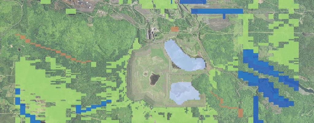
88 Bear Creek Barr Footer: ArcGIS , :31 File: I:\Client\PolyMet_Mining\Work_Orders\Agency_Preferred_Alternative\Maps\Support_Document\Water\Water_Modeling_Package\Plant_Site\MODFLOW_Model_Document\Large Figure 5 Model Boundary Conditions Layers 1 & 2.mxd User: arm2 First Creek Project Areas Stephen s Cr ek Heikkil la River Cells (Wetlands) - Layer 2 Drain Cells - Layer 2 Constant-Head Cells - Layer 2 Constant-Head Cells - Layer 1 Creek Second Creek Embarrass River Unnamed Creek Partridge River Model Extent Model Grid Trimble Creek Unnamed Creek Camp Eight Creek Former Channel Mud Lake Creek Partridge River I Former Channel Miles Wyman Creek Spring Mine Creek Ridge Creek Longnose Creek Image Source: FSA, Large Figure 5 MODEL BOUNDARY CONDITIONS LAYERS 1 AND 2 NorthMet Project Poly Met Mining, Inc.

89 Bear Creek Barr Footer: ArcGIS , :44 File: I:\Client\PolyMet_Mining\Work_Orders\Agency_Preferred_Alternative\Maps\Support_Document\Water\Water_Modeling_Package\Plant_Site\MODFLOW_Model_Document\Large Figure 6 Hydraulic Conductivity Zones in Layer 1.mxd User: arm2 First Creek Stephen s Cr ek Heikkil Cell 1E LTVSMC Fine Tailings Cell 1E LTVSMC Coarse Cell 2E LTVSMC Fine Tailings Cell 2E LTVSMC Fine Tailings Cell 2W LTVSMC Fine Tailings Cell 2W LTVSMC Coarse la Creek Second Creek Embarrass River Unnamed Creek Partridge River Model Extent Model Grid Trimble Creek Unnamed Creek Camp Eight Creek Mud Lake Creek Partridge River I Miles Wyman Creek Spring Mine Creek Ridge Longnose Creek Creek Image Source: FSA, Partridge River Large Figure 6 HYDRAULIC CONDUCTIVITY ZONES IN LAYER 1 NorthMet Project Poly Met Mining, Inc.

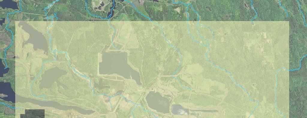
90 Bear Creek Barr Footer: ArcGIS , :05 File: I:\Client\PolyMet_Mining\Work_Orders\Agency_Preferred_Alternative\Maps\Support_Document\Water\Water_Modeling_Package\Plant_Site\MODFLOW_Model_Document\Large Figure 7 Hydraulic Conductivity Zones in Layer 2.mxd User: arm2 First Creek Stephen s Cr ek Heikkil Unconsolidated Deposits Bedrock Hydraulic Conductivity Zone la Creek Second Creek Embarrass River Unnamed Creek Partridge River Trimble Creek Unnamed I Creek Camp Eight Creek Mud Lake Creek Partridge River Miles Wyman Creek Spring Mine Creek Ridge Longnose Creek Creek Image Source: FSA, Partridge River Large Figure 7 HYDRAULIC CONDUCTIVITY ZONES IN LAYER 2 NorthMet Project Poly Met Mining, Inc.

91 Barr Footer: ArcGIS , :04 File: I:\Client\PolyMet_Mining\Work_Orders\Agency_Preferred_Alternative\Maps\Support_Document\Water\Water_Modeling_Package\Plant_Site\MODFLOW_Model_Document\Large Figure 8 Recharge Zone Extents First Active Layer.mxd User: mjw Imagery: FSA, Unconsolidated Deposits Cell 1E and 2E Ponds Cell 2W LTVSMC Coarse Tailings Cell 2W LTVSMC Fine Tailings Bedrock Model Extent Model Grid I Miles Large Figure 8 RECHARGE ZONE EXTENTS FIRST ACTIVE LAYER NorthMet Project Poly Met Mining, Inc.

92 Barr Footer: ArcGIS , :19 File: I:\Client\PolyMet_Mining\Work_Orders\Agency_Preferred_Alternative\Maps\Support_Document\Water\Water_Modeling_Package\Plant_Site\MODFLOW_Model_Document\Large Figure 9 Calibration Observation Locations.mxd User: mjw River Cells Drain Cells CP1!( GW015!< CP12!( Bedrock Hydraulic Conductivity Zone Control Point GW014 CP14!( CP9!( GW002!< CP13!( CP17!( CP2!( GW009!< GW010 P2HA-99 GW011!< GW013 P3H-99!<!< DH96-28 GW012 P2HB-99 DH96-37 P1H1-99 PN1J-99!< P3H1-99!<!<!(!<!<!<!<!( GW001 GW006 P2H1-99!<!<!<!< F-2!< P1H-99 A-3 DH96-32 Cell 2E!< A-9!< DNR-1!< DH96-30 GW007 DNR-5!< CP6 DNR-2!<!<!( DNR-6 D-1 CP8 DNR-4!<!<!< D-4!( GW005!< DNR-3a Cell 1E E-5!<!<!<!<!< GW008 GW003 DNR-3 CP10!<!(!<!<!< CP11 GW004!( DH96-11 DH96-10!( Drawdown Observation I < Transient Head Observation Steady-State Head!<( Observation Model Extent Model Grid Miles CP3!( CP16!( CP5!( CP7!( CP4!( CP15!( Imagery: FSA, Large Figure 9 CALIBRATION OBSERVATION LOCATIONS NorthMet Project Poly Met Mining, Inc.

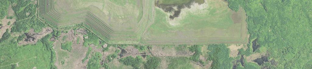
93 Barr Footer: ArcGIS , :11 File: I:\Client\PolyMet_Mining\Work_Orders\Agency_Preferred_Alternative\Maps\Support_Document\Water\Water_Modeling_Package\Plant_Site\MODFLOW_Model_Document\Large Figure 10 Simulated Groundwater Head Contours and Head Residuals in Layer.mxd User: kam2!.!. 1520' 1540' 1550' 1570' A-3-9.2!. A !. DH ' E-5-4.6!.!.!. 1530'!. GW !.!.!. DH Steady-State Head Observations with Negative Head Residuals in Feet 1590' DNR ' Steady-State Head Observations with Positive Head Residuals in Feet Simulated Groundwater Contours (ft) P1H ' 1580' GW !. GW P2HA-99 DH P1H !.!.!.!.!.!.!. DH DH DNR-4 5.3!. DNR !. DNR DNR-3a DNR !.!. 1660' 1650' 1640' 1650' 1620' 1650' I 1630' 1580' PN1J DNR ' F-2-5.8!.!.!.!. 1630' 1610' Cell 2E ' 1510' 1600'!. Cell 1E Miles D !. D ' 1660' 1510' 1640' 1650' 1640' 1660' 1640' Large Figure 10 SIMULATED GROUNDWATER HEAD CONTOURS AND HEAD RESIDUALS MODEL LAYER 1 NorthMet Project Poly Met Mining, Inc. 1650' Imagery: FSA, 2013.

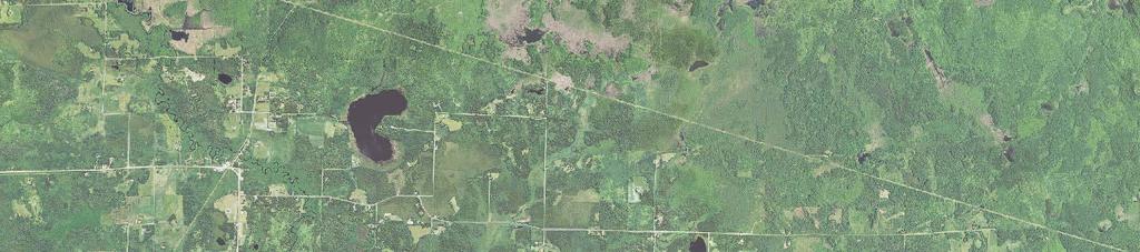
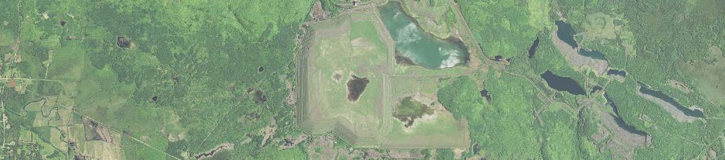
94 1430' Barr Footer: ArcGIS , :07 File: I:\Client\PolyMet_Mining\Work_Orders\Agency_Preferred_Alternative\Maps\Support_Document\Water\Water_Modeling_Package\Plant_Site\MODFLOW_Model_Document\Large Figure 11 Simulated Groundwater Head Contours and Head Residuals in Layer 2.mxd User: kam2!.!. 1430' 1500' 1640' 1410' 1570' 1460' 1440' 1750' 1470' 1420' 1470' 1620' 1520' 1460' 1490' Steady-State Head Observation with Negative Head Residual in Feet GW !. 1730' Steady-State Head Observation with Positive Head Residual in Feet Simulated Groundwater Contours (ft) Model Extent Model Grid 1480' A GW007!. 9.3!. 1520' 1490' 1430' 1480'!. 1660' 1550' 1510' B-2 3.2!. GW !. 1490' 1460' GW ' 1530' 1470' 1510' 1500' 1450' 1490' 1570' 1590' I Miles GW !. G-2! ' 1580' 1490' 1580' 1560' 1670' 1510' 1560' 1500' 1600' 1540' 1560' 1610' 1440' 1530' 1630' 1620' 1440' 1530' 1680' 1650' 1540' Imagery: FSA, Large Figure 11 SIMULATED GROUNDWATER HEAD CONTOURS AND HEAD RESIDUALS MODEL LAYER 2 NorthMet Project Poly Met Mining, Inc.

95

96

97

98

99

100

101

102 Barr Footer: ArcGIS , :08 File: I:\Client\PolyMet_Mining\Work_Orders\Agency_Preferred_Alternative\Maps\Support_Document\Water\Water_Modeling_Package\Plant_Site\MODFLOW_Model_Document\Large Figure 19 Flotation Tailings Basin Configuration Mine Year1.mxd User: mjw Dam Beach Pond CELL 2W I CELL 2E CELL 1E Miles Image Source: FSA, Large Figure 19 FLOTATION TAILINGS BASIN CONFIGURATION - MINE YEAR 1 NorthMet Project Poly Met Mining, Inc.

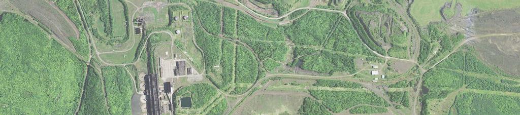
103 Barr Footer: ArcGIS , :02 File: I:\Client\PolyMet_Mining\Work_Orders\Agency_Preferred_Alternative\Maps\Support_Document\Water\Water_Modeling_Package\Plant_Site\MODFLOW_Model_Document\Large Figure 20 Flotation Tailings Basin Configuration Mine Year7.mxd User: kam2 Dam Beach Pond CELL 2W CELL 2E CELL 1E I Miles Image Source: FSA, Large Figure 20 FLOTATION TAILINGS BASIN CONFIGURATION - MINE YEAR 7 NorthMet Project Poly Met Mining, Inc.

104 Barr Footer: ArcGIS , :25 File: I:\Client\PolyMet_Mining\Work_Orders\Agency_Preferred_Alternative\Maps\Support_Document\Water\Water_Modeling_Package\Plant_Site\MODFLOW_Model_Document\Large Figure 21 Flotation Tailings Basin Configuration Mine Year8.mxd User: mjw CELL 2W CELL 1E/2E Image Source: FSA, Dam Beach Pond I Miles Large Figure 21 FLOTATION TAILINGS BASIN CONFIGURATION - MINE YEAR 8 NorthMet Project Poly Met Mining, Inc.

105 Barr Footer: ArcGIS , :02 File: I:\Client\PolyMet_Mining\Work_Orders\Agency_Preferred_Alternative\Maps\Support_Document\Water\Water_Modeling_Package\Plant_Site\MODFLOW_Model_Document\Large Figure 22 Flotation Tailings Basin Configuration Mine Years and Long-term Closure.mxd User: mjw CELL 2W CELL 1E/2E Image Source: FSA, Dam Beach Pond I Miles Large Figure 22 FLOTATION TAILINGS BASIN CONFIGURATION - MINE YEARS 18, 20 AND LONG-TERM CLOSURE NorthMet Project Poly Met Mining, Inc.

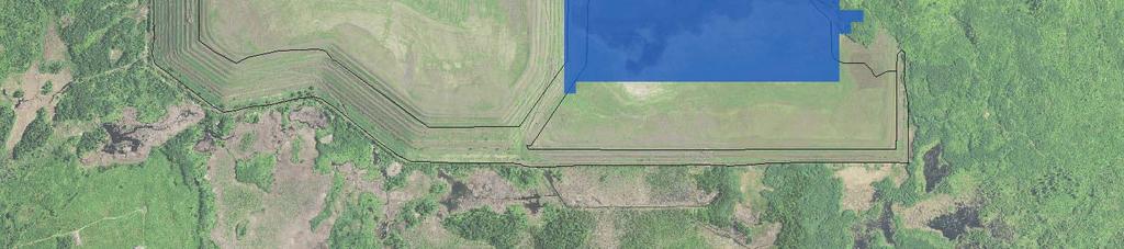
106 Barr Footer: ArcGIS , :58 File: I:\Client\PolyMet_Mining\Work_Orders\Agency_Preferred_Alternative\Maps\Support_Document\Water\Water_Modeling_Package\Plant_Site\MODFLOW_Model_Document\Large Figure 23 Layer 1 Boundary Conditions - Mine Year 1.mxd User: kam2 Project Areas Specified-Head Cells LTVSMC Tailings Basin DNR Mine Features, 2011 I Miles Image Source: FSA, Large Figure 23 MINE YEAR 1 BOUNDARY CONDITIONS - LAYER 1 NorthMet Project Poly Met Mining, Inc.

107 Barr Footer: ArcGIS , :53 File: I:\Client\PolyMet_Mining\Work_Orders\Agency_Preferred_Alternative\Maps\Support_Document\Water\Water_Modeling_Package\Plant_Site\MODFLOW_Model_Document\Large Figure 24 Layer 1 Boundary Conditions - Mine Year 7.mxd User: kam2 Project Areas Specified-Head Cells LTVSMC Tailings Basin DNR Mine Features, 2011 I Miles Image Source: FSA, Large Figure 24 MINE YEAR 7 BOUNDARY CONDITIONS - LAYER 1 NorthMet Project Poly Met Mining, Inc.

108 Barr Footer: ArcGIS , :44 File: I:\Client\PolyMet_Mining\Work_Orders\Agency_Preferred_Alternative\Maps\Support_Document\Water\Water_Modeling_Package\Plant_Site\MODFLOW_Model_Document\Large Figure 25 Layer 1 Boundary Conditions - Mine Year 8.mxd User: kam2 Project Areas Specified-Head Cells LTVSMC Tailings Basin DNR Mine Features, 2011 I Miles Imagery: FSA, Large Figure 25 MINE YEAR 8 BOUNDARY CONDITIONS - LAYER 1 NorthMet Project Poly Met Mining, Inc.

109 Barr Footer: ArcGIS , :47 File: I:\Client\PolyMet_Mining\Work_Orders\Agency_Preferred_Alternative\Maps\Support_Document\Water\Water_Modeling_Package\Plant_Site\MODFLOW_Model_Document\Large Figure 26 Layer 1 Boundary Conditions - Long-term Closure.mxd User: kam2 Head-Dependent Boundary Cells LTVSMC Tailings Basin DNR Mine Features, 2011 I Miles Imagery: FSA, Large Figure 26 LONG-TERM CLOSURE BOUNDARY CONDITIONS - LAYER 1 NorthMet Project Poly Met Mining, Inc.

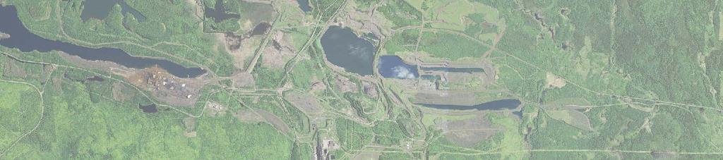
110 Barr Footer: ArcGIS , :33 File: I:\Client\PolyMet_Mining\Work_Orders\Agency_Preferred_Alternative\Maps\Support_Document\Water\Water_Modeling_Package\Plant_Site\MODFLOW_Model_Document\Large Figure 27 Bottom Layer Boundary Conditions.mxd User: kam2 Seepage Barrier Constant Head Cells River Cells (Wetlands) Drain Cells Model Extent Model Grid I Miles Large Figure 27 BOTTOM LAYER BOUNDARY CONDITIONS - PREDICTIVE SIMULATIONS NorthMet Project Poly Met Mining, Inc.