Reconstruction of Glacier Mass Balance and Sensitivity Tests to Climate Change: A case study of Ålfotbreen and Nigardsbreen

Transcription

1 Reconstruction of Glacier Mass Balance and Sensitivity Tests to Climate Change: A case study of Ålfotbreen and Nigardsbreen Master Thesis in Meteorology Wangdui December 2011 UNIVERSITY OF BERGEN GEOPHYSICAL INSTITUTE

2 The picture on the front page shows historical front positions of the Nigardsbreen glacier identified by glacier moraines, with the characters from 1748, 1850 and (Photo Bjørn Wold 1990). The picture taken from:

3 Acknowledgements My deepest gratitude goes to my supervisor, Professor Asgeir Sorteberg, for his guidance, patient, critical comments and many useful suggestions throughout this work. Moreover, his assistance on MATLAB program and detailed writing corrections were very helpful. All his kind help has made me to achieve this thesis. I would like to express my heartfelt gratitude to Professor Y. Gjessing, who initially helped me to obtain this opportunity to study in Norway and had taught me a special course on glaciology at beginning of my master study. I am also very grateful to his continuous encouragement both in my study and life; and his constantly concerning about all Tibetan students in Bergen that made our study and life become easier. I m very grateful to Norwegian Quota program for financial support during my master study. I m also grateful to Network for University Co-operation Tibet-Norway for providing me this opportunity to study in Norway, and their financial support and had helped me to improve my English in many ways in the past years. And also great thanks to Tibet University supported me to take master study in Norway. Thanks to Dr. Caidong for his help to get this opportunity and have taken me for field-work on glacier in Tibet. Thanks to all of Tibetan students for many unforgettable memory in Norway. Thanks to my fellow students and friends created a favorable study environment at Geophysical Institute. Finally I would like to thanks to my wife Lhazhen for her encouragement and take care of our daughter in this period. And also thanks my mother in law who was taking care of my daughter. Wangdui

4

5 Abstract A physically-based one dimensional CROCUS snow model was applied to simulate the surface mass balances of Ålfotbreen ( ) and Nigardsbreen ( ) in southern Norway. The required hourly meteorological input data (9 parameters) are obtained from daily data of meteorological observation from stations surrounding the glaciers combined with NCEP 6 hourly reanalysis data to get the diurnal cycle. The results of simulations show that the model was able to simulate the mass balance of Ålfotbreen Nigardsbreen. The correlation coefficients were 0.99 and 0.97 for cumulative mass balance and 0.89 and 0.76 for net balance compared to the observations, respectively. Mass balances for long-term trends are also investigated. According to the model, precipitation changes dominated the contribution of the mass balances changes from the beginning of simulation (1960s) to 1995 for both glaciers. In the last 15 years ( ), temperature changes was the major contributor of mass balance changes for Ålfotbreen, but precipitation was still the major contributor to the changes in cumulative mass balance for Nigardsbreen. The average mass balance sensitivities to temperature were -0.76m w.e./1k and -0.35m w.e./k and to precipitation were 0.33m w.e./10% and 0.18m w.e./10% for Ålfotbreen and Nigardsbreen, respectively. The results of mass balance sensitivity tests indicate that Ålfotbreen is more sensitive to both temperature and precipitation change than Nigardsbreen. Our results also indicate a nonlinear relation between net mass balance sensitivity and temperature perturbation for both glaciers, but no significant non-linearity were found for different precipitation perturbations.

6

7 CONTENTS Chapter 1 Introduction 1 Chapter 2 Energy and mass budget on a glacier surface General review of glaciology Surface energy budget Net radiation Shortwave radiation Long-wave radiation Turbulent fluxes Surface mass budget Surface accumulation Surface ablation Annual (net) mass balance and seasonal cycle Annual glacier balance and average specific balances Chapter 3 CROCUS snow model Description Input and output Files The MET file The PROi file The PARAM file The GEO file The PROo file The QOUT file The TSURF file The FLUX file Chapter 4 Data and method CROCUS input data The initial snow profile (The PROi file) The geographical characteristics (The GEO file) Hourly meteorological input data (The MET file) Preprocessing of meteorological data Correction of data from nearby meteorological stations to the glacier elevation... 26

8 Meteorological stations used to approximate conditions on the glaciers Data for Ålfotbreen glacier Glacier observations Meteorological model input Data for Nigardsbreen glacier Glacier observations Meteorological model input Processing of model output Chapter 5 Model results and analysis Simulations for Ålfotbreen Model tuning Long-term trends in mass balance Net mass balance Cumulative mass balance Sensitivity test Sensitivity to temperature Sensitivity to precipitation Sensitivity to snow surface albedo Sensitivity to temperature lapse rate and to the vertical precipitation gradient Simulation for Nigardsbreen Model tuning Long-term trends in mass balance Net mass balance Cumulative mass balance Sensitivity test Chapter 6 Conclusions 58 Appendix A Appendix B Appendix C Appendix D Appendix E Appendix F Appendix G References... 81

9 Chapter 1 Introduction The glacier mass balance forms a vital link between the changing atmospheric environment and glacier dynamics and hydrology (Braithwaite, 2002). On the west coast of Norway the glacier mass balance is governed by synoptic scale meteorological processes making the glaciers interesting historical archives of synoptic scale changes in precipitation and temperature. Glacier melt is also an important water resource that feeds hydroelectric power stations or irrigation systems. Another important parameter in glacier research is the equilibrium line altitude (ELA). The ELA is regarded as a useful parameter to quantify the effect of climatic variability on a glacier (Lie and Nesje, 2003) and it is widely used to infer the present and past climatic conditions. Glaciers cover about 1% of the land area in Norway, and many of them are situated in region with considerable hydropower potential (Andreassen, 2005). Detailed mass balance investigations were started in the 1960s at selected glaciers by Norwegian Water Resources and Energy Directorate (NVE), mainly for hydrologic purpose and results from NVE s glaciological investigations have been published annually or biannually since 1963 (Andreassen, 2005). Traditionally glaciological, hydrological and mapping (geodetic) methods are most often used to measure the glacier mass balance (Tangborn, 1975). The conventional method of glaciers mass balance is the glaciological method, which is with stakes and snow pits, but it is a laborious way of doing long-term measuring of glacier changes. In addition, the method may be difficult to perform due to difficult access to remote and high cliffy mountainous glaciers (Braithwaite, 2002). Modeling of glacier mass balance has often been done using so called degree-days model which uses air temperature and precipitation as meteorological input parameters. More 1

10 sophisticated models calculating the energy budget also exist and mass balance modeling is a crucial step in modeling the response of glacier to future climate change (Hock 2007). In this thesis, we applied the CROCUS snow model which has a full energy budget and treatment of snow metamorphosis in up to 50 layers to simulate the mass balances of Ålfotbreen (period ) and Nigardsbreen (period ) in south-western Norway. In the thesis we investigate the causes of the observed balance long-term trends in mass balance and tested the mass balance sensitivities to several climatic parameters (temperature, precipitation, snow surface albedo, temperature lapse rate and vertical precipitation gradient), sensitivities of the equilibrium line altitude (ELA) to temperature and precipitation are also tested for Nigarsbreen. The physically based CROCUS model requires hourly meteorological parameters as input data. The hourly data (temperature, precipitation, wind speed, relative humidity, and cloud cover) are obtained from daily data of meteorological observation from stations surrounding the glaciers combined with 6 hourly NCEP reanalysis data to get the diurnal cycle and modeled hourly shortwave radiation (direct and scattered incoming solar radiations), long-wave radiation and precipitation type. (the location of the glaciers and chosen stations seen in map Appendix F). Tuning of the model are carried against the mean mass balance from NVE s glaciological investigations report 2009 which have 46 and 48 years of mass balance observations for Ålfotbreen and Nigardsbreen, respectively. Ålfotbreen (ELA 1200) is both the westernmost and the most maritime glacier in Norway and is located in Sogn and Fjordane County close to the coast. It is subject to very maritime conditions with extremely high annual precipitation. Nigarbreen (E 1500) is one of the largest and best known outlet glaciers from Jostedalsbreen, the largest ice cap in Europe. Nigardsbreen is situated in Sogn and Fjordane County and has an area of 47.2 km 2 (measured in 2009) and flows to the south-east. The main purpose of this thesis is: 1. Reconstruct the mass balances (the net balance and cumulative balance) of Ålfotbreen and Nigardsbreen during the period and , respectively, using meteorological data from nearby stations. 2

11 2. Quantify the contribution of temperature and precipitation variations on the long-term mass balance trend. 3. Test the sensitivities of the mass balances and ELA to several meteorological parameters (as mentioned above). 3

12 Chapter 2 Energy and mass budget on a glacier surface 2.1 General review of glaciology Glacier mass balance studies are concerned with change in glacier mass and distribution of this change in space and time (Paterson, 1994). Glaciers usually gain mass (accumulation) in winter season by precipitation (snow fall) and loss mass (ablation) in summer season by melting, sublimation and ice calving, these are called winter balance and summer balance, respectively. The different between the accumulation and the ablation is referred to as the net balance over the balance year. Usually, the balance year is the period between two successive summer minimums. Paterson (1994) mentions that often the balance year is defined by an observational period (close to fixed calendar dates). If accumulation exceeds ablation in a particular year the glacier has a positive mass balance, while a negative mass balance is resulting from ablation exceeding the accumulation. Most of glaciers have an accumulation zone (Figure 2.1) at higher altitude where they gain mass and ablation zone at low altitude where they loss mass. The boundary between these two zones is the equilibrium-line, at an altitude called the equilibrium line altitude (ELA), where the amount of mass gain and loss just balance (net balance is zero). The ELA is a theoretical line but is a useful parameter to indicate influence of climatic variability on a glacier and it is widely used to infer the climate condition in present and past (Lie, et. al., 2003). Usually the ELA will vary not only from year to year on the same glacier but also varies between glaciers that are situated in the same region. If the ELA is constant for longer period, then we say the glacier is at steady state. Although the changes in glaciers mass balance are contributed by many climatic parameters and the relations are complicated, numerous papers indicate that temperature and precipitation (snowfall) are the most important contributors to mass balance and ELA variability for most of glaciers. 4

13 Figure 2.1: Zones in accumulation area. Taken from Paterson (1994). 2.2 Surface energy budget Most of this section is taken from Cuffey and Paterson (2008). Glacier melt and temperature variation are determined by the energy budget (or balance) at the glacier-atmosphere interface, which is controlled by the meteorological conditions above the glacier and physical properties of glacier itself. Hence it partly determines the glacier mass balance and in turn the glacier can modify its own local climate. The energy exchange mainly take place in a thin layer at the surface (snowpack or glacier ice), as seen in Figure 2.2, and involves solar radiation, long-wave radiation, sensible and latent heat turbulent fluxes, ground heat flux as well as the energy flux carried by precipitation. The energy exchange surplus or deficit depends on the prevailing climatic conditions. A physically based energy balance can derived at any point on the surface at any instant. If we are not taking into account horizontal transfer of heat the surface energy flux E N (unit Wm -2 ) can be written as E N E S E S E L E L E G E H E E E P (2.1) Where ES and ES are incoming and reflected solar radiation (shortwave radiation), EL are incoming and outgoing long-wave radiation, and E G is the subsurface energy flux, EL and EH 5

14 and E are the turbulent fluxes of sensible and latent heat, E EP is heat flux from precipitation, which is negligible when the surface is melting but may be significant if the rain can freeze. The immediate positive net energy (gain energy) used to melt snow and ice, if melt water refreeze in the snowpack this term is negative (loss energy). Figure 2.2: Energy balance for an open snow pack. Taken from Armstrong and Brun (2008) Net radiation The net input of all radiative energy to the surface is the sum of net shortwave and long-wave radiation. Shortwave radiation (solar radiation) originates directly from the sun and most of solar energy lies in wavelengths ranging approximately from 0.15 to 4μm, and long-wave radiation (terrestrial radiation) which is thermal radiation originating from the surface or atmosphere in wavelength ranging from 4 to 120μm. There is little overlap between the spectra of solar and terrestrial radiation. The net radiation can be written as or E E E E E (2.2) R S s S L L L E E ( 1 ) E E (2.3) N L 6

15 Here E is rate of incoming solar radiation which is sum of direct, scattered and reflected from s surrounding terrain radiation, is surface albedo. Thus E ( 1 ) represent the net shortwave radiation that surface received solar radiation, and the sum of last two terms is net long-wave radiation. s Shortwave radiation Entering normally on the top of the atmosphere, the energy flux of solar radiation is approximately 1368Wm 2, called the solar constant. As it travels through the atmosphere, it is partitioned into direct and diffuse components. This is mainly due to the fact that solar radiation is partly scattered and absorbed by air gases, water droplets, ice crystals, and liquid and solid particles, all are processes having different wavelength dependencies. The total solar flux reaching the surface is called the insolation or the global radiation. Beside the atmosphere conditions and cloud, the characteristic of the site surrounding terrain is crucial for the total radiation in complex topography. Thus the global radiation is constitutes of three components: the direct solar radiation, the diffuse solar radiation coming from all directions in the sky and reflected solar radiation from surrounding terrain. The direct downward solar radiation that reaching at horizontal surface E is that: Sd E E cos(z ) Sd So with P /( Po cosz ) (2.4) o Where E So is solar constant, and Z is the zenith angel, it varies with latitude ( ), time of year, and time of day: cos Z sin sin cos cos cosh (2.5) Where is solar declination, the angular between the sun and the equator, h is the hour angel, varies with the time of the day, h 0 at local noon. The parameter is the atmospheric transmissivity, value less than one. At sea level, its value about 0.84 for a clear sky and 0.6 for thick haze. decreases to zero under heavy cloud cover, in which case only diffuse and o o 7

16 reflected radiations contribute to insolation. P is the atmospheric pressure and P o is mean atmospheric pressure at sea level. The direct radiation on a glacier surface increases with altitude, because the thickness of atmosphere traversed by the solar beam decrease. The amount of diffuse solar radiation depends on atmosphere conditions. Diffuse radiation reaching the surface consists of radiation that is initially scattered from the sky and backscattered radiation that is reflected by the snow surface and subsequently redirected downward by scattering in the atmosphere Long-wave radiation Long-wave outgoing radiation E, is referring to the radiation emitted by and reflected from L the surface. Snow, ice and liquid water behaves as near-perfect black body in the infrared wavelength radiation, emitted flux depend only on its temperature, calculated by the Stefan- Boltzmann Law E L T S 4 S (2.6) Where T is the surface temperature and the negative sign indicates a loss of energy from the S surface. is Stefan-Boltzmann constant, has value of K. S is surface emissivity, typical value for snow, ice and liquid water. S Long-wave incoming radiation E, results from emission by clouds and by atmospheric water L vapor, carbon dioxide, and ozone. Radiation is continually being absorbed and emitted at different levels in the atmosphere. The total flux of reaching to the surface varies largely due to variation in cloudiness, temperature and water vapor contain in the atmosphere. The information of these varies are seldom available and E must be measured or parameterized at L a site, thus E is difficult to predict. Most parameterizations define as effective atmospheric L emissivity a and near-surface air temperature Ta such that E L T a 4 a (2.7) 8

17 The air temperature used is usually at 2m above the surface. Most calculate a in terms of humidity and air temperature measured at 2m above the surface. In cloudy skies, and can be less than 0.5 for clear skies, a typical value 0. 8 for a late-summer average. a a Turbulent fluxes Part of the below text is taken from Hock (2005). Turbulent eddies mix the air vertically and transfer the heat to or from the surface by turbulent fluxes of sensible heat and latent heat. They are driven by the temperature and moisture gradients between the air and the surface and by turbulence in the lower atmosphere. The vertical fluxes of heat are obtained from Flux-gradient Theory as E E H E T acak H (2.8) z q alv K E (2.9) z Where E and E are the sensible heat and latent heat, respectively. H E a is air density, ca is the specific heat capacity of air, L is the latent heat of evaporation, z is the height above the v surface, K and K E are known as the eddy diffusivity for heat and water vapor exchange. H and K specify the effectiveness of the transfer process and depend on wind speed, surface E roughness and atmosphere stability. K H The Flux-gradient method involves measurement of temperature, humidity and wind speed at preferably more than two levels within the first few meters above the surface. Since detailed profile measurements are seldom available, a bulk aerodynamic method is frequently used for practical purposes. Integrating equation (2.8) and (2.9), the bulk aerodynamic can be written as E H a a H a S c C u T T (2.10) E E a v E a S L C u q q (2.11) 9

18 Where u is mean wind speed, and C andc are the bulk exchange coefficients for heat and H E moisture. Ta andt S are the stand for temperature of the lower boundary layer and the surface, and qa and q are the corresponding specific humidities. For a melting surface ( S T S 0 C, e es 6. 11hpa ), the sensible E H and latent heat E can be calculated from only one level of measurement. E 2.3 Surface mass budget The surface mass balance or mass balance budget is dealing with changes in the mass of a glacier and the distribution of these changes in space and time. Mass exchanges at the surface dominate the budget of most glaciers and contributions from the several processes determine the surface balance rate at a point: b s a a m a s a (2.12) s a s r w Representing snowfall ( a s ), avalanche deposition ( a a ), melt ( m s ), refreezing of water ( a r ), sublimation ( s ), and wind deposition ( a ), the dot above variables denote the rate of change w of mass with time. Sublimation can be either positive or negative, usually glacier loss mass by sublimation exceed the gains from vapor deposition. Wind deposition can also be either positive or negative. Refreezing of water refers mostly to melt-water, but rain and runoff from adjacent hill slopes can also freeze. At many glaciers, snow fall and melt dominate the surface balance Surface accumulation Most of the information in this section is found in Hock (2010). Accumulation is all processes that add mass to the surface of glacier. Components: Snow fall (usually the most important). 10

19 Deposition (freezing rain and solid precipitation other forms than snow contribute to the accumulation; direct deposition of atmospheric water vapor and supercooled droplets produce frost and rime, respectively; these are usually negligible accumulation processes) Redistribution by wind and avalanching (accumulation may differ from snowfall because winds carry snow along the surface; can be important for the survival of, for example, small cirque glaciers), avalanching of snow from steep valley slopes and cirque headwalls is an important source of accumulation for some mountain glaciers) Refreezing of meltwater (refreezing of melt forms superimposed ice on the surface or ice layer in the firn; negligible refreezing occurs in ablation zones, because meltwater drains easily) Surface ablation Most of the information in this section is found in Hock (2010). Ablation is all processes that reduce the surface mass of the glacier. (A glacier surface ablates mostly by melt and sublimation) Components: Melting (usually the most important on land-based glacier, refreezing of meltwater is not referred to as ablation; if the temperature of the snow/ice surface is at melting point, the rate of melt increases in proportion to the net energy flux) Sublimation (occurs at all temperature and is the dominant ablation mechanism in very cold environment where surface temperature seldom reach melting point even in summer) Calving (is iceberg discharge into seas or lake; important, for example, in Greenland and Antarctic, where approximately 50% and 90%, respectively, of all ablation occurs via caving) Avalanching Loss of windborne blowing snow and drifting 11

20 2.3.3 Annual (net) mass balance and seasonal cycle Some of the information in this section is from Hock (2010). The surface balance rate varies over hours and weeks and the variability is smaller for longer periods such as months or seasons. Mass balance at the end of balance year is called the annual mass balance (or net mass balance) at a point ( b n ). It is the sum of mass balance rate ( b s, as seen in section 2.3) over the balance year, b b n dt (2.13) It can also be described as the sum of the winter balance ( b w ) and summer balance ( b s ), s b n bw bs (2.14) The surface balance varies considerably over the season, dominated by accumulation in winter and ablation in summer. At mid-latitude, there are distinctly difference accumulation and ablation seasons. Figure 2.3 depicts an idealized seasonal cycle. Mass balance per unit area is defined as specific mass balance, The prefix specific is not necessary in general. Figure 2.3: Variation of accumulation, ablation, and mass balance during a glaciological year. Taken from Hock (2010). 12

21 2.3.4 Annual glacier balance and average specific balances Integrating the annual specific balance over the total area of glacier, A, gives the net balance of the whole glacier for one year, B : n Bn bnda and bn Bn / A (2.15) b is defined as average specific balance, also called the average net balance. This quantifies n the mass per unit area or equivalent thickness of ice or water. 13

22 Chapter 3 CROCUS snow model 3.1 Description The CROCUS model was initially developed by Météo-France for simulation of Alpine snow and operational avalanche forecasting. The model code has been improved several times. And in this thesis we use version 2.4 which uses International System unites and is coded in the FORTRAN90 language. CROCUS has been applied to various scientific problems outside its originally planned domain of application (Gerbaux and others, 2005). CROCUS is a physically based one-dimensional snow model, in which the snow depth can be divided into maximum 50 layers parallel to the ground. The surface energy and mass budgets are explicitly calculated at 10 minutes time steps using hourly meteorological conditions as input data (A schematic of N layer scheme for CROCUS is shown in Figure 3.1). It computes the evolution of snow temperature, density, liquid water content and grain type in each layer. The model simulates the heat conduction, melting/refreezing of snow layers, settlement, metamorphism, and percolation. A strength of the model is the detailed description of metamorphism process for different type of snow taking into account the size and shape of the snow grain which allows for a more accurate calculation of the albedo of the snow cover. The main techniques (representation of grain, principle, physical process and splitting and aggregation of layers) of the CROCUS model are seen in Appendix A - D. 3.2 Input and output files Most of the information found in this chapter is taken from Willemet (2008). 14

23 The required input data are the initial snow profile (PROi file) and series of hourly value of meteorological parameters (MET file), combined with name list file containing model parameters such as time step, parameterization switches and constants (PARAM), a geographical characteristic file (GEO) and outputs several files. Figure 3.1: Schematic diagram of the N layers scheme MET file hourlymet.data PROifile initial profile PARAM file name list GEO file geo.characteristic CROCUS PROofile simulatedprofile QUOT file daily output TSURF file hourlydada FLUX file surfacefluxs Figure 3.2: Input and output files for CROCUS 15

24 3.2.1 The MET file The MET is hourly meteorological data (one record per hour), the file contains 9 variable listed below with their unit The PROi file CROCUS needs an initial snow profile at the beginning of the simulation. This must contain: 1. Total number of layers 2. In each layer Snow thickness (SDZ) Snow temperature (ST1) Density dry snow (SRO) Liquid water content (SCW) Grain type Dendricity (SGRAN1) Sphericity (SGRAN2) Age (MSDAST) History variable indicating if there were water of faceted crystals before (MSHIST) 16

25 If there is no snow on the ground, it can be set to zero. Then the file has just 2 lines, a date (start year, month, day, hour in UTC) and zeros (lines starting with # is not read). Example of PROi file (no snow on the ground) # INITIAL PROFILE WITH NO SNOW ON THE GROUND # If there is snow on ground, specified each layer according to appendix A. Example of PROi file (with snow on the ground) The PARAM file This file is the name-list file. The CROCUS model reads a name-list with important settings such as dates for running the model, time step, output frequency and constants in different physical parameterizations The GEO file This file contains geographical characteristics for the simulation. 17

26 Example for the Ålfotbreen site: _ values for the solar radiation masks... 0 _ Alternative method to provide geographical characteristics is to modify the name list NVGEO Example &NVGEO ZLATNAM=61.75, ZLONNAM=5.67, ZEXPONAM=0., ZALTINAM=1385., IINCLINAM=0, IMASQNAM=36*0 &END ; Latitude of the simulation area ; Longitude ; Aspect (between 0 and ), South=180, North=0 ; Altitude ; Slope in degrees (flat terrain=0) ; Masks for the solar radiation Masks for the solar radiation are given with a 10 o step (36 rose), the first value corresponds to degree in the North. If the input values are measured code 36*0. The masks are used when input data are measured on a flat terrain and the simulation is realized in uneven terrain. The file GEO contains the same information as the name-list NVGEO. If the CROCUS model find a file GEO, the name-list NVGEO will not be used, if this file does not exist, name-list NVGEO will provide the geographical characteristics The PROo file This file contains the simulated snow profile and has the same format as the PROi file (the initial snow profile file, see section 3.2.2). Usually, in the output PRO file, the initial profile is in the record 1, simulated profiles are in the others. 18

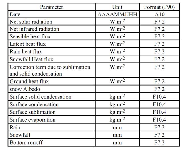
27 3.2.6 The QOUT files This is the daily output file. This output is validated by the logical variable LVQUOT in the namelist NVSIMU. Each day of the simulation, at a given hour (MHQ in the name-list NVSIMU), CROCUS writes a new record containing the following variables: The TSURF file This output file contains the surface temperature and is invoked by the logical variable LVSTS in the name-list NVSIMU. Each hour, CROCUS writes a new record containing the following variables: If there is no snow on the ground, is written. Logical LVNEWFMT (name-list NVSIMU) modifies the date format and insert a space between the variables The FLUX file This file contains for a given date the main fluxes during the past hour (LVFLUH=T) or day (LVFLUH=F) at the surface or at the bottom of the snow cover. Each line contains the following parameters: 19

28 20

29 Chapter 4 Data and method 4.1 CROCUS input data The one dimensional CROCUS model was used to performed simulations for a range of elevation points on a glacier surface. Glacier elevation points are distributed on the glacier surface from the start to the top of the glacier with equal vertical distance (altitude: dz). The schematic distribution of glacier surface elevation points can be seen Figure 4.1(a). As presented in section 3.2, CROCUS requires an initial snow profile (PROi file) and hourly meteorological data (MET file) as well as geographical characteristics (GEO file) and a name-list with parameter settings (PARAM file) as input data for each elevation points. (a) Figure 4.1: Schematic of glacier surface elevation points, elevation points are distributed on the glacier surface from glacier start to top of the glacier with equal-altitude, z, dz are point elevation and distance between adjacent elevation points in altitude, respectively. Dotted line means equivalent altitude on surface (a). Initial now profile with a given number of snow layers (b). 21 (b)

30 4.1.1 The initial snow profile (The PROi file) The model simulations start with snow cover on a glacier surface, initial snow and ice profile for each elevation point. As detailed observations of the snow and ice profile of the chosen glaciers do not exist for the initial profiles are made based on some simple assumptions. Assuming the initial surface snow profile looks like on Figure 4.1(b), snow layers are parallel to the ground with equal layer snow/ice depth in same elevation point. We divide the total snow and ice depth into 24 layers for Ålfotbreen and 35 layers for Nigardsbreen. The total depth in an elevation point depends on where on the glacier the point is. We assume the glacier to be thinnest at terminus and increasing linearly in depth to the top. The profile is made by assuming a terminus depth and a mean depth. The end depth is then calculated as: start_depth = terminus_depth + 2 (mean_depth terminus_depth) The total depth of each elevation point is calculated by linear interpolation between the start and terminus depth. As an example: suppose that total depth at terminus of the glacier is 10m (terminus_depth) and the glacier has a mean depth of 100m (mean_depth) in middle of the glacier, then the start depth (top of glacier) (start_depth) will be 190 m. The depth of each layer is calculated as the total depth divided by number of layers. Each layer needs a set of initial temperatures, density, snow grain size and the history of the grain formation. These values are not known and are set uniformly for all elevations and layers as below, Layer temperature (T): 0 Layer dry now density: 850g/cm -3 Layer liquid water density: 0 g/cm -3 Layer 1st grain: Layer 2nd grain: 3.00 Historical of snow layer: 0 An example of the PROi file is found in Figure

31 Figure 4.2: Example of PROi for Ålfotbreen, elevation no The geographical characteristics (The GEO file) The GEO files for each elevation are done in the same script of the PROi files. Each file contains the geographical characteristics of simulation: latitude and longitude in decimals, aspect (orientation of slope South=180, North=0), altitude (m) and surface slope in degree (flat=0). The values of all parameters are same for all elevation points except for altitude which varies according to the distance from the glacier terminus. The model provides a possibility to apply a solar radiation masks (no mask=0) to simulate shadow effects of nearby mountains, but this has not been used Hourly meteorological input data (The MET file) Preprocessing of meteorological data Since only daily meteorological data are available from observations and the model requires hourly input the observed daily data was refined using other data sources. To get the daily cycle 23

32 we used NCEP 6 hourly reanalysis data which is available from 1948-present with a 2.5 *2.5 spatial resolution, by combining the daily meteorological observation with the 6 hourly reanalysis data we got the 6 hourly data that was interpolated to hourly values. This was done in a way that kept the observed daily values unchanged (the reanalysis was only used to calculate the 6 hourly deviations from the daily mean): x 6hourly = x obs daily + x reana 6hourly x reana daily (4.1) x hourly = x 6hourly after x 6hourly after t after t before t (4.2) This was done for temperature, precipitation, wind speed, relative humidity and cloud cover. When x is accumulated variable of precipitation, some additional conditions have to be met. For 6 hourly values, if there is precipitation both in observations and reanalysis the precipitation is divided throughout the day according to the when the reanalysis has precipitation. If there is precipitation in observations but not in reanalysis the precipitation is assumed to fall within 50% of the time. Conversely, if there is no precipitation in observations, but in reanalysis the precipitation is set to zero. For hourly values, since it is not usually raining a full 6 hour period the 6 hourly precipitation is assumed to fall within 50% of the time. Hourly direct and scattered incoming solar radiations (shortwave radiation) are calculated with geographical characteristic (latitude, longitude and elevation), precipitable water (from NCEP reanalysis), liquid water path (from NCEP reanalysis), fractional cloud cover (from observations), season, and time using SLOPERAD model based on Bird and Riordan (1986) for clear sky irradiance and corrections for clouds based on Stephens (1978). The model was provided by Asgeir Sorteberg. Incoming long-wave radiation is calculated with total cloud cover, near surface temperature (both from observations), and precipitable water (from NCEP reanalysis) based on Prata (1996) for clear sky and corrections for cloud follows Maykut and Church (1973), E clear = (1 1 + w (1 e w 12 ))σt 4 (4.3) 24

33 E cloud = ( G 2.75 ) E clear (4.4) where E clear and E cloud are the incoming long-wave radiation for clear sky and cloud cover, w is precipitable water, T is the air temperature at screen height, G is the cloudiness in tenths and σ is the Stefan-Boltzmann constant. Precipitation type (snow or rain) was calculated with the hourly precipitation and temperature data based on snow/rain function from Dai (2008), F = a tan b T s c d (4.5) F is the fraction of snow (in %) and a= , b=0.7205, c= and d= are parameters taken from Dai (2008). The process of making the hourly data is given in Table 4.1. Calculation of all hourly MET are developed in MATLAB by Asgeir Sorteberg. Table 4.1: The required hourly process Meteorological variable Temperature, Precipitation, wind speed, relative humidity, cloud cover Description Observed daily means, merged with 6 hourly reanalysis data using equation (4.1) and (4.2) Calculated based on input of observed cloud cover Shortwave radiation (direct and scattered incoming solar radiations ) Long-wave radiation Precipitation type and reanalysis data of precipitable water and liquid water path as well as latitude, longitude, elevation and time using the SLOPERAD model. Calculated based on the near surface temperature, precipitable water and total cloud cover (0-1) using equation (4.3) and (4.4) Calculated based on hourly precipitation and temperature data using equation (4.5) 25

34 Correction of data from nearby meteorological stations to the glacier elevation As the observed data are not available on the glaciers there is a need to correct the data for elevation difference between the meteorological stations used and the glacier. Temperature is elevation-corrected to take into account the difference in elevation from the station to the glacier terminus by assuming a constant temperature lapse rate (-0.65K/100m for Ålfotbreen and -0.75K/100m for Nigardsbreen) in addition the same lapse rate is used to calculate the temperature at different elevations on the glacier. The other parameters were assumed to be the same as for the nearby station (no corrections were done) Meteorological stations used to approximate conditions on the glaciers Hardly any single meteorological observation station near the glacier has sufficient data that cover the large time span we want to simulate ( for Ålfotbreen and for Nigardsbreen). Therefore merging of data from different stations was necessary to give a complete dataset. The method used to obtain observational estimates for the glacier is done in two steps: 1. Selection of main station 2. Merge of data from surrounding stations to get data for the full simulation period In the first step, a reference station is found by searching for a station as close as possible to the glacier and have recorded data covering at least half of the period of study. The database for finding the data was the Eklima( database, a web portal which gives free access to the meteorological data of the Norwegian Meteorological Institute. In the second step, once the reference station have been chosen, we have to find other stations that can be used to partly or completely fill the data gaps in the reference station. To do this we search for stations as close as possible to the reference station and with data for periods not covered by the reference station. In addition a period of data from both stations is needed to calculate a correction factor to merge the data. To find suitable stations to merge we considered the correlation between the reference station and the other station for the period 26

35 of overlapping data. Correlation coefficient was calculated after the removed seasonal cycles (refers to monthly mean values) in a pair of station. The seasonal cycle was removed because it tend affect the correlations and provide high correlations even for stations were the daily data did not correlate very well. Minimum correlation needed to keep the stations was set to 0.90 for temperature, 0.80 for precipitation, 0.50 for wind speed and 0.60 for humidity. This was subjectively chosen as a compromise to be able to fill in data for the whole period. If several stations fulfilled the criteria, the one closes to the reference station was chosen. Obviously it was not necessary to go to the second step if the reference station has a complete dataset for the whole period. In order to remove systematic differences between the reference station and the station selected for merging we bias correct the station selected for merging by using the period of overlapping data and calculating 36 ten-day mean deviations factors for the temperature corrections (equation 4.6) and ten-day mean multiply factors for the other parameters (equation 4.7). Then the corrected data values x are calculated as, _ corr station x corr _ station xstation xi, ref _ station xi, station (4.6) x corr_ station x station x x i, ref _ station i, station (4.7) Where station i station x is the observed data value for the station we want to correct, x and i, ref _ station x, is the ten-days mean value of the reference station data and corrective station data, respectively, and i is the ten-day averages throughout the year ( i 1,2,3,,36). For example: if there is overlapping data from , x and 1, ref _ station x, station 1 are the mean over all 1 st to 10 th of Januaries ). x _ is the corrected data that will be merged with the reference corr station station. An example of this process shown in Figure 4.3, in which a correction of precipitation data to reference station (Grøndlen) is made for simulation of Ålfotbreen via using 2 stations, Eikefjord (station A) and Eimhjellen (station B). 27

36 Figure 4.3: An example of process of merging station data, showing a correction of precipitation data to reference station (Grøndlen) for simulation of Ålfotbreen via using 2 stations, Eikefjord (station A) and Eimhjellen (station B). It is seen from the correction factor for station A that the correction is different in summer than winter. Emphasizing the need have different correction factors for different seasons. 4.2 Data for Ålfotbreen glacier Ålfotbreen (61 o 45 N, 5 o 40 E) has an area about 4.5km 2 (measured in 1997), located in western Norway close to the coast (35km). It is both the westernmost and the most maritime glacier in southern Norway and subject to a very maritime climate with extremely high precipitation (Oerlemans, 1992), According to Laumann and Reeh (1993) the precipitation in this region range from 3000mm to 5000mm, from sea level to the coastal mountains. Mass balance observations have been carried out by the Norwegian Water Resources and Energy Directorate (NVE) since 1963, a series of report Glaciological investigation in Norway published since

37 By the report 2009, Ålfotbreen has average winter balance of 3.73m w.e. and summer balance of -3.56m w.e. since1963. Ålfotbreen and its surrounding area is shown in Figure 4.4. Figure 4.4: Ålfotbreen and surrounding area, taken from NVE (2009) Glacier observations Based on the report of glaciological investigations in Norway 2009 by the Norwegian Water Resources and Energy Directorate (NVE, 2009), data for the equilibrium line altitude (ELA) and the total mass balance exist from 1963 to 2009 (47 years). Also glacier surface area at different elevations is measured. Observation data of total mass balance, ELA and elevation-area listed in Table E.1 and E.2 (see Appendix E) Meteorological model input Selected meteorological stations and meteorological parameters as well as related information are listed in Table 4.2. Sandane (61.47 N, 6.12 E) station, with 27km distance from eastern Ålfotbreen, was chosen as the reference station for air temperature, wind speed and relative 29

38 humidity. The recorded data is covering the time period but with some gaps in the beginning of the period ( ). These interrupted records were considered problematic and removed, so other stations was needed for fill the gaps. Førde I Sunnfjord II station (61.28 N, 5.42 E), a distance of 40km from the reference station, was used to fill in the gaps. The temperature, wind speed and relative humidity were corrected according to the method outlined in section For this station data exist from 1963 to This means the station has 24 years of overlapping with reference station that was sufficient to ensure the accuracy of the data corrections. Calculated correlation coefficients are 0.94, 0.59 and 0.69 for temperature, wind speed and relative humidity, respectively. Table 4.2: Used meteorological stations and parameters for Ålfotbreen. Station name Sandane (ref. station) Førd I Sunnfjord II Period used in simulation Elevation (m) Distance to glacier Correlation with reference station Temperature/ Wind speed / Relative humidity Years of overlap with reference station km km 0.94/0.59/ Precipitation Grøndalen (ref. station) km - - Eikefjord km Eimhjellen km Cloudiness Sandane km - - For precipitation, Grøndalen (61.45 N, 5.42 E) was chosen as reference station. It is located southwest and very close (8km) to the study glacier, it has large precipitation amounts that were thought to be fairly representative for the glacier. Unfortunately, the data only cover the period and I needed another 2 stations to provide full data coverage for the entire 30

39 period. Eikefjord (61.40 N, 5.28 E) was selected for the beginning of the period and Eimhjellen (61.38 N, 5.49 E) for the end, having 30 years and 27 years overlap with the reference station, respectively. Both station were well correlated with reference (0.90 and 0.89, respectively), most likely because both stations are very close to the reference station. Obtaining data for cloud cover was more difficult, one reason is the scarcity of stations recording cloud cover. Sandane has recorded cloud cover for the same as temperature, but it was hard to find any other station that could fill the gaps (totally 1234 days were missing). The missing values had to be filled with reanalysis data. The model of the Ålfotbreen glacier is assuming altitude from 800 to 1400m, mass balance simulations were performed at 24 elevation points with 25m elevation steps from m using the meteorological data. Processing method described in section A map of location of Ålfotbreen and used stations can be seen in Appendix F. 4.3 Data for Nigardsbreen glacier Nigardsbreen (61 42'N, 7 08'E) is one of the largest and best known outlet glaciers from Jostedalsbreen. It has an area of 47.2 km 2 (measured in 2009) and flows south-east from the center of the ice cap. Nigardsbreen accounts for approximately 10 % of the total area of Jostedalsbreen, and extends from 1957m a.s.l. down to 315m a.s.l.. Mass balance and studies have been by the NVE since 1962, a series of report Glaciological investigation in Norway published since By the report 2009, Nigardsbreen has average winter balance of 2.39m w.e. and summer balance of -1.99m w.e. since Glacier observations Based on the report of glaciological investigations in Norway 2009 by the Norwegian Water Resources and Energy Directorate (NVE, 2009), data for the equilibrium line altitude (ELA) and the total mass balance exist from 1962 to 2009 (48 years). In addition, surface area in different 31

40 elevations are also measured. Observation data of total mass balance, ELA and elevation-area listed in Table E.1 and E.3 (seen Appendix E). Figure 4.5: The mountain peak Kjenndalskruna on the Nigardsbreen plateau. (Taken from NVE report, 2009) Meteorological model input For Nigardsbreen, the meteorological postprocessing is done in the same way as for Ålfotbreen (section 4.2.2). Chosen stations and used parameters as well as related information are listed in Table 4.3. Bjørkehaug I Jostedal(61 39'N, 7 16'E) was chosen as reference station for temperature, precipitation, wind speed and relative humidity. It located southeast 9.8km from the glacier and the recorded data exists from for those four parameters. To get data for the last few years other stations had to be used. There different stations were used for different parameters. There were no cloud cover observations nearby and the same data as for Ålfotbreen was used. 32

41 Table 4.3: Used Meteorological stations and parameters for Nigardsbreen. Station name Period used in simulation Elevation (m) Distance to glacier Temperature Correlation with reference station Years of overlap with reference station Bjørkehaug I Jostedal km - - (ref. station) Luster Sanatorium km Bråtå km Precipitation Bjørkehaug I Jostedal km - - (ref. station) Jostedal km Veitastrond km Relative humidity/wind speed Bjørkehaug I Jostedal km - - (ref. station) Fortun km 0.54/ Sognefjellhytta 3 periods km 0.61/ Cloud cover Sandane km - - Luster Sanatorium (61 39'N, 7 16'E), southeast 24km from reference station and Bråtå (61 54'N, 7 52'E), northeast 43km from reference station, was used to merge temperature to the reference station. Calculated correlation coefficients are 0.94 and 0.85 for Luster Sanatorium and Bråtå, respectively. For the later the correlation is smaller due to a greater distance from the reference station. 33

42 For precipitation, Jostedal (61 40'N, 7 18'E) and Fortun (61 30'N, 7 42'E) were merged to the reference station. These two stations are well correlated with the reference station (coefficient of 0.94 and 0.89 respectively) as they are fairly close to the reference station. For relative humidity and wind speed, Veitastrond (61 19'N,7 02'E) and Sognefjellhytta (61 34'N, 8 00'E) are used. Correlation coefficient of are not very impressive, 0.54 and 0.61 for humidity, respectively and 0.3 for wind speed. This is not satisfactory, but it was hard to find better stations that could be used. Luckily the reference station covers most of the period. The Nigardsbreen glacier model is assuming altitudes from 200 to 1957m, simulations was performed on 35 elevation points with 50m elevation step from m, using the meteorological data processing method described in section A map of location of Nigardsbreen and used stations are seen in Appendix F. 4.4 Processing of model output As introduced in chapter 3 about the CROCUS output files, the QOUT output files for all the different glacier elevations was imported into MATLAB for calculation of the mass balance and ELA. Annual net mass balances (specific mass balance) of each elevation point were estimated from SWE (snow water equivalent in mm) as the difference between the end date (31 th of August) and the start date (1 st of September) of the hydrological year. While annual observational ablation measurement was performed on October both in Ålfotbreen and Nigardsbreen thereby would slightly affect the comparability with simulations due to different balance year. The ELA was found by interpolating between the specific mass balances for the different model elevations and finding the elevation were the specific mass balance is zero. (seen Figure 4.6 for example) 34

43 Figure 4.6: Specific mass balance of the reference simulation for Ålfotbreen (1966), ELA is 1117m found by interplation. Annual mean net balance was calculated based on the area-elevation measurements between every 50m for Ålfotbreen (1997) and every 100m for Nigardsbreen (2009) by NVE. The map of area-elevation distribution is shown in Figure 4.7(a), (b). Since simulations were performed for every 25m and 50m elevation steps on Ålfotbreen and Nigardsbreen, respectively, redistribution of the observed area-elevation was needed to fit the model simulations elevations. This is done by to interpolating the coarse resolution observed area-elevation distribution to the model elevations. Measured and interpolated area-elevation distributions are plotted in Figure 4.8(a), (b). 35

44 (a) (b) Figure 4.7: Mapping of area-elevation for Ålfotbreen (a) and Nigardsbreen (b). (a) (b) Figure 4.8: Measured (blue) and interpolated (red) area-elevation distributions, (a) showing areas between every 50m elevation in measurements and 25m in the model for Ålfotbreen; (b) showing areas between every 100m in measurements and 50m in model for Nigardsbreen. 36

45 Chapter 5 Model results and analysis 5.1 Simulations for Ålfotbreen The CROCUS model was run for 24 elevation points from the terminus to the top of the glacier for different climate conditions. All simulations were performed for the period not for the period that we wanted to simulate. Since simulation for the year 1963 (refers to balance year) needed input data from 1962 (calendar date), the prepared model input data just covered the period (calendar date) Model tuning Usually any mass balance model requires to be tuned before it can be used to simulate mass balance since there are many uncertainties in the input data or not well known parameters in the model. In our case the meteorological input data was taken from nearby stations and corrected for elevation differences (see section for details). However the station data was not corrected for spatial differences (for example may the stations be closer or further from the coast which will induce a difference in meteorological conditions between the station and glacier that is not corrected for by elevation correction).this may introduce biases and there will be a need for tuning. Here the model tuning was carried out for temperature (see details below). When the temperature was tuned the hourly precipitation type and long-wave radiation input data was recalculated since they are depending on the temperature. The original elevation-corrected hourly data was used as input to the model, simulations (the init _ RUN simulation) results for net mass balance and cumulative mass balance as well as equilibrium line altitude (ELA) against the observations are plotted on Figure 5.1 (a and b) and 37

46 Figure 5.2. These figures clearly show that both modeled net mass balance and cumulative mass balance are underestimated overall but has an acceptable correlation (r=0.85) with the observation in the net balance, the correlation in cumulative mass balance (r=-0.50) is less reasonable. The annual ELA is also overestimated overall and the mean modeled ELA lies 98m above the mean observed ELA. Although the discrepancies might be the result of uncertainties in various model input data, most likely it is due to higher temperature or lower precipitation as they are the major parameters that determine the glacier mass balance and ELA. In fact, in this case the daily temperature was taken from Sandane station which is located near the sea (Nordfjord) and it is likely overestimating the temperature at the glacier even after elevation correction as the coastal effect on the temperature is not corrected. Therefore temperature was treated as a tuning variable in the model and varied to make the model mean mass balance fit the observations. Simulations with corrected temperatures were made for a range of values, and I found that reducing the temperature by 0.9K provided a mean mass balance in line with the observations. The simulation with the corrected temperature was named ref _ RUN the reference simulation that the sensitivity simulations later will be compared against. and is (a) (b) Figure 5.1: Comparisons of the net balance (a) and the cumulative mass balance (b) for the observation (red), initial simulation without tuning the temperature (green) and the reference where the temperature is tuned (blue). 38

47 The results from the reference simulation is also plotted on Figure 5.1(a and b) and Figure 5.2. From the figures it can be clearly seen that the reference simulation simulates the cumulative mass balance very well with a correlation coefficient of 0.99 compared to the observations. The simulated net balance also fitted well with the observations overall although there are some larger discrepancies (the largest 2m w.e.). The correlations is however good (r=0.89), as one should take into account that the accuracy of the measurements was 0.4m w.e. (Andreassen, 2010) and only few of the years have model errors exceeding 0.4m w.e.. The modeled ELA has a correlation coefficient of 0.81 with of the observation and on average is only 1m from the average observed ELA. It should be noted that in some years the simulated ELA was below or above the glacier. For these years modeled ELA was set to be 800m (the terminus of the glacier) or 1385m (top of the glacier) if modeled ELA lied below or above these values, respectively This approximation may have slightly affected the ELA of the reference simulation ( ref _ RUN ). (see Figure 5.2 and Appendix G) A summary of the results compared to observations are given in Table 5.1. Figure 5.2: Comparisons of the equilibrium line altitude (ELA) for the observation (red), initial simulation without tuning the temperature (green) and reference where the temperature is tuned (blue). 39

48 Table 5.1: Some results of the observation, the initial simulation without tuning the temperature and the reference simulation were temperatures have been reduced by 0.9 C. rr_bn, rr_ela and rr_cum are correlation coefficients between the modeled and the observations for the net balance, ELA and the cumulative balance, respectively. Run type Mean net balance (m w.e.) rr_bn Difference mean net balance (m w.e.) Mean ELA(m) rr_ela (m) Difference mean ELA(m) Observation rr_cum init _ RUN ref _ RUN Long-term trends in mass balance In order to investigate the contribution of temperature and precipitation trends on the longterm variations ( ) in glacier mass balance, the model was run with where the original temperature input was changed to a mean yearly cycle that was repeated for each year. The long-wave radiation and precipitation-type were also recalculated after the temperature was changed as they are dependent on the temperature. Thus, the temperature effect is regarded as sum of both the direct and indirect effect of temperature. This new temperature input data termed would then not have the long term temperature changes of the original data (just a repeated average yearly cycle). The model was running this new input data and called TP ref _ RUN. This new run would then indicate the mass balance of the glacier if the temperature had not changed over the period. The effect of the temperature changes would be the difference between TP ref _ MET and ref _ RUN. To calculate the precipitation effect is more difficult. Using an average yearly cycle in precipitation as with temperature would not be correct as that would change the number of wet days and therefore the snow albedo (which is higher for new snow). Instead we make the assumption that the mass balances effect from long term trends in other meteorological input data such as cloud cover and shortwave radiation are 40

49 much smaller than the effect of precipitation changes. The precipitation effect would then just be the mass balance of the TP ref _ RUN Net mass balance The simulated net mass balances of the run with constant temperature ( TP ref _ RUN ) and the reference (precipitation effect), as well as the difference between the reference and the run with constant temperature (the temperature effect) are illustrated in Figure 5.3. The effect of varying precipitation appeared to be highly correlated (r=0.82) with the net mass balance of the reference simulation (and therefore the observations) in the whole period. While the temperature effect is less correlated (r=0.47) with the net mass balance. For the period , the correlation coefficients are 0.90 and 0.17 for the precipitation and temperature effect, respectively. These may suggest that the precipitation effect was more important than the temperature effect for glacier net mass balance trends in the period Figure 5.3: Comparisons of the net mass balance for the reference simulation ( ref _ RUN ), the precipitation effect simulation (thetp ref _ RUN ) and the temperature effect ( ref _ RUN TP RUN ) simulation. ref _ 41

50 Cumulative mass balance In the same way as for the net balance in Figure 5.3, the cumulative mass balances of the reference, precipitation effect and temperature effect are shown in Figure 5.4. From the figure it can be clearly seen that the precipitation effect simulation is more strongly correlated (r=0.46) with the reference simulation than the temperature effect and the reference (r=0.04) for the period In this period the cumulative mass balance of the reference simulation follows the cumulative mass balance in the precipitation effect. Both the mass balance of the reference and precipitation effect appeared to be increased and precipitation has been contributed total 16.5m w.e. to the cumulative mass balance over this period, while the temperature effect seems small in the same period. This suggests the changes in precipitation has been dominating the cumulative mass balance trends in this period. Figure 5.4: Comparisons of the cumulative mass balances of simulations for the reference simulation ( ref _ RUN ), the precipitation effect simulation (the TP ref _ RUN ) and the temperature effect ( ref _ RUN TP RUN ). ref _ In the last 15 years however, the cumulative mass balance of the reference simulation (and observations) and the temperature effect estimate have sharply decreased. The decreased mass balances are about -5m w.e. and -10.4m w.e. for the reference simulation and temperature effect estimate, respectively, while the precipitation has a positive effect on the mass balance (increased by 3.9m w.e.) in the same period. This signifies the temperature effect was more pronounced than the precipitation effect for the contribution of mass balance during 42

51 the last 15years. And the decrease in cumulative mass balance can be attributed to changes in temperature the last 15 years. For the whole period, the cumulative mass balance of the reference simulation (which is close to the observations) have been increased by around 11 m w.e.. The effect of increased precipitation has been a increase of 20.5m w.e. in the same period. This has been partly counteracted by increased temperature which have had an negative effect on the cumulative mass balance with -9.6m w.e.. This clearly demonstrates that the precipitation was the major contribution of the mass balance accumulation over the whole period. Further the temperature effect estimate indicates that the effect of changes in air temperature was small in the first period, while it is the major effect the last 15 years Sensitivity test Mass balance and ELA are the most critical properties and widely used to represent the glacier health, with their sensitivity to temperature and precipitation reflecting the importance of climatic variations and change on the glacier. Sensitivity studies may also provide valuable information on how the glacier may have responded in the past before direct mass balance measurement on the glacier started. In this study, the mass balance sensitivity of the model was tested by perturbing several meteorological parameters with a given amount. The ELA sensitivities are not tested to all kind of parameters since for some perturbations the ELA tend to be outside the elevation range of the glacier (800 to 1385 m) as mentioned in section The different sensitivity tests are given in Table The sensitivities were calculated using the mean net balance of the simulation over the period The sensitivities are calculated to temperature and precipitation are calculated according to Oerlemans (2000) as, S S P T Bm Bm ( T 1K ) Bm ( T 1K ) (5.1) T 2 Bm B P / P m ( P 10%) B 2 m ( P 10%) (5.2) 43

52 Where B m ( T 1K ), B m ( T 1K ) are the mean net mass balance with a temperature change of 1 C, B m ( P 10%), B m ( P 10%) are the mean net mass balance for a precipitation change of 10%. A similar method has been applied to calculate the sensitivity to other parameters in this study Sensitivity to temperature Mass balance sensitivities to temperature are tested with two different types of cases: 1. Running the model with a range of perturbations in temperature based on the reference input. 2. Conducting the same simulations as above, but with precipitation increased by 10% compared to the reference simulation. This is to see how sensitive the mass balance change due to temperature is to the precipitation estimate. Table 5.2 gives the ELA, the net balance and change in net balance due to temperature changes while Figure 5.5 (b) provides the sensitivity as a function of temperature for the first type of cases. Figure 5.5 (b) shows that the mass balance sensitivity to temperature is nonlinearly increasing with the initial temperature in the range T-3<T<T+1.5 and decreasing again for higher initial temperatures (T+1.5<T<T+3). The sensitivity ranges from -0.57m w.e./k, to -0.94m w.e./k. The first situation can be explained by the snow surface albedo feedback: a stronger positive change in temperature, gives more snow surface melt which result in decrease in snow surface albedo, which again will accelerate the snow surface melting since snow surface absorbs more solar radiation. Moreover this feedback is more effective in the accumulation area than in the ablation area since the former has much higher albedo in the reference run and will be more reduced for an increase in temperature than the later. The second situation, may be explained by the accumulation area (ratio) effect: since accumulation area decreases with the increase in equilibrium line altitude (ELA). Thus as the temperature perturbation gets larger the glacier will have a smaller accumulation area. A too small accumulation area cannot substantially affect to the total glacier mass balance and thus the effect of the albedo effect is lowered for small accumulation areas. Consequently the sensitivity of the mass balance to a temperature perturbation will be reduced. At what point 44

53 the sensitivity goes from an increased to a reduce sensitivity is related to the individual glacier size (in elevation) and its area-elevation distribution. For the second type of cases were the precipitation has been increased with 10%, the sensitivity of the net mass balance to temperature is similar as for the Figure 5.6. However, the break from higher to lower sensitivity for temperature perturbations in the range T+1.5<T<T+3 is less notable. This might be because of the increase in precipitation causes the ELA to decrease and hence increases the accumulation area. An increasing accumulation area will enhance the albedo feedback overall and this is more significant at higher temperature when the accumulation area is small. Table 5.2: Mean net balance changes due to temperature changes for the cases of type 1 and 2. The difference in mass balance is the perturbed simulation minus the reference. indicate that the mean ELA is outside the range of the glacier elevation. T (K) Mean net balance m w.e. a -1 Difference in balance m w.e. a -1 Mean ELA (m) Difference ELA(m) T (P+10%P)(K) Mean net balance m w.e. a -1 Difference in balance m w.e. a

54 Sensitivity to precipitation Net mass balance and its sensitivity to precipitation are shown in Figure 5.5(c) as function of precipitation. The figure shows that the sensitivity to precipitation is slightly higher if precipitation in initially low and then increased than if it is initially high and increased. The sensitivity ranges from 0.30m w.e./10% to 0.39 m w.e./10%. Thus, variation in sensitivity is small. Changes in mass balance due to precipitation changes is mainly two processes, changes in snow surface albedo and changes in the ELA, these two processes affect the mass balance in same way. Increases in precipitation will extents snow survivability on the glacier surface that is equivalent to increase the snow surface albedo, consequently it will decrease the ablation rate. On the other hand, increase in precipitation will decrease the ELA and hence increase the accumulation area which will also decrease ablation rate also. Table 5.3: Mean net balance changes due to precipitation. The difference in mass balance is the perturbed simulation minus the reference. P/P(%) Mean net balance m w.e.a Difference in net balance m w.e.a Sensitivity to snow surface albedo Sensitivity of the mass balance to snow surface albedo is carried out by modifying the calculations of albedo in the model. Table 5.4 and Figure 5.5(d) summarize the change in the net balance and its sensitivity to albedo changes. The sensitivity ranges from 0.20m w.e./10% to 0.49m w.e./10%. Figure 5.5(d) is showing that the sensitivity increased with increase in snow surface albedo for initially lower albedos and sharply decreased with increase in albedo for initially higher albedos. 46

55 The first situation is because of the snow surface albedo feedback, since snow surface albedo is initially low an increase gives a significant increase in albedo in both space and time in the perturbation run. For the second situation, the initially high albedos restrict the change in albedo in the perturbation run (since the albedo can never be higher than 1). In other words the albedo modification is probably less than 10% for these runs. Table 5.4: Mean net balance changes due to surface albedo. The difference in mass balance is the perturbed simulation minus the reference. α/α (%) Mean net balance m w.e. a Difference in net balance(m w.e. a -1 ) Sensitivity to temperature lapse rate and to the vertical precipitation gradient The sensitivity of the mass balance to temperature lapse rate is calculated to be m w.e./(0.1k/100m) and to the vertical precipitation gradient 1.26m w.e./(10%/100m). These means that a change in temperature lapse rate of 0.1 K/100m is roughly equivalent to a change in temperature of 0.4K and changes in the vertical precipitation gradient by 10%/100m is equivalent to a change in precipitation of 38%. Table 5.5: Sensitivity to temperature lapse rate and to vertical precipitation gradient, mean net balance changes due to temperature lapse rate and vertical precipitation gradients. The difference in mass balance is the perturbed simulation minus the reference. dt/dz (K/100m) dp/dz (%/100m) +5% +10% 15% Mean net balance m w.e. a Difference in net balance (m w.e. a -1 )

56 (a) (b) (c) (d) Figure 5.5: The equilibrium line altitude (ELA) as a function of temperature(a); The net mass balance (top panels) as a function of temperature and their sensitivities (bottom panels) to temperature (b), precipitation (c) and snow surface albedo (d) as function of temperature, precipitation and snow surface albedo, respectively. 48

57 Figure 5.6: Comparison in the net balance of type1 and 2 cases (top panel) and mass balance sensitivity to temperature (bottom panel) for type1 and 2 cases, respectively. 5.2 Simulation for Nigardsbreen The CROCUS model was run for 35 elevation points from the terminus to the top of the glacier for different climate conditions. In the same way as described for the Ålfotbreen see section 5.1 for details. All simulations was performed in the period that the observation data was available Model tuning Model tuning for Nigardsbreen was done in a similar way as for the Ålfotbreen. However, the reconstruction of mass balance on this glacier was more difficult maybe due to the complex surrounding topography and the glacier s long narrow tongue. In order to achieve a proper mean mass balance tuning both the temperature and precipitation had to be done. We found that a temperature decrease of 1.8K and a precipitation increase of 10% compared to initial input data provided a good fit to the mean observed mass balance. Simulations results with the initial ( init _ RUN ) meteorological data and after the tuning ( ref _ RUN ) are given in Table 5.6, Figure 5.7(a) and (b) and in Figure 5.8. Figure 5.7(b) illustrates that the tuned model run ( 49

58 ref _ RUN ) is better in simulating the cumulative mass balance in the later period than in the earlier period. The correlation coefficient is 0.97 between the reference and the observation for the whole period. Calculated correlation coefficients are 0.76 and 0.25 respectively for the net balance and ELA, indicating that the model has problems in simulating the variability in ELA for this glacier. This was accepted since the tuning was done with more focus on getting the mass balance correctly and not the ELA. Table 5.6: Observations and results from the simulation without tuning ( init _ RUN ) and with tuning ( ref _ RUN ). rr_bn, rr_ela and rr_cum are correlation coefficients between model and observation for net balance, ELA and cumulative balance, respectively. Simulation type Mean net balance (mw.e.) rr_bn Difference mean net balance (mw.e.) Mean ELA(m) rr_ela (m) Difference mean ELA(m) rr_cum Observation init _ RUN ref _ RUN (a) (b) Figure 5.7: Comparisons of the net balance (a) and the cumulative mass balance (b) for the observation (red), initial simulation without tuning the temperature (green) and the reference were the temperature is tuned (blue). 50

59 Figure 5.8: The equilibrium line altitudes (ELA) for the observations(red), initial simulation without tuning(green) and the reference were the temperature is tuned (blue) Long-term trends in mass balance In order to investigate the long-term effect of changes in precipitation and temperature changes on the mass balance we conducted the same simulations for Ålfotbreen ( TP ref _ RUN, see section for details) to get the precipitation effect ( TP ref _ RUN ) and the temperature effect ( ref _ RUN TP RUN ). ref _ Net mass balance The net mass balances of the reference ( ref _ RUN ), precipitation effect ( TP ref _ RUN ) and temperature effect ( ref _ RUN TP RUN ) are illustrated on Figure 5.9. From this figure it can ref _ be seen that the net balance of the reference simulation is slightly more correlated with the precipitation effect simulation than with the temperature effect. The correlations are 0.81 and 0.72 respectively. In the period , the variability in precipitation effect simulation is highly consistent with the net balance of the reference simulation and they are both increased in this period. While the magnitude of temperature effect is less consistent with the net balance of the reference simulation and there is no obvious trend in the temperature effect simulation over the same period. This indicates the precipitation was the major contribution of the net mass balance increase in the period and temperature changes had no significant contribution to the net mass balance change in this period. For the last 15 years, the 51

60 increase in net mass balance due to precipitation is counteracted by a decrease due to temperature. Figure 5.9: Comparisons of the net mass balance for the reference simulation ( ref _ RUN ), the precipitation effect simulation (the TP ref _ RUN ) and the temperature effect ( ref _ RUN TP RUN ) simulation. ref _ Cumulative mass balance The cumulative mass balance of the reference simulation, the precipitation effect simulation and the temperature effect simulation are given in Figure The Figure clearly shows that the precipitation has been steadily contributed a total of 20.2m w.e. to the mass balance during the whole period, and total of 13.6m w.e. and 6.5m w.e. during the period and in the last 15 years, respectively. On the other hand, temperature variations contributed to a total positive mass balance of about 2.3 m w.e in the period due to a cooling and contributed with a negative mass balance of -4.2m w.e in the last 15 years due to a strong warming. This indicates that precipitation was the major contributor to the mass balance increase observed over the whole period, but temperature has become more important in the last 15 years. 52

61 Figure 5.10: Comparisons of the cumulative mass balances of simulations for the reference simulation ( ref _ RUN ), the precipitation effect simulation (the TP ref _ RUN ) and the temperature effect ( ref _ RUN TP RUN ). ref _ Sensitivity test Sensitivities to meteorological variables for Nigardsbreen are done in similar processes as for Ålfotbreen (see section for details). The only differences are that we do not test the sensitivity for mass balance to temperature with increase in precipitation as we did for Ålfotbreen (the type 2 cases in section ). As the ELA did not go outside the elevation range of the glacier for the perturbations we conducted we have added the ELA sensitivity to temperature and precipitation. In general, since the two glaciers have similar climatic conditions, the changes in sensitivities with different perturbations have similar shapes, but the numbers are different as the elevation-area distribution is different. Thus, we will not repeat the arguments used in the Ålfotbreen section, but just go through the results more briefly. The different sensitivities to temperature, precipitation, temperature lapse rate and vertical precipitation gradient are given in Table , Figure 5.11(a)-(d) and Figure From Figure 5.11(a) it can be seen that the ELA sensitivity ranges from 91m/K to 162 m/k. When the initial temperature was lower than today s temperatures the sensitivity is around 130m/K while for initial temperature 1-3K above today s temperatures it is reduced. Thus, we can use same explanation as described in section were the increased albedo feedback 53

62 explains the increased sensitivity until the accumulation area becomes so small that it weakens the albedo feedback. There is an appearance sharp drop in sensitivity between -1< T<0. The reason for this is unclear. The change in ELA sensitivity with the precipitation perturbation (Figure 5.12) has similar shapes as with the temperature perturbation. The ELA sensitivity to precipitation ranges form -13m/10% to -87m/10%. When the initial precipitation was lower than today s precipitation the sensitivity is around 60m/10% while for initial precipitation 10%- 40% higher above today s precipitation it is decreased. The reason for the sharp drop in sensitivity between -10< P/P<0 is also unclear. Sensitivity of the mass balance to temperature, precipitation and albedo are seen in Figure 5.11(b),(c) and (d), respectively. The shapes of the sensitivities for different temperatures are similar to those of Ålfotbreen (Figure 5.5: (b), (c) and (d), correspondingly). The temperature sensitivity ranges from -0.14m w.e./k to -0.62m w.e./k and the snow albedo sensitivity ranges from 0.07m w.e/10% to 0.53m w.e/10%. The mass balance sensitivity to precipitation is 0.18m w.e./10% in average, and 0.20m w.e./10% and 0.17m w.e./10% for maximum value and minimum, respectively. Sensitivity to temperature lapse rate is calculated to be m w.e./(0.1k/100m) and to the vertical precipitation gradient 2.3m w.e./(10%/100m). These means that changes in temperature lapse rate by 0.1 K/100m is roughly equivalent to change in temperature by 1.8K and changes in vertical precipitation gradient by 10%/100m is equivalent to changes in precipitation by 128%. Table 5.7: Mean net balance changes due to temperature. The difference in mass balance is the perturbed simulation minus the reference. T (K) Mean net balance m w.e. a Difference in balance m w.e. a Mean ELA (m) Difference in ELA (m)

63 Table 5.8: Mean net balance changes due to precipitation. The difference in mass balance is the perturbed simulation minus the reference. P/P (%) Mean net balance m w.e.a Difference in balance m w.e.a Mean ELA (m) Difference in ELA (m) Table 5.9: Mean net balance changes due to snow albedo. The difference in mass balance is the perturbed simulation minus the reference. α/α (%) Mean net balance m w.e. a Difference in balance m w.e.a Table 5.10: Mean net balance changes due to temperature lapse rate and vertical precipitation gradient. dt/dz dp/dz (K/100m) (%/100m) +5% +10% 15% Mean net balance m w.e. a Difference in balance m w.e. a

64 (a) (b) (c) Figure 5.11: The equilibrium line altitude (ELA) (top panel) and its sensitivity to temperature (bottom panel) as function of temperature (a);the net mass balances (top panels) and their sensitivities (bottom panels) to temperature (b), precipitation (c) and snow surface albedo (d) as function of temperature, precipitation and snow surface albedo, respectively. (d) 56

65 Figure 5.12: The equilibrium line altitude (ELA) (top panel) and its sensitivity to precipitation (botton panel) as function of precipitation. 57

66 Chapter 6 Conclusions The physically based CROCUS snow model has been used to simulate the mass balance, the equilibrium line altitude (ELA) and sensitivity test for two glaciers in western Norway. Meteorological input data is taken from nearby stations and temperatures (and precipitation for the Nigardsbreen case) are tuned to get a reasonable average net mass balance. The model performed surprisingly good for the Ålfotbreen glacier but was slightly less successful for the Nigardsbreen, statistical details are listed in Table 6.1. A reason for the slightly better results for the Ålfotbreen may be the rather simple model description of the geographic characteristic of glacier (including surrounding topography, aspect and slope) which may have been insufficient to explain the complexity of the long narrow tongue of Nigardsbreen. Investigations of the reason for the observed changes in cumulative mass balance were carried out for Ålfotbreen ( ) and Nigardsbreen ( ). According to the model, precipitation contributed a net increase in mass balance of 20.5m w.e. over the period for Ålfotbreen and 20.2m w.e. for Nigardsbreen, while temperature contributed a net reduction of -9.6m w.e. for Ålfotbreen and -2.0m w.e. for Nigardsbreen over the simulation periods. Averaged over the whole period, precipitation is the major contributor to the increased mass balance for both glaciers. On the other hand, the role of precipitation and temperature in determining the changes in cumulative mass balance are changed throughout the period. The cumulative mass balances for long-term trend of these two glaciers are plotted on Figure 6.1. The figure clearly shows that precipitation was the dominating contributor to the mass balance changes from the beginning of the simulation (1960s) to 1995 for both glaciers. In this period the total accumulated contribution was 16.5m w.e. and 13.6m w.e. for Ålfotbreen and Nigardsbreen, respectively. The contributions from temperature variations are much less 58

67 important for both glaciers in the same period. In the last 15 years ( ), the contribution from precipitation was 3.9m w.e. and 6.5m w.e., from temperature it was -10.4m w.e. and -4.2m w.e. for Ålfotbreen and Nigardsbreen, respectively. This indicate that temperature changes was the major contributor to the of mass balance changes for Ålfotbreen, but precipitation was still the major contributor to the changes in cumulative mass balance for Nigardsbreen. Consequently, Ålfotbreen shrunk due to warming and Nigarbreen continue to increase due to high precipitation values that overwhelmed the increased temperature effect. Such a large difference in the temperature effect between two glaciers suggests that the Ålfortbreen glacier is more sensitive to the warming than Nigardsbreen since the warming is similar in these two glaciers. Table 6.1: Results of tuned model for two glaciers, rr_cum, rr_bn and rr_ela are correlation coefficient of the cumulative balance, net balance and ELA between the modeled and observation; erro_bn and erro_ela are the difference in net balance and ELA. Glacier period rr_cum rr_bn rr_ela error_bn error_ela m w.e. a -1 (m) Ålfotbreen Nigardsbreen Figure 6.1: mass balance long-term trend for Ålfotbreen and Nigardbreen, the real lines are the cumulative balances of the reference, precipitation effect and temperature effect for Ålfotbreen and dashed lines are for Nigardsbreen. 59

68 Table 6.2: Sensitivity of ELA and mass balance to several parameters for the two glaciers. Mass balance Sensitivity (mw.e./k,10%) ELA sensitivity (m/k,10%) Glacier Ålfotbreen Nigardsbreen parameter min max mean min max mean temperature precipitation Albedo temperature precipitation To test these sensitivities of the mass balance to perturbations in several parameters (temperature, precipitation, snow albedo, temperature lapse rate, and vertical precipitation gradient) was conducted for the two glaciers. The maximum, minimum and mean values of sensitivities are summarized in Table 6.2. The results indicate that Ålfotbreen is more sensitive to temperature change than Nigardsbreen (over twice as high for Ålfotbreen). Our results also indicate a nonlinear relation between net mass balance sensitivity and the temperature perturbation. Depending on the initial temperature the perturbation is calculated from. Thus, the sensitivity of the mass balance to a change of 1K in a cold climate is different than the effect of a 1K change in a warm climate. This is in line with previous results as (e.g. Laumann and Reeh 1993; Hock and others, 2007). The sensitivity to precipitation is also higher for Ålfotbreen than Nigardbreen (almost twice as high) and no significant changes in sensitivity for different perturbations was found. The mean sensitivity to surface albedo changes was similar for the two glaciers and the sensitivity appeared to be nonlinear for different perturbations with and rapid drop in sensitivities when the albedo was initially high. This may be mostly because if the initial albedo is high the perturbation may be lower than the prescribed (for example a 10% increase) for part of the time as the albedo has to stay below 1. Due to large variation in mass balance sensitivity to temperature change, a representative sensitivity respect to the current climatic condition is derived with perturbation in temperature ±1K for two glaciers. If sensitivity to precipitation taken in mean values, thus a net balance changes for small climatic changes is expressed as follow, 60

69 P B m ( t) 0.82 T 3. 3 (Ålfotbreen) P P B m ( t) 0.33 T 1. 8 (Nigardsbreen) P Where B m (t) is change in net balance (m w.e.year-1 ), T is temperature change, and P is P relative change in annual precipitation. This clearly shows that unless a climatic warming is accompanied by an increase in the precipitation of 25%K -1 Nigardsbreen, respectively, all two glaciers will lose mass. and 18%K -1 for Ålfotbreen and Laumann and Reeh (1993) obtained -1.04m w.e./k and 0.39m w.e./10% for Ålfotbreen and m w.e./k and 0.23m w.e./10% for Nigardsbreen using degree-day model with temperature lapse rate -0.70K/100m and -0.75K/100m, and precipitation gradient 7% and 8% for Ålfotbreen and Nigardsbreen, respectively. Oerlemans (1992) used an energy-balance model and got a temperature sensitivity of -1.11mw.e./K for Ålfotbreenand -0.88mw.e./K for Nigardsbreen (Oerlemans, 1992). In comparison, our results are lower, especially for Nigardsbreen. One reason may be lower precipitation estimates (in section we show that an increased precipitation will give an increased sensitivity to temperature), the use of a no vertical precipitation gradient will also reduce the sensitivity to temperature in our study. Another reason is that the sensitivity depends on the model formulation. Our model incorporates both a detailed energy balance and snow metamorphosis that will change the albedo of the snow during the simulation. For Ålfotbreen simulation of equilibrium line altitude (ELA) and its sensitivity was restricted due to the small elevation range of the glacier ( m), which gave ELAs outside the glacier elevation range both in the reference where for 5 years the ELA was above 1385m and 3 years was below 800m. This lead to an uncertainty in the simulation of the ELA sensitivity so part of the analysis was skipped. Due to its larger elevation range ( m), this was not a problem on Nigardsbreen. For Nigardsbreen the mean sensitivity was -128 m/k and -56 m/10% for temperature and precipitation, respectively. However, the sensitivity of ELA was shown to be highly variable depending on the initial temperature and precipitation. 61

70 Appendix A: CROCUS representation of the grain To be able to describe the snow evolution in detail Crocus is using metamorphism laws, through three parameters: dendricity, sphericity and grain size. In addition, a fourth variable storing the metamorphism history of the layer. The parameters in the model controlling this is SGRAN1, SGRAN2 and MSHIST, where MSHIST is the historical variable, SGRAN1, SGRAN2 are used to describe the dendricity, sphericity and grain size. Dendricity is a fraction ranging between 0 and 1 (always decreasing), Sphericity is also a fraction between 0 and 1, (may increase or decrease).grain size is diameter of grain, it is only calculated in the non-dendritic case (positive value, always increasing). A.1 MSHIST: This variable gives information on past evolution of the layer. The six possibilities values are: 1: Faceted grain 2: In contact with liquid water for the first time, but never faceted in the past 3: In contact with liquid water for the first time and faceted in the past 4: Same as 2, but underwent several melting-freezing cycles 5. Same as 3, underwent several melting-freezing cycles 0. Other cases (dendritic snow, rounded grain, etc.) General evolution of MSHIST variable during simulation: This parameter can be set to 0 when make initial snow profile if have any doubt. 4 5 A.2 SGRAN1 and SGRAN2 (to describe dendricity, spherericity and size) The two variables are sufficient to calculate the 3 grain parameters in two different cases. Dedristic case: SGRAN1= -99*dendricity (with dendricity >0) 62

71 SGRAN2=99*sphericity (spherisity between 0 and 1) Non Dedritic case: SGRAN1=99*spherisity (sphericity between 0 and 1) SGRAN2=grain size (diameter in meters) In dendritic case, the layer is still containing the original snow crystals (dendricity >0), only dendricity and sphericity are calculated (grain size) not calculated). In the non dendritic case, the layer is said to no longer contain the original snow crystal (in fact dendricity=0), and spherericity and grain size are calculated. 63

72 64 Appendix B: Principle of the model Much of the following is taken from (Willemet, 2008). B.1 Heat equation In CROCUS energy and mass changes are projected orthogonally to the slope. The base of the model is the heat equation: heat source of local snow conduction coefficien t : ice specific heat of d : 2 2 Q: k : C ensity Q z kt t T C p p B.2 Temporal and spatial discretisation CROCUS uses the Cranck-Nicholson scheme, implicit and centered. Each flux is calculated at the time 2 t t. If t i f is the value of the function f for the layer i and the time t, the temporal and spatial discresation is done with the following expression: z ) 2 ( z t t t t t t t t i i i t t i t i t t i t t i t t i t i t t i f f f f f f f f f f After the linearization of the term Q with respect to temperature, the new temperature profile t t f i is given by the resolution of the following linear system (N is the total number of layer): N t t N t t N N N N N d d T T b a c b a c b a c b

73 B.3 Phase changes The above scheme, which account for temperature only, lead sometimes to thermodynamical states impossible in the snow: T T C tt tt w : K or K and C liquid water content w 0 These anomalies are corrected with heat transfers corresponding to a phase change. B.4 Surface energy balance computation When the surface temperaturets is at melting point at the time t, a preliminary computation of the surface-energy balance is done to determine wherets will remaining at melting point at t the timet. In this case, the implicit method is not used because it would lead to a surface 2 temperature greater than the melting point before corrections, strongly affecting the heat t exchanges calculated implicitly at t. The surface temperature is fixed at the melting point 2 and the surface energy balance is exact. 65

74 Appendix C: Main physics process C.1 Specific heat conduction The specific heat of ice is a linear function of temperature: C A B p A where Cp Cp Cp B Cp T J. kg 7.106J. kg The conduction k is the effective snow conduction, experimental measurement indicates that it can be described by the following formula: k k i ( n ) K. K 1 2 w : ice conduction coefficien t (2.22J.s -1.m.K -1 ) k i : snow density n : water density w The conductivity given by this formula is too low for low density snow so it has been adapted as follows in the model: if 100kg. m 3 k J. s if kg. m 1 3 k ( -100) J. s else :standard for mula. m 1. K 1 The coefficient k is called effective as it includes heat fluxes due to vapor diffusion through the snow pack which may be formally considered as thermal conduction. Therefore, k is also 1. m limited by the equivalent conductivity for vapor diffusion: : vapor density 1. K v LsD T L : latent heat for sublimation s 1 D: vapor diffusion coefficien t in snow ρ v 66

75 C.2 Solar radiation C.2.1 Optical diameter The optical diameter ( Diam ) of each grain type is calculated by CROCUS in order to calculate the albedo. Dendritic case : GRAN1: GRAN 2: dendricity sphericity ( between 99and0) ( between 0and 99) Non GRAN1 GRAN1 GRAN1 GRAN 2 Diam dendritic case : GRAN1: sphericity ( between 0 and 99) GRAN 2: size ( in meter ) GRAN1 Diam GRAN 2 max , 99 GRAN 2 GRAN C.2.2 Spectral albedo Snow albedo depends strongly on the wavelength and three spectral bands are considered: One band in visible radiation: (1) m And two bands are near-infrared radiation (2) m (3) m (1) m In this band, the albedo depends on grain optical diameter (d in meter) and age (in days). The albedo decreases when age increases. The parameterization of this effect is deduced from observations at Col de Porte, France. This effect decreases when the mean pressure decrease (at high elevation the aging effect is weaker (Press: mean pressure, Press Col : mean pressure at Col de Porte). 1 max 0.7, i age Where: min 0.94, d and (2) m i 58 age 2 max 0.95,15.4 (3) m Press min 1,max Press d Col age, o

76 ' ' ' d d 0.88 where d min( d,0.0023) 3 If ice is present at surface ( 850kg. m ), the albedo is fixed: 0.45 in band 1, 0.30 in band 2, 0.1 in band 3. Figure C1 shown albedo as function of optical diameter for three bands. Figure C1: Albedo as function of optical diameter. a) in the first band (visible),different ages (in days) are presented. b) in the two others bands C.2.3 Spectral absorption β is the spectral absorption in m -1. It is also defined on the three bands: (1) : (2) : ( 3) : 1 max( 40., ) d 1 max(100., ) d Figure C2 shows absorption as function of optical diameter for different values of density. Figure C2: Absorption in m -1 for different values of density. a) in the first band (visible). b) in the second band ( µm) 68

77 C.2.4 Energy entering in the snow cover The solar energy entering the snow cover is: 3 Q (1 ) Q sol Qinc i Q inc 1 Q Q inc 2 inc 2 Qdir Qdiff C.2.5 Energy absorbed by each layer The energy absorbed by the layer l is: Q abs i1 i inc i incoming solar energy 0.59Q 0.31Q dir dir 0.10Q dir Q Q diff diff Q diff (0.95(1 Cl) 0.66Cl) (0.05(1 Cl) 0.27Cl) (0.00(1 Cl) 0.07Cl) incoming direct solar radiation incoming diffuse solar radiation Cl cloudiness (between 0 and 1) N 3 i ( j) z( j) j1 l i ( l) z( l) ( i i ) Qinc e.(1 e ) i1 i where N is the total number of layers. C.3 Surface turbulent fluxes Turbulent fluxes are estimated with air temperature, air humidity, wind speed, and snow surface temperature: Qsens a Cpa. u ( Ta Ts ) Ls am v Qlat C uei ( Ta ) H a ei ( Ts ) Pa M a ρ a : air density Cp a : specific heat of air C : Turbulent exchange coefficient which depends of the air stability (same value for the 2 fluxes) u : wind speed Ta : air temperature 69

78 Ts : snow surface temperature Ls : Latent heat of sublimation P a : air pressure Mv/Ma : ratio between water vapor and dry air molecular weights e i (T) : saturation vapor pressure above a flat ice surface at the temperature T H a : relative air humidity Q sens : sensible heat flux Q lat : latent heat flux Two methods are proposed in CROCUS for the determination of the exchange coefficient. If the logical LVRI Is TRUE, the exchange coefficient will depend on the atmosphere stability and the bulk Richardson number is calculated, else an empirical formulation based on work on the Col de Porte site is used (C = in this case). The turbulent latent flux may cause evaporation or condensation when liquid water is present at the surface of the snow cover and sublimation or solid condensation when the surface is dry. Evaporation of liquid water reduces the mass in the uppermost snow layer while leaving the thickness unchanged. Sublimation (solid condensation) on the other hand, reduces (increases) mass by decreasing (increasing) the thickness while leaving the density unchanged. Grain type is not modified (surface hoar is not generated). C.4 Flux between snow and ground When CROCUS is not coupled with a Soil-vegetation scheme, a climatological flux is introduced at the snowpack bottom. This flux is positive (Heat from ground toward snow), decreases with altitude, and has its maximum from August to November (not correct for southern hemisphere). It also depends on the slope. Moreover, this flux is increased when the temperature at the bottom of the snowpack is negative. 70

79 C.5 Percolation The liquid water content of the snow is modeled as a series of reservoirs (one reservoir in each layer). Local changes during a model time step arise due to snow melt, water freezing, evaporation and liquid flow. Each snow layer has a maximum liquid water holding capacity named irreducible water content which is equal to 5% of the pore volume. This quantity is expressed by: W lirr 0.05 ( w z ( ice dry) / ice) W irr : irreducible liquid water (in kg/m 2 ) of the layer ρ w : liquid water density ρ ice : ice density ρ dry : layer dry snow density z : layer thickness When the liquid water content exceeds this threshold, a water flux is immediately generated toward the layer below. At the snowpack bottom, water run-off is supposed to penetrate in the ground. C.6 Settling The snow layers settle by the combined effect of grain metamorphism and the weight of the upper layers. The mechanical effect is simulated, using the equation: e t e e : layer thickness σ: vertical stress ( weight of the upper layers) in kg.m -1.s -2 η : viscosity (function of temperature, liquid water content, grain type ) in kg.m -1.s -1 In case of dry snow and not angular grain, viscosity is expressed by: e dry 0.1 T dry / 250 T : Temperature in degree C 71

80 C.7 New snow layer A new layer is defined by its temperature, density, liquid water content, and grain type. A new snow layer is always associated to snowfall, (surface hoar is not treated by CROCUS). Graupel, hail or ice pellets have not a particular treatment in CROCUS. Snow metamorphism laws are applied as for dendritic snow. New snow layer (snowfall): Snow is dendritic and grain characteristic only depends of the wind speed (V): dendricity sphericity MAX ( MIN(17.12V 128, 20), 99) / 99 MIN( MAX (8.78V 38.50,50),90) / 99 The new layer temperature is the temperature at the top of the snowpack before the snowfall. Density of snow falling on the surface is function of air temperature (T air ) and wind speed (V): Newsnow MAX ( 30,109 6T 26 V ) air C.8 Snow metamorphism Snow metamorphism is calculated in CROCUS according to the following laws: A snow layer is always initially dendritic, it evolves from dendritic snow towards non dendritic snow. This transformation is realized when dendricity reaches 0. When dendricity reaches 0, grain size in mm is estimated with the following equation: grain _ size sphericity So, when this transformation occurs, grain size has a value between 0.4 (angular grain) and 0.3 mm (spherical grain). Evolution of the dendricity, sphericity and size in the presence of liquid water is given in Table C.1 and without liquid water is given in Table C.2. 72

81 Table C.1: Evolution of the dendricity, sphericity and size in the presence of liquid water. : liquid water content in % of mass, t: time (days), temperature (K), v : volume of snow grain, v 0 and v 1 : empirical constants. 73

82 Table C.2: Evolution of the dendricity, sphericity and size without liquid water. T T: temperature (K), : vertical temperature gradient, t: time (days), z f, h, g, : empirical functions 74

83 Appendix D: Splitting and aggregation of layers Splitting or aggregation are realized in the MODPRO routine in CROCUS. It can also be realized in the NEIGE routine if snowfalls occurs on a cover which contains MNMAXST (maximum layer number) layers. The main objectives of aggregation is both: to maintain the layers number under MNMAXST (usually 50 layers) and to avoid layers with too little thickness. Threshold on thickness (see Figure D.1), grain type (20 on a scale between 0 and 200) and age (2 days) difference between 2 consecutive layers are successively considered. If values for a layer is below (respectively above) these thresholds, aggregation (respectively splitting) occurs. Figure D.1: Threshold on the layer thickness for different total number of layers a) for aggregation. b) for spliting When the maximum number layers is reached and new snowfall must be integrated, aggregation is forced. The 10 layers, near the surface, are not aggregated. For the others, a weight is calculated. This weight is dependent of the thickness of the snow cover, thickness of the layers, grain type and age difference between the 2 layers (see Figure D.2). Moreover, weight function decreases with the layer number (layers near the bottom will be aggregated preferentially). In case of aggregation, characteristics of the resulting layer is defined by: 75

84 -Sum of the thickness and liquid water content -mass conservation for the dry density calculation -heat conservation for the temperature -grain type is dependent of the grain type of the 2 initial layers (one layer is considered dominant) Figure D.2: Contribution to the weight function of thickness, grain type and age difference between 2 layers. These weights are calculated for the layer 10 (9 layers are under this one). a.) the 2 layers are considered with the same thickness. Thickness indicated is the thickness of one layer. b.) grain type difference is evaluated by a value between 0 and 200. For example, 0 correspond to the same grains in the 2 layers, and 200, grains are very different (for example, dendritic and non dendritic snow) c.) Layers are dated, here the number of days between the 2 snowfall are considered. 76

85 Appendix E: Glaciers observation data E.1 Total mass balance and equilibrium line altitude (ELA) 1962/ Ålfotbreen Nigardsbreen year 1962 bw m w.e. - Bs m w.e. - bn m w.e. - Cum.bn m w.e. - ELA (m a.s.l.) - bw m w.e bs m w.e bn m w.e Cum.bn m w.e ELA (m a.s.l.) > > > < < < > < > > > > > mean

86 E.2 Area-elevation distribution (measured in 1997) and total specific net mass balances ( ) for Ålfotbreen. E.3 Area-elevation distribution (measured in 2009) and total specific net mass balances ( ) for Nigardsbreen. 78

87 Appendix F: Location of study glaciers and used MET stations Figure F: Location of the glaciers and stations used to get the meteorological parameters. For Ålfotbreen (61 o 45 N,5 o 40 E) the used stations are: Sandane, Førde i Sunnfjord II, Grøndalen, Eikefjord and Eimhjellen; For Nigardsbreen(61 42'N,7 08'E) the used stations are: Bjørkehaug i Jostedalen, Luster Sanatorium, Bråtå, Jostedal, Veitastrond, Fortun, Sognefjellhytta and Sandane. 79