CLIMATE CHANGE MONITORING REPORT July 2004 JAPAN METEOROLOGICAL AGENCY

Transcription

1 CLIMATE CHANGE MONITORING REPORT 23 July 24 JAPAN METEOROLOGICAL AGENCY

2 PREFACE A series of "Climate Change Monitoring Report" forms an important part of the climaterelated service of the Japan Meteorological Agency (JMA). The Report has been issued annually since 1996 to present the achievement of our comprehensive activities in the field of climate ranging from observation, monitoring, analysis and projection to research and development. The present series is a successor to the annual publication entitled "Monitoring of Global Warming and Ozone Layer Depletion" which was launched in As in the previous reports, "Climate Change Monitoring Report 23" covers climatic conditions of Japan and the world for the year (23) and recent trends of greenhouse gases concentrations and the ozone layer depletion. Among the wide-ranged subjects in this 23 issue, the following are particularly highlighted: - The global mean of the surface temperatures in 23 was the third highest since 188 only to 1998 and The summer mean temperature in 23 was below normal all over Japan except southern part of Kyushu and Nansei Islands. - The El Niño event, which had occurred in the boreal spring of 22, reached its mature stage at the end of the year. It rapidly weakened and ended in the boreal winter of 22/3. - In 23, 21 tropical storms formed in the western North Pacific. The number of tropical storm formation was the third smallest since Concentration of atmospheric carbon dioxide has been continuously increasing through the instrumental observation period. - In September 23, the monthly mean total ozone at Syowa Station in the Antarctic made the lowest record and ozone hole covered whole Antarctica at its peak. The comprehensive perspective of the global climate change as shown in this report could not have been given without various observations and information from a number of organizations and institutions in the world including WMO and NMHSs. It should also be recorded with appreciation that the Advisory Group of Greenhouse Effect established in JMA under the chairpersonship of Professor T. Asai kindly provided reviews and comments at the draft layout stage as well as for finalization of the report. (Koichi Nagasaka) Director-General Japan Meteorological Agency

3 Contents 1. Global climate change Global climate in Surface temperature and precipitation El Niño / La Niña Global sea surface temperatures in Sea ice in the Arctic and Antarctic areas Climate change in Japan Climate of Japan in Major meteorological disasters in Japan in Surface temperature and precipitation Tropical storms Sea surface temperatures in the western North Pacific in Sea ice in the Sea of Okhotsk Sea level trend around Japan Monitoring of greenhouse gases and ozone depleting substances Greenhouse gases and ozone depleting substances in the atmosphere Oceanic carbon dioxide Aerosols Monitoring of the ozone layer and ultraviolet B (UV-B) radiation Observational results of the ozone layer Ultraviolet B (UV-B) radiation in Japan 51 References 53 Map1 Geographical subdivision of Japan 55 Map2 Distribution of manned surface meteorological observation stations in Japan 56

4 1. Global climate change Climate changes on different time scales of weeks, seasons, years, decades and even longer periods, with complicated interactions among the atmosphere, the oceans, the cryosphere, the surface lithosphere, and the biosphere, which comprise a climate system. It is also affected by natural and anthropogenic perturbations to the composition of the atmosphere, such as volcanic eruptions and emissions of greenhouse gases associated with human activities. To monitor the climate change, the Japan Meteorological Agency (JMA) conducts various observations including surface, upper air and oceanographic observations. JMA also collects observational data from all over the world and analyzes them. For example, extreme weather events are operationally monitored with surface meteorological data received from about 1,2 stations in the world through the Global Telecommunication System (GTS) coordinated by the World Meteorological Organization (WMO). JMA also monitors oceanographic conditions, including ENSO events, which have impacts on the global climate, by collecting oceanographic observations from research vessels, commercial ships, buoys and satellites. 1.1 Global climate in Major climate anomalies Annual mean temperature anomalies normalized by the standard deviation and annual total precipitation ratios in 23 are shown in Figure 1.1 and Figure 1.2, respectively. The climatological normals for temperature and precipitation are calculated from the statistics of The annual mean temperatures were higher than normal in most parts of the world except eastern USA and the coastal areas of Australia. Significantly high temperatures were observed in Siberia, northern South America and from Greenland to Europe. The annual total precipitations were above normal in western Africa, western Australia and from western Japan to central Asia, while they were below normal in southeastern China and northeastern Australia. Global climatic highlights in 23 are summarized in Figure 1.3. It indicates the areas where warm/cold or wet/dry conditions continued for three months or more. Warm conditions continued over most parts of the world. In Central America and Europe, they continued for most of the year and during the boreal summer respectively. Wet conditions continued from eastern China to central Asia, while dry conditions continued in southern China in the latter half of the year. 1

5 Figure 1.1 Annual mean temperature in 23. Categories are defined by annual mean of normalized monthly temperature anomaly against normal ( average). Figure 1.2 Annual total precipitation in 23 Categories are defined by annual precipitation ratio to normal ( average). 2

6 H:Jun.-Nov. H:Feb.-Apr. H:Jun.-Sep. H:Feb.-May H:Jul.-Dec. H:Mar.-Sep. H:Mar.-Nov. H:May-Oct. H:Mar.-Jun. H:Oct.-Dec. H:Jan.-May C:Feb.-Apr. H:May-Aug. H:Oct.-Dec. H:Mar.-Aug. NO DATA H:Jan.-May H:Jul.-Sep. H:May-Aug. H:Mar.-Jun. H:Jan.-May H:Jan.-Mar. H:Aug.-Oct. C:Mar.-Jul. H:Jan.-Apr. H:Jan.-May H:Mar.-Jun. H:Sep.-Dec. H:Jan.-Jun. H:Feb.-Apr. H:Jan.-Mar. C:Aug.-Oct. H:Jan.-May H:Mar.-Jun. H:Apr.-Jun. H:Jul.-Sep. H:Mar.-May H:May-Nov. H:Mar.-May H:Sep.-Nov. H:May.-Sep. H:Jun.-Aug. H:Jan.-May H:Mar.-May H:Jun.-Oct. H:Mar.-Jun. H:Jan.-May H:Jul.-Sep. H:Jul.-Dec. H:Jan.-May H:Jan.-Jul. H:Jan.-Mar. H:Sep.-Nov. H:Jan.-Nov. H:Oct.-Dec. C:Apr.-Jun. C:May-Jul. H:Sep.-Nov. H:Jan.-Dec. H:May-Dec. H:Jan.-Mar. W:May-Jul. W:Jan.-Mar. W:Mar.-Aug. D:Jul.-Sep. D:May-Aug. W:Sep.-Nov. D:Feb.-Apr. W:Jul.-Oct. D:Sep.-Dec. D:Mar.-Jun. D:Jul.-Nov. D:Jan.-Mar. NO DATA D:Jul.-Sep. D:Feb.-Apr. D:Mar.-Jul. D:Sep.-Nov. D:Mar.-May D:Jul.-Sep. D:Mar.-May D:Jul.-Sep. D:Jan.-Mar. D:Jan.-Mar. W:Apr.-Jul. D:Jan.-Mar. D:May-Jul. D:Jul.-Sep. Figure 1.3 Significant climate anomalies in the world in 23 Top : major areas where temperature in warm/cold-category continued for three months or more. Bottom : major areas where precipitation in wet/dry-category continued for three months or more. 3

7 Figure 1.4 Climate-related disasters in Regional anomalies and events Figure 1.4 shows major climate-related disasters in 23. Descriptions about disasters in the following paragraphs are based on press articles. Extremely high/low temperature and heavy/light precipitation are defined as the values which are observed once in 3 years or more. Regional climate anomalies and events are as follows. (1) East Asia and Siberia The annual mean temperatures were higher than normal in most parts of the areas. They were significantly high from Siberia and central to southern China. The annual precipitation was above normal in western Japan to central Asia. In these areas, extremely heavy precipitation was sometimes observed. It is notable that warm and dry conditions from southern China to Nansei Islands and cold and wet conditions from eastern China to the mainland of Japan persisted from July to August. The total precipitations in summer monsoon season (June-September) were above normal from eastern China to Korea. From southern China to Nansei Island, droughts caused by hot and dry conditions in the boreal summer were reported. In contrast, in eastern China, floods caused by heavy rain from June to July were reported. The total fatalities reached more than 67 in the whole of China. In Nanjing located in eastern China, 555 mm of monthly precipitation (269% of the normal) was observed in July. Typhoon Maemi made landfall on the Korean Peninsula in the middle of September, resulting in severe storms and flooding with more than 13 deaths and missing and massive property damage in Korea. (2) Southern Asia The annual mean temperatures were higher than normal except for Thailand. The annual precipitation was above normal from Malaysia to Indonesia. The total precipitation in summer monsoon season was normal in India and above normal in Pakistan. It was reported that cold waves from the end of 22 to January 23 resulted in more than 19 fatalities in northern India and the neighboring areas. In December 23, many fatalities due to cold waves in these areas were reported again. From India to Pakistan, severe heat waves prevailed from May to June, which took a toll of more than 15 human lives. In 4

8 Haiderabad located in southern India, 31.7ºC of monthly mean temperature (2.3ºC above normal) was observed in June. In southern Sri Lanka, heavy rain resulted in more than 25 fatalities in May. By September, heavy rain brought by the active summer monsoon resulted in more than 14 fatalities over South Asia such as India and Pakistan. (3) Europe The annual mean temperatures were higher than normal in most parts of Europe and significantly high in western Europe. In the boreal summer, extremely high temperatures were observed over the wide areas of Europe. In France, more than 1, fatalities relating to heat waves in summer were reported. It was also reported that damages for agricultural products such as corn and wheat and intense forest fires were caused by the heat waves and dry conditions. In Zurich, 22.5ºC of monthly mean temperature (6.9ºC above normal) was observed in June. In Bourges located in central France, 25.2ºC of monthly mean temperature (5.9ºC above normal) were observed in August. Nationwide seasonal temperatures in summer were the warmest on record in Germany, Switzerland, France and Spain. (4) Africa and the Middle East The annual mean temperatures were higher than normal in most of areas where climatological messages were reported. They were significantly high in northern and western Africa. The annual precipitation was above normal in western Africa and Mauritius, while it was below normal around the northern Red Sea. More than 16 fatalities caused by tornadoes in Congo were reported early in February. In Madagascar, it was reported that more than 2, houses were destroyed due to landfall of a cyclone over there. (5) North America The annual mean temperatures were higher than normal except for eastern USA. They were significantly high in western USA and Alaska. Extremely high temperatures were often observed in Caribbean Islands during the year and in western USA in and after the boreal summer. The annual precipitation was above normal in Mexico, Alaska and eastern Canada. In USA, massive damages caused by tornadoes were reported in March and May. Especially there were 562 tornadoes in May, which was a record for the number of tornadoes in any month. It was reported that hurricane 'Isabel' hit North Carolina in the middle of September, which brought massive damages such that 5.9 million homes were without electricity. It was also reported that wildfires expanded in southern California late in October under windy and dry conditions, which resulted in 24 fatalities and near 36 homes destroyed. In Fresno, California, 11mm of precipitation from June to November (18% of the normal) was observed. (6) South America The annual mean temperatures were higher than normal in most of South America. They were significantly high in northern South America where extremely high temperatures continued. The annual precipitation was above normal in northern Peru and northern Argentina, while below normal from southern Peru to northern Chile. It was often reported that damages caused by heavy rainfalls from central to southern Brazil in January. In Belo Holizonte located in southern Brazil, 782 mm of monthly precipitation (257% of the normal) was observed in January. 5

9 (7) Oceania The annual mean temperatures were higher than normal except for the coastal area of Australia. Extremely high temperatures were observed in eastern Melanesia in the former half of the year. The annual precipitation was above normal in western Australia, while below normal in northeastern Australia. It was reported that extreme dry conditions persisted from March 22 to February 23, which resulted in massive damages for agriculture products and intense forest fires. In Sydney, 431 mm of precipitation (38% of the normal) was observed during the periods from March 22 to February Surface temperature and precipitation The global mean surface temperature in 23 was +.5 C above normal ( average), and was the third highest after 1998, 22 in the last 124 years. Trends in global (land area only) surface temperature and precipitation are studied from global observational records since 188. The annual mean surface temperature has varied in different time scales from a few years to several decades. In a longer time scale, the global mean temperature has been rising at a rate of about.7 C per 1 years (Figure 1.5). In particular, the temperature in the Northern Hemisphere has considerably increased. The global temperature rise of such long-term is likely to have been due to human activities, particularly the emission of greenhouse gases. The global annual precipitation ratio in 23 to normal ( average) was 1%. The precipitation also has variations of different time scales (Figure 1.6). There has been small positive trend in the Southern Hemisphere, but in the Northern Hemisphere no remarkable trend can be seen. 6

10 1. Globe 1. Anomaly( ) Year Northern Hemisphere 1. Anomaly( ) Year Southern Hemisphere 1. Anomaly( ) Year -1. Figure 1.5 Annual (land only) surface temperature anomalies from 188 to 23 over the globe (top), the Northern Hemisphere (middle) and the Southern Hemisphere (bottom). Anomalies are deviations from normal ( average). The blue bars indicate anomalies of annual mean surface temperature. The red lines indicate their 5-year running means, and the green lines indicate the long-term linear trends. The numbers of the stations which are used to calculate annual surface temperature differ year by year within the range from 3 to 38. About 12 stations (Northern Hemisphere: about 95 stations) are used to calculate the value of 23. 7

11 12 11 Globe Ratio(%) Year Northern Hemisphere Ratio(%) Year Southern Hemisphere Ratio(%) Year 8 Figure 1.6 Annual (land only) precipitation ratios from 188 to 23 over the globe (top), the Northern Hemisphere (middle) and the Southern Hemisphere (bottom). The blue lines indicate annual precipitation ratios to normal ( average). The red lines indicate their 5-year running means. The numbers of the stations which are used to calculate annual surface temperature differ year by year within the range from 3 to 38. About 12 stations (Northern Hemisphere: about 95 stations) are used to calculate the value of 23. 8

12 1.3 El Niño / La Niña An El Niño event is characterized by the oceanic condition of warming of the sea surface water in the eastern equatorial Pacific which lasts for roughly a year or year and a half. Cooling of the sea surface water in the same region is referred to as a La Niña event. The El Niño / La Niña events are closely connected with the strength of the easterly trade winds over the equatorial Pacific. In general, the trade winds are weak during an El Niño event, and strong during a La Niña event. The strength of the trade winds is related to the large scale sea level pressure seesaw between the western and eastern parts of the South Pacific, so-called the Southern Oscillation. The El Niño / La Niña events and the Southern Oscillation are not independent of each other, but they are different manifestations of a single phenomenon. To reflect the importance of the interaction between the atmosphere and the ocean, the phenomenon is often called El Niño and the Southern Oscillation or ENSO in short. The subsurface temperatures largely change leading to the sea surface temperatures(ssts) during El Niño / La Niña. It is important for understanding of the El Niño / La Niña evolution to monitor subsurface temperature changes. The El Niño event, which had occurred in the boreal spring of 22,reached its mature stage at the end of the year. It rapidly decayed and ended in the boreal winter of 22/3. Figure 1.7 (a) shows the time sequence of the deviation of the monthly mean sea surface temperature (SST) averaged over Region B (4ºS-4ºN, 15ºW-9ºW) from the average. After the SST deviation in Region B reached its peak of +1.5ºC in November 22, it turned to decrease and reached -.6ºC in May 23. It became to be positive value of +.4ºC again in July and remained +.6ºC during October-December. Its five-month running mean value reduced to +.2ºC in March, but it reached +.5º again in October. Figure 1.7 (b) indicates the time sequence of the Southern Oscillation Index (SOI:normalized difference of sea level pressure anomalies between Tahiti and Darwin). In general, the index is negative during the El Niño event, and positive in the La Niña event. Though monthly SOI variations were dominated by short-term fluctuations with a period of one-two month, its five-month running mean value gradually returned to be zero from 22 to 23. Monthly SOI remained near zero from July to November, but it was +1.1 in December. Figure 1.8 shows the monthly mean SST anomalies in (a) February, (b) May, (c) August, and (d) November 23. SSTs were above normal in almost all of the equatorial Pacific in February. Especially positive anomalies exceeding +1ºC were found from 175ºE to 16ºW. In May, negative anomalies occupied the area east of 13ºW, while positive anomalies were found in the west. The negative anomalies weakened and positive anomalies were found again in almost all of the equatorial Pacific in August. SSTs continued to be above normal in almost all the area in November. In particular, SSTs were more than 1ºC above normal around 17ºE. Figure 1.9 indicates the longitude-depth cross sections of the temperatures and the temperature anomalies along the equator in the Pacific in (a) February, (b) May, (c) August, and (d) November 23. In normal conditions, the temperatures above around 2m depth are high in the west and low in the east because the easterly trade winds blow warm water to the west and induce to upwelling of the cold water in the east. In February 23, negative anomalies exceeding -1ºC were widely observed along the thermocline through the west into the east. The negative anomalies propagated eastward and their core reached the eastern equatorial Pacific in May. Arrival of the anomalies in the east resulted in temporary cooling in the east. After that, in response to the zonal wind variation with a period of one-two month, positive and negative anomalies appeared one after the other and moved eastward along the thermocline. 9

13 (a) (b) Figure 1.7 Time sequence of (a) the deviation of the sea surface temperature averaged over Region B from the average and (b) the Southern Oscillation Index (from 1974 to 23) The thin and thick lines are monthly and 5-month running mean values, respectively. In (a), the periods of El Niño events (when the 5-month running mean sea surface temperatures are more than.5ºc above the average for 6 months or more) are colored in red, and those of La Niña events (when they are more than.5ºc below the average for 6 months or more) in blue. In (b), positive values of the 5-month running mean Southern Oscillation Index are indicated by the color blue, and negative values by the color red. 1

14 (a) (b) (c) (d) Figure 1.8 Monthly sea surface temperature anomalies against normal ( average) in (a) February, (b) May, (c) August, and (d) November

15 (a) (b) (c) (d) Figure 1.9 The longitude-depth cross sections of temperatures and their anomalies against normal ( average) along the equator in (a) February, (b) May, (c) August, and (d) November

16 1.4 Global sea surface temperatures In the mid- and high-latitudes of the North Pacific, negative SST anomalies exceeding -1ºC were found in the central part of the North Pacific along 45 N in February. Positive anomalies exceeding +1ºC were found from the eastern part of the Bering Sea to the Gulf of Alaska. The anomaly remained positive from the Bering Sea to the Gulf of Alaska after May, and those exceeding +2ºC were found in the northern part of the Bering Sea in May and August. In August, positive anomalies exceeding +1ºC prevailed from the Bering Sea to the seas far off east of Japan through south of the Aleutian Islands. Around 35 N, 17 E, the positive anomalies exceeding +1ºC remained after August. Negative anomalies were found east of Japan throughout the year. In the equatorial Pacific, positive SST anomalies exceeding +1ºC were found near the date line in February. In May, negative anomalies exceeding -1ºC prevailed east of 13 W. On the other hand, positive anomalies lasted west of 16 W. Negative anomalies in the eastern equatorial Pacific shrank after that, and positive anomalies prevailed instead in November with those exceeding +1ºC around 17 E. In the mid-latitudes of the South Pacific, positive SST anomalies exceeding +1ºC were found around 15 W in February and those exceeding +.5ºC were found west of 13 W in May. In November, positive anomalies exceeding +1ºC were found around 15 W and negative anomalies exceeding -1ºC around 12 W. In the Indian Ocean, SSTs were generally above normal north of 2 S in February and May. Positive anomalies exceeding +1ºC were fou nd south of Sri Lanka in August and around 9 E west of Australia in November. In the mid- and high-latitudes of the North Atlantic, SSTs were generally above normal throughout the year, especially along 6 N. In August, positive SST anomalies exceeding +2ºC were found along 6 N, and those exceeding +1ºC were found in the seas along the west coasts from Europe to western Africa and south of Newfoundland Island. In November, positive anomalies exceeding +1ºC were found from the seas along the south coast of Greenland to south of Newfoundland Island. In the mid-latitudes of the South Atlantic, positive SST anomalies exceeding +1ºC were found along 2 S in February. In November, positive anomalies were found in the seas along the west coast of Africa. 1.5 Sea Ice in the Arctic and Antarctic areas Interannual variations of sea ice extents in the Arctic Ocean (including the Sea of Okhotsk and the Bering Sea etc.), the Antarctic Ocean and the Global Ocean, which is the sum of the sea ice extents in the Arctic Ocean and the Antarctic Ocean, are shown in Figure 1.1. The sea ice extents are derived from the Scanning Multifrequency Microwave Radiometer (SMMR) on board NIMBUS-7 from October 1978 to September 1987 and the Special Sensor Scanning Microwave Imager (SSM/I) of Defense Meteorological Satellite Program (DMSP) from October 1987 to December 23. In the Arctic Ocean, deviation of the sea ice extent from the base period mean was positive from 1979 to The sea ice extent decreased from 1987 to 199 and the deviation turned to be negative in The deviation has been negative since 1989 while the sea ice extent was near normal in Since May 21, the sea ice extent in the Arctic Ocean has been more negative deviation than that from 1989 to April 21. In the Antarctic Ocean, sea ice extent doesn t show the significant tendency until 21. Sea ice extent in the Antarctic Ocean shows negative deviation in the latter half of 22, afterward turned to be positive in the first half of

17 In the Global Ocean, sea ice extent reflects the tendency in the Arctic Ocean and it has shown negative deviation since Figure 1.1 Interannual variations of the normalized sea ice extent in the Global Ocean, the Arctic Ocean and the Antarctic Ocean. Thin red lines indicate the biweekly variations and thick blue lines indicate the three-year running means of them. Anomalies are departure from normal ( average) and are normalized by the biweekly standard deviations. 14

18 2. Climate change in Japan The Japan Meteorological Agency (JMA) performs surface meteorological observations at 153 stations in Japan (See Map 2 at the end of the report). JMA also conducts oceanographic observation in the seas around Japan. The data obtained are indispensable not only for the daily weather forecasting but also for the climate monitoring. Note: In section 2.1 and 2.2, the climate of Japan is described with respect to 4 areas (northern Japan, eastern Japan, western Japan, and Nansei Islands) and 11 regions (Hokkaido, Tohoku, Kanto-Koshin, Hokuriku, Tokai, Kinki, Chugoku, Shikoku, the northern part of Kyushu, the southern part of Kyushu, and Okinawa). These areas and regions are shown in Map 1 at the end of the report. 2.1 Climate of Japan in 23 The number of stations where highest (largest) and lowest (smallest) records were observed in 23 for monthly, seasonal and annual values of temperature, precipitation and sunshine duration is shown in Table 2.1. Annual and seasonal climatic anomalies are shown in Figure 2.1 and Figure 2.2, respectively. (1) Annual Climate : The annual mean temperature was above normal exceeding +1.ºC in Kyushu region and Nansei Islands. The annual precipitation was 12% of normal over Kanto, Tokai, Kinki, Chugoku, Shikoku and Kyushu regions. The record-breaking precipitation was observed at Izuhara (WMO station number 478). The precipitation was below normal over the Nansei Islands and Hokkaido. The smallest precipitation observed at Iriomote-jima (47917). The annual sunshine duration was above normal over Nansei islands and a part of Hokkaido, and it was below normal over the eastern and western Japan. (2) Winter (December 22 to February 23) : Little rainfall (Hokkaido, the Japan sea side of Tohoku and Hokuriku regions), Short sunshine duration (western Japan) The winter mean temperature was below normal over northern and eastern Japan. Especially the winter mean temperature was over 1.ºC below normal over the east part of Hokkaido. The winter mean temperature was above normal over western Japan and Nansei islands. The winter precipitation was above normal over a part of the Pacific side of Tohoku, the pacific side of eastern and western Japan, especially over the part of Kanto-Koshin and Tokai regions by over 17%. The largest winter precipitation was recorded at Choshi (47648). The winter precipitation was below normal over Hokkaido, the Japan sea side of Tohoku, Hokuriku and a part of Nansei islands. The smallest winter precipitation was recorded at Kanazawa (4765), Takada (47612). The winter sunshine duration were above normal over Hokkaido, Hokuriku and Nansei Islands, especially Hokkaido region by over 12%. The longest sunshine duration was recorded at Kitamiesashi (4742). 15

19 (3) Spring (March 23 to May 23) : Warm(The north part of Kyushu), Little rainfall (Hokkaido, and Nansei islands), Short sunshine duration(the Pacific side of eastern Japan and western Japan) The spring mean temperature was above normal in all over Japan except the Pacific side of northern Japan. Especially it was over +1.ºC above normal over a north part of Hokkaido, the Japan sea side of Tohoku region and a part of Kyushu. The spring precipitation was above normal over a part of Koshin, Chugoku, Shikoku and a part of Kyushu regions, especially Shikoku and the Pacific side of Kyushu regions by over 15%. The largest spring precipitation was recorded at 5 stations. The spring precipitation was below normal over northern Japan and Nansei Islands. The smallest spring precipitation was recorded at Nago (4794). The spring sunshine duration was below normal all over Japan except northern Japan and Nansei Islands, especially the Pacific side of eastern Japan and western Japan was below normal. The smallest sunshine duration was recorded at Hachijo-jima (47678). (4) Summer (June 23 to August 23) : Low temperature (Northern Japan), Short sunshine duration(northern Japan, Eastern Japan, Western Japan) The summer mean temperature was below normal all over Japan except a south part of Kyushu and Nansei Islands, especially northern Japan was below normal by over +1.ºC. The summer mean temperature was below normal by over 2.ºC at Hachinohe (47581). The summer precipitation was below normal over Nansei islands, the Japan sea side of Hokkaido, a north part of Kanto, a part of Koshin regions. The other area was above normal. The summer sunshine duration was below normal all over Japan except Nasei Island and a part of Hokkaido. Especially the summer sunshine duration was below normal over the Pacific side of Tohoku and Kanto regions and Hokuriku, Tokai, Kinki and a part of Chugoku regions by over 7%. The smallest summer sunshine duration were observed at 1 stations. (5) Autumn (September 23 to November 23) : The autumn mean temperature was above normal all over Japan. The autumn mean temperature was above normal by 1.ºC over eastern Japan and Nansei Islands, particularly over Kyushu region where it exceeded normal by 1.5ºC. The highest mean temperatures were observed at 1 station and 5 stations observed same record which is the highest mean temperature. The autumn precipitation was above normal over the Pacific side of eastern Japan. The largest autumn precipitation was observed at 1 station. The autumn precipitation was below normal all over Japan except the Pacific side of eastern Japan. The smallest autumn precipitation was observed at 1 station. The autumn sunshine duration was below normal all over Japan except Tohoku, Kanto and Nansei Islands. Especially the autumn sunshine duration was 12% above normal over Kyushu region. The longest autumn sunshine duration was observed at 8 stations. (6) Early Winter (December 23) The monthly mean temperature was above normal all over Japan except western Japan and Nansei islands. Especially the monthly mean temperature was above normal by 2.ºC over Tohoku region. The monthly total amount of precipitation was above normal except the Japan sea side of Hokkaido, Tokai 16

20 regions, the Pacific side of western Japan and Nansei Island. The monthly sunshine duration was above normal over the Japan sea side of Hokkaido, the Pacific side of Kyushu region and Nansei Island. The record-breaking long sunshine duration was observed at Miyazaki (4783). Annual temperature anomalies (ºC) Ogasawara Is. Annual precipitation ratios(%) Ogasawara Is. Annual sunshine duration ratios(%) Ogasawara Is. Figure 2.1 Annual climate anomalies/ratios over Japan in 23. The normal is average. 17

21 (a) (b) Temperature anomalies( ) Temperature anomalies( ) Ogasawara Is. Ogasawara Is. Precipitation ratios(%) Precipitation ratios(%) Ogasawara Is. Ogasawara Is. Sunshine Duration ratios (%) Sunshine Duration ratios(%) Ogasawara Is. Ogasawara Is. (c) (d) Temperature anomalies( ) Temperature anomalies( ) Ogasawara Is Ogasawara Is. Precipitation ratios(%) Precipitation ratios(%) Ogasawara Is. Ogasawara Is. Sunshine Duration ratios(%) Sunshine Duration ratios(%) Ogasawara Is. Ogasawara Is. Figure 2.2 Seasonal anomalies/ratios over Japan in 23. (a) Winter (December 22 to February 23), (b) Spring (March to May), (c) Summer (June to August), (d) Autumn (September to November) The normal is average. 18

22 Table2.1 Number of stations where highest (largest) or lowest (smallest) records were observed in 23 for monthly, seasonal and annual values of temperature, precipitation and sunshine duration among the 15 (temperature), 152 (precipitation), 153 (sunshine duration) stations having statistically records over 1 years. 23 January February Winter (December 22 to February 23) March April May Spring (March to May) June July August Summer (June to August) September October November Autumn (September to Novemver) Mean Temperature Precipitation Sunshine Duration Highest Lowest Largest Smallest Longest Shortest December 1 Annual amount

23 2.2 Major meteorological disasters in Japan in 23 In 23, 132 people were killed or missing, 3,119 houses were destroyed *1 and 16,169 houses were flooded *2 by weather-related events. The amount of agriculture damage was estimated at JPY billion, forestry damage was estimated at JPY billion and fishery damage was estimated at JPY 8.83 billion. Table 2.2 summarizes major meteorological disasters in 23 and Table 2.3 shows the change of the amount of damages caused by meteorological disasters in Japan. The major disasters in 23 are listed below : (1) Heavy snowfall and Strong wind ( 3-8 January ) Severe winter monsoon condition brought strong wind and heavy snowfall over northern Japan. The total of dead or missing was 6 and the agriculture damage was estimated at JPY.1 billion. (2) Heavy snowfall, Heavy rainfall and Strong wind ( January ) Severe winter monsoon condition brought strong wind, heavy snowfall and heavy rainfall all over Japan. The total of dead or missing was 6, the total of houses destroyed was 11 and the agriculture damage was estimated at JPY.3 billion. (3)Baiu-front(3-9 July) Baiu-front caused heavy rain over Kyushu and Tohoku regions. The total of houses destroyed was 4 and the total of flooded was 1,998. The agriculture damage was estimated at JPY.74 billion. (4) Baiu-front(18-2 July) Baiu-front caused heavy rain over Kyushu and Chubu regions. The total of houses destroyed was 265 and the total of flooded was 7,845. The total of dead or missing was 23, the agriculture damage was estimated at JPY (5)TY31 and front(6-1 August) The Typhoon ETAU caused heavy rain and strong wind all over Japan. The total of houses destroyed was 689 and the total of flooded was 2,12. The total of dead or missing was 2 and the agriculture damage was estimated at JPY 22.1 billion. (6)TY315(18-25 September) The Typhoon COI-WAN caused strong wind over Nansei Islands and Kanto region. The total of houses destroyed was 191 and the total of flooded was 1. The total of dead or missing was 11 and the agriculture damage was estimated at JPY.31 billion. (7)Low temperature and Short sunshine duration ( from May to October) The agriculture damage was estimated at JPY billion. 2

24 *1 Houses destroyed includes those completely destroyed, partially destroyed, damaged and carried away. *2 Houses flooded means those flooded above the floor and under the floor. Table 2.2 Major meteorological disasters in Japan in 23 Damage Type Date Name of Regions Fatalities Houses destroyed Houses flooded Agricultural production (billion JPY) Heavy snow, Strong wind(low) 1.3~8 Hokkaido~Kyushu 6.1 Heavy snow, Heavy rain, Strong 1.25~31 Hokkaido~Kyushu wind(low) Strong wind 3.16~2 Hokkaido, Kyushu 5 Front 7.3~9 Tohoku~Kyushu 4 1, Front 7.18~2 Chubu~Kyushu , TY31(ETAU), Front 8.6~1 Hokkaido~Tokai , TY315(CHOI-WAN) 9.18~25 Kanto~Okinawa Low temperature, Short sunshine May ~ Hokkaido~Chubu duration October Strong wind 12.25~27 Hokkaido~Kyushu 6 21 Other 55 1,959 4, Total 132 3,119 16, Note) This table summarizes meteorological disasters reporting more than five peoples dead or missing, more than 1, houses flooded and more than JPY 1 billion agriculture damages. Fatalities includes persons missing. Table 2.3 Change of the amount of damages caused by meteorological disasters in Japan Damage Year Fatalities Houses destroyed Houses flooded Agricultural production (billion JPY) ,538 67, ,45 81, ,469 12, ,889 16, ,119 16, Surface temperature and precipitation Long-term changes in surface temperature and precipitation are studied with observational records in Japan since The meteorological stations used for calculating annual mean surface temperature and precipitation are listed in Table 2.4. JMA selected 17 stations for calculating long-term trends of temperature, which are considered not much influenced by urbanization and have continuous records since Fifty-one stations were selected for calculating precipitation, which have continuous records since In 23, the mean surface temperature in Japan is estimated to be +.15 C above normal ( average), and the lowest in these seven years because it was reflected low temperature in summer around northern Japan. 21

25 Temperature anomaly has been rising at a rate of about 1. C per 1 years since 1898, however there are large short-term variations (Figure 2.3). It is likely that the temperature rise in Japan was caused by human activities, particularly the emission of greenhouse gases. The temperature rise may slightly be influenced by the urbanization even for these 17 stations. In particular, the temperature has rapidly increased since the late 198s. This tendency is almost the same as that of the worldwide temperatures described in Section 1.2. The annual precipitation ratio to normal ( average) in 23 was 15%, and was above normal ( average) for the first time in four years. The precipitation is decreasing in the long run, but it seems that the fluctuations have gradually become larger (Figure 2.4). Japan received relatively large amount of rainfall till 192s and around 195. Table2.4 Observation stations for calculating surface temperature anomalies and precipitation in Japan. Temperature (17 stations) Precipitation (51 stations) Observation stations Abashiri, Nemuro, Suttsu, Yamagata, Ishinomaki, Fushiki, Nagano, Mito, Iida, Choshi, Sakai, Hamada, Hikone, Miyazaki, Tadotsu, Naze, Ishigakijima Asahikawa, Abashiri, Sapporo, Obihiro, Nemuro, Suttsu, Akita, Miyako, Yamagata, Ishinomaki, Fukushima, Fushiki, Nagano, Utsunomiya, Fukui, Takayama, Matsumoto, Maebashi, Kumagaya, Mito, Tsuruga, Gifu, Nagoya, Iida, Kofu, Tsu, Hamamatsu, Tokyo, Yokohama, Sakai, Hamada, Kyoto, Hikone, Shimonoseki, Kure, Kobe, Osaka, Wakayama, Fukuoka, Oita, Nagasaki, Kumamoto, Kagoshima, Miyazaki, Matsuyama, Tadotsu, Tokushima, Naze, Ishigakijima, Naha Anomaly( ) Year Figure 2.3 Annual surface temperature anomalies from 1898 to 23 over Japan. The blue bars indicate anomalies against normal ( average) averaged of the 17 stations. The red line indicates 5-year running mean, and the green line indicates long-term trend

26 Ratio(%) Year Figure 2.4 Annual precipitation ratios from 1898 to 23 over Japan. The blue line indicates annual precipitation ratios to normal ( average) averaged of the 51 stations. The red line indicates 5-year running mean. 2.4 Tropical storms In 23, 21 tropical storms formed. Twelve of them tracked in the areas within 3 km from the Japanese archipelago and two of them made landfall over Japan. Figure 2.5 shows tracks of tropical storms in 23. The characteristics of tropical storm activities in the western North Pacific in 23 are described as follows. The number of tropical storm formation was the third smallest since 1951, while the number of tropical storm approach to Japan is above normal, here the normal values of formation and approaching are 26.7 and 1.8, respectively. There were 8 years when the number of tropical storm formation was 21 or less. Among them, 23 is the only year when the number of cyclone approached to Japan was more than 1. Figure 2.6 shows the numbers of tropical storms, approached to and landed on Japan since Although these numbers have shown variations with different time scales, no significant long-time trends have been seen. The number of tropical cyclone formation had its maximum in the mid-196s and the beginning of the 199s and its minimum in the mid-197s. It has been below normal in recent years. Note: A tropical storm is defined as a tropical cyclone formed in the western North Pacific with maximum winds of 17.2 m/s or more. 23

27 Tracks of Tropical Cyclones Jan. - Dec Figure 2.5 Tracks of tropical cyclones in 23. Solid lines are tracks of tropical storms. Dashed lines are tracks of tropical cyclones with maximum wind less than 17.2 m/s or extratropical cyclones. Circled numbers next to tracks indicate domestic identification numbers of tropical storms adopted in Japan. 4 Formed 3 Number 2 Approached 1 Landed Year Figure 2.6 The number of tropical storms formed in the western North Pacific (top), approached to Japan (mid) and landed on Japan (bottom). Solid, broken and thin lines are annual, 5-year running means and normal ( average), respectively. 24

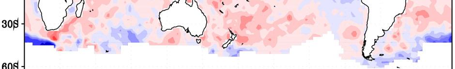
28 2.5 Sea surface temperatures in the western North Pacific Positive SST anomalies exceeding +1ºC prevailed from the Bering Sea to the seas far off east of Japan from June to September 23. Negative anomalies persisted east of Honshu throughout the year. In August, negative anomalies prevailed around Japan north of 35 N, and those exceeding -2ºC were found southeast of Hokkaido (Figure 2.7(a)). Negative SST anomalies east of Honshu and positive anomalies far off east of Japan are clearly found in the annual mean SST anomaly (Figure 2.7(b)). The value of annual mean anomaly east of Honshu exceeded -1ºC. Positive anomalies exceeding +.5ºC were found south of Honshu and in the equatorial Pacific near the date line, where anomalies remained positive almost throughout the year. (a) (b) Figure 2.7 Sea surface temperature (SST) anomalies (ºC) in the western North Pacific. (a) Monthly mean anomalies in August 23 and (b) annual mean anomalies against normal ( average) in

29 2.6 Sea Ice in the Sea of Okhotsk From December 22 through May 23, sea ice extent in the Sea of Okhotsk was below normal (normal: 3-year average from 197/1971 to 1999/2) in the period from early to middle December and from middle to late May and above normal in the period of middle January, late February and from late March to middle April (Figure 2.8). Sea ice extent recorded its maximum of km 2, which is larger than the normal annual maximum ( km 2 ), on 28 February. This indicates that about 8% of the sea of Okhotsk was covered with sea ice. Accumulated sea ice extent, which is the sum of every 5-day sea ice extent from December to May and used as an index of the magnitude of sea ice extent in the current sea ice season, has been above normal for the recent six consecutive years (Figure 2.9). Figure 2.8 Seasonal variations of sea ice extent from December 22 to May 23 in the Sea of Okhotsk. The normal is 3-year average from 197/1971 to 1999/2. Figure 2.9 Interannual variations of sea ice extent (blue bar) and its annual accumulation (red bar) in the Sea of Okhotsk. 26

30 2.7 Sea level trend around Japan The time series of annual mean sea level observed from 197 to 23 at 13 stations (Figure2.1) are shown in Figure2.11. It indicates that the sea level around Japan has risen since the middle of 198 s. The highest values over the period were recorded during the last 5 years except Hakodate. In 23, compared with 22 when the area-averaged annual mean sea level was the highest in the past 1 years, sea levels rose up on the south coast of Japan but fell down on the north coast of Japan and Sea of Japan. Especially at Kushimoto and Mera the sea levels in 23 were highest during the last three decades. Table2.5 shows the rates of the sea level rise from 197 to 23. It is recognized that the sea levels have risen at most stations. The maximum rate of 9.3 mm/year is observed at Kushiro. These rates contain the effect that the sea level appears to rise or fall by the crustal movement. To estimate the sea level trend over recent decades around Japan, Figure2.1 Location of 13stations around Japan for monitoring the sea level rise. 27

31 { Wakkanai Abashiri The annual mean sea levels 1cm Kushiro Hakodate Ofunato Mera Chichijima Kushimoto Aburatsu Naha Nagasaki Hamada Toyama Year Figure2.11 The time series of the annual mean sea levels at 13 stations around Japan. Each horizontal line shows the mean value of each station from 197 to 23 (from 1976 to 23 at Chichijima). A vertical scale is equivalent to 1 cm. Table2.5 The rates of sea level rise (mm/year) at the stations around Japan from 197 to 23 (from 1976 to 23 at Chichijima). Wakkanai Abashiri Kushiro Hakodate Ofunato Mera Chichijima Kushimoto Aburatsu Naha Nagasaki Hamada Toyama

32 3 Monitoring of greenhouse gases and ozone depleting substances JMA has been continuously measuring the concentrations of greenhouse gases such as carbon dioxide (CO 2 ) and methane (CH 4 ) at three stations (Figure 3.1): Ryori, Minamitorishima, and Yonagunijima. JMA has also carried out an observation of greenhouse gases at altitudes of 8-13 km by commercial flights between Japan and Australia. Furthermore, concentrations of greenhouse gases over the ocean and in seawater are regularly monitored by JMA research vessels in the western North Pacific. Atmospheric turbidity observations are conducted at 14 stations in Japan for studying influences of aerosol on the global climate. Such observations have been made systematically as a part of international frameworks such as the Global Atmosphere Watch (GAW) programme of the World Meteorological Organization (WMO). JMA also operates the WMO World Data Centre for Greenhouse Gases (WDCGG) to collect, archive, and distribute the data of greenhouse gases in the world. The archived data can be accessed from all over the world through the Internet ( so that the data contributes to various studies for the carbon cycle among the atmosphere, ocean, and biosphere, and for projections of the global warming. Figure 3.1 Locations map of observation stations for greenhouse gases (3 stations), direct solar radiation (14 stations), and ozone layer and UV-B radiation (5 stations). 29

33 3.1 Greenhouse Gases and Ozone Depleting Substances in the Atmosphere Table 3-1 shows the global concentrations of greenhouse gases in 22 that were reported to the WDCGG by 23. The global mean atmospheric CO 2 concentration has been steadily increasing. The global mean of the atmospheric CH 4 and N 2 O concentrations did not show distinctive growths. The global mean of CO concentration, which is not a greenhouse gas but affects the concentrations of greenhouse gases, slightly increased. Table 3.1 The global mean concentrations of greenhouse gases in 22. Atmospheric concentration Parameter Pre-industrial Global mean in 22 Increase level (Growth rate from pre-industrial from 21 level) CO 2 ~ 28 ppm ppm (+33%) CH 4 ~ 7 ppb 1782 ppb ppb (+155%) N 2 O ~ 27 ppb 317 ppb.5 ppb (+17%) lifetime (year) Property Radiative forcing** (W/m 2 ) 1.8 ppm 5~ CO* 98 ppb 5 ppb ~.25 - * CO is not a greenhouse gas, but it affects atmospheric concentrations of greenhouse gases through various chemical reactions. ** Radiative forcing is a measure of the influence a factor has in altering the balance of incoming and outgoing energy in the Earth-atmosphere system, and is an index of the importance of the factor as a potential climate change mechanism. It is expressed in Watts per square meter (Wm -2 ) Carbon Dioxide CO 2 contributes most significantly, of all greenhouse gases, to the global warming. The atmospheric concentration of CO 2 has been increasing with emissions from various human activities such as combustion of fossil fuels, production of cement, and deforestation. Among them, the combustion of fossil fuels accounts for about three fourths of all the anthropogenic CO 2 emission (IPCC, 21). Figure 3.2 shows time series of the atmospheric CO 2 concentrations at three stations in the world: Ryori (Japan), Mauna Loa (Hawaii, USA), and the South Pole. Atmospheric CO 2 has been observed since 1957 at the South Pole, since 1958 at Mauna Loa, and since 1987 at Ryori. The atmospheric CO 2 concentration at the South Pole or Mauna Loa was about 315 ppm at the beginning and has been increasing gradually with seasonal variation. The analysis by the WDCGG shows that the globally averaged atmospheric CO 2 concentration was ppm in 22, and it was 33% higher than the concentration in the 18th century (about 28 ppm) (JMA/WMO, 23). 3

34 Figure 3.2 Time series of monthly-mean atmospheric CO 2 concentrations at Ryori (Japan), Mauna Loa (Hawaii, USA), and the South Pole from 1958 to 23 based on the data from WDCGG and the Carbon Dioxide Information Analysis Center in USA. Figure 3.3 Three-dimensional representations of the annual variations of atmospheric CO 2 latitudinal distribution (concentrations (a) and growth rates (b)) for the period The analysis is based on the data archived by the WDCGG. Figure 3.3 shows the annual variations of zonally-averaged atmospheric CO 2 concentrations and growth rates from 1983 to 22 that are produced by the WDCGG using the archived data from all over the world. The seasonal variation with decreasing from spring to summer and increasing from summer to the following spring is mainly due to the activity of the terrestrial biosphere. The seasonal variation is smaller in the Southern Hemisphere because the land area is small. From the deseasonalized 31

35 variation, the CO 2 concentrations are high in mid- and high latitudes in the Northern Hemisphere while they are decreasing toward southern latitudes. This latitudinal distribution of CO 2 concentration is ascribed to the existence of many CO 2 sources in mid- and high latitudes in the Northern Hemisphere. In both hemispheres, the atmospheric CO 2 concentrations are increasing year by year. The global mean growth rate during was 1.6 ppm/year. Figure 3.4 shows monthly-mean atmospheric CO 2 concentrations, deseasonalized concentrations, and growth rates at Ryori, Minamitorishima, and Yonagunijima. The deseasonalized concentration is obtained by filtering out variations with shorter time scales than the seasonal variation. At all stations, the CO 2 concentrations increase, accompanying with the seasonal variation that is caused by photosynthesis and respiration of the biosphere. The CO 2 concentration at Yonagunijima is, in general, higher than that at Minamitorishima while they are located almost the same latitude. This reflects influences of anthropogenic emissions throughout a year and biospheric emissions from autumn to the following spring from the Asian continent that is closely located upwind of Yonagunijima. The annual mean CO 2 concentrations in 23 were ppm at Ryori, ppm at Minamitorishima, and ppm at Yonagunijima. Compared with the concentrations in the previous year, CO 2 increased by 2.7 ppm at Ryori and 2.8 ppm at Minamitorishima and Yonagunijima. Figure 3.4 Time series of monthly-mean atmospheric CO 2 concentrations, deseasonalized concentrations (a), and growth rates (b) at Ryori, Minamitorishima, and Yonagunijima. Figure 3.5 shows time series of the atmospheric CO 2 concentrations over the Pacific at altitudes of 8-13km by an aircraft observation using commercial flights between Japan and Australia in cooperation with the Japan Air Line Foundation, the Ministry of Land, Infrastructure and Transport, and the Japan Airlines. The CO 2 concentrations increase with seasonal variations like those on the surface. The seasonal variations observed over the Northern Hemisphere also reflect those on the surface, but the amplitudes are smaller. In the Southern Hemisphere, the variations are complicated with double peak seasonality. 32

36 Figure 3.5 Time series of CO 2 concentrations (dots), fitting curves (black solid line), deseasonalized concentrations (blue dashed line), and growth rates (red solid line) averaged in each 5-degree latitudinal zone observed at altitudes of 8-13 km. The data used in this analysis were collected by commercial flights between Japan and Australia. The global growth rates of CO 2 concentrations are not constant. Figure 3.3 shows globally higher growth rates during 1983, , , and On the other hand, a negative growth rate was observed in northern high latitudes during The corresponding variations of CO 2 growth rates were observed at three Japanese stations as shown in Figure 3.4 and at high altitudes over the Pacific Ocean as shown in Figure 3.5. A rapid increase of CO 2 growth rate from 1997 to 1998 and the following decrease are related with the El Niño event during El Niño events have two opposite effects on the atmospheric CO 2 concentration. During an El Niño event, suppression of CO 2 -rich ocean-water upwelling reduces CO 2 emissions from the ocean into the atmosphere in the eastern tropical Pacific. On the other hand, warmer and drier weather caused by an El Niño event strengthens CO 2 emissions from the terrestrial biosphere, particularly in the tropical regions, which are caused by plant respiration, decomposition of organic soil, and depression of photosynthesis. The latter effect dominates over the former, which brings about a net CO 2 increase in the atmosphere with several month delay (Keeling et al., 1989; Nakazawa et al., 1993; 33

37 Dettinger and Ghil, 1998). The scarce precipitation that brought about the droughts and the frequent forest fires in Southeast Asia in 1997/1998 and the remarkable high global mean temperature in 1998 are considered to have strengthened CO 2 emissions from the terrestrial biosphere (Watanabe et al., 2). Although the El Niño event occurred during , the growth rate decreased significantly during this event. The increase in absorption of CO 2 into the terrestrial biosphere and the ocean, which was resulted from global cooling by the eruption of Mt. Pinatubo, brought about the growth rate decrease (Rayner et al., 1999). These inter-annual variations in CO 2 growth rate can be interpreted as fluctuations of the carbon cycle that is influenced by climate. Since these fluctuations in the carbon cycle can affect climate through the global warming, it is necessary to clarify the carbon cycle system including the inter-annual variations to achieve an accurate projection of the global warming Methane CH 4 is a second most significant greenhouse gas after CO 2, and emitted into the atmosphere from various sources including wetlands, rice paddy field, ruminant animals, natural gas production, and biomass burning. CH 4 is primarily removed from the atmosphere by photochemical reaction with hydroxyl (OH) radicals. The analysis by the WDCGG shows that the globally averaged atmospheric CH 4 concentration was 1782 ppb in 21 (JMA/WMO, 23). The concentration is almost 2.5 times as large as the concentration before the 18th century (about 7 ppb). The annual mean CH 4 concentrations at JMA stations in 22 were 18 ppb at Minamitorishima, 1854 ppb at Ryori, and 1819 ppb at Yonagunijima. Figure 3.6 shows time series of atmospheric CH 4 concentrations observed at Minamitorishima, Mauna Loa, and the South Pole. The CH 4 concentrations have a seasonal variation: decreasing from winter to summer and increasing from summer to winter. This is mainly due to the seasonality of OH radicals that destroy CH 4, because OH concentration rises in summer by abundant water vapor and intense ultraviolet radiation. Figure 3.6 Time series of monthly-mean atmospheric CH 4 concentrations at Minamitorishima (Japan), Mauna Loa (Hawaii, USA), and the South Pole based on the archived data by the WDCGG. 34

38 Figure 3.7 shows variations of zonally-averaged atmospheric CH 4 concentrations from 1984 to 22 that are produced by the WDCGG using archived data from all over the world. The concentrations have been increasing from year to year with seasonal variation in all latitudes. The concentrations decline from mid- and high latitudes in the Northern Hemisphere toward south. This is due to the fact that sources of CH 4 are mainly on the land and that the Northern Hemisphere has larger land areas than the Southern Hemisphere. Generally, growth rates in the 199s are lower than those in the 198s. In 198s, global CH 4 concentrations increased with growing emissions from anthropogenic sources such as agriculture and industry. They may be, however, approaching the steady state where removal of CH 4 is balanced with emissions from the sources (Etherridge et al., 1998; Dlugokencky et al., 23). It is necessary to watch continuously this situation. Figure 3.7 Three-dimensional representations of the annual variations of atmospheric CH 4 latitudinal distribution (concentrations (a) and growth rates (b)) for the period The analysis is based on the data archived by the WDCGG. In this nearly steady situation, even minor variations of emission or removal can influence the variations of growth rates. In the 199s, the global CH 4 growth-rates variation was accompanied with the global mean temperature anomaly. The growth rates rose in 199, 1991, 1994, 1995, 1997, and 1998 when the global mean temperature anomalies from the average exceeded +.4 C. On the other hand, the grow rates fell down in 1992, 1993, and 1996 when the global mean temperature anomalies were between +.1 C and +.2 C. High temperature anomaly brings about, on one hand, an increased CH 4 emission from wetlands and, on the other hand, an increased uptake by increased OH radicals (Bekki and Law, 1997). The large growth rates during the high positive temperature anomaly show that the former effect globally dominates over the latter. This effect emerged clearly in the 199s when the long-term growth was getting slow. Considering that CH 4 is one of the major greenhouse 35

39 gases, the relationship between variations of CH 4 concentration and global temperature indicates an importance of the emission and removal process of CH 4 for an improvement of the global warming projection Nitrous Oxide Nitrous oxide (N 2 O) is a greenhouse gas with a long lifetime (the quantity that the total amount in the atmosphere is divided by the decomposition rate per year) of about 114 years in the atmosphere. N 2 O is emitted into the atmosphere from soil, the ocean, use of nitrate and ammonium fertilizers, and various industrial processes. N 2 O is photodissociated in the stratosphere by ultraviolet radiation. The concentration of atmospheric N 2 O has been increasing globally. The global mean concentration of atmospheric N 2 O was 317 ppb in 22. This concentration was about 17% higher than the concentration before the 18th century (about 27 ppb) (IPCC, 21). Figure 3.8 shows time series of monthly-mean N 2 O concentration in the atmosphere observed at Ryori. Short-term variation is very weak and no seasonal variability is observed. The annual mean N 2 O concentration was 319 ppb in 23, showing still slightly increasing trend. Figure 3.8 Time series of monthly-mean atmospheric N 2 O concentrations at Ryori. Error bars in the figure represent the standard deviations estimated from daily mean concentrations Halocarbons Halocarbons are carbonic compounds with fluorine, chlorine, bromine, or iodine. Most of them do not exist in the natural atmosphere but are chemically manufactured. They do not only destroy stratospheric ozone, but also warm the global atmosphere directly as greenhouse gases and, at the same time, cool the lower stratosphere indirectly through ozone destruction in the stratosphere. The atmospheric concentrations of most halocarbons are less than a millionth of that of CO 2. However, they contribute significantly to the global warming because their radiative effects per unit mass are several thousand times larger than that of CO 2. Furthermore, the effects can last very long because of their long lifetimes in the atmosphere. Chlorofluorocarbons (CFCs), which are compounds of carbon, fluorine, and chlorine, are important substances in halocarbons. Emissions of CFCs have been regulated by the Montreal Protocol on Substances that Deplete the Ozone Layer. Consequently, the observation by the Atmospheric Lifetime Experiment/Global Atmospheric Gases Experiment (ALE/GAGE) shows that the CFC-11 concentration was at the peak in 1993 and has declined since The CFC-12 concentration has been 36

40 increasing while the growth rate has become much lower, and the CFC-113 concentration has stopped increasing since 1996 (WMO, 1999). Figure 3.9 shows time series of monthly mean concentrations of CFC-11, CFC-12, and CFC-113 in the atmosphere observed at Ryori, indicating weak short-term variations and no seasonal variability. The CFC-11 concentration had a peak of about 28 ppt during and a decreasing trend since then. The CFC-12 concentration has almost stopped increasing for the last few years. The CFC-113 concentration indicates little change. The annual mean concentrations in 23 were about 26 ppt for CFC-11, about 54 ppt for CFC-12, and about 8 ppt for CFC-113. Hydrochlorofluorocarbons (HCFCs), hydrofluorocarbons (HFCs), and perfluorocarbons (PFCs), which are used as substitutes for CFCs, have been increasing in the atmosphere. For example, the observation by the Climate Monitoring and Diagnostics Laboratory (CMDL) in the National Oceanic and Atmospheric Administration (NOAA) showed that the total chlorine concentration from major three HCFCs was 19 ppt and the increasing rate was about 8-9 ppt/year (CMDL, 22). They also showed that the concentration of HFC-134a was 17.2 ppt in 21, and the increasing rate was 3.2 ppt/year during CMDL also reported that the concentration of SF 6, which is an effective gaseous dielectric and enclosed in electrical equipment, was almost 5 ppt in the middle of 21 and had been increasing linearly by.22 pptv/year since HFCs, PFCs, and SF 6 are the greenhouse gases, as well as CO 2, CH 4, and N 2 O, which are subject to the Kyoto Protocol to the United Nations Framework Convention on Climate Change. Figure 3.9 Time series of monthly-mean concentrations of atmospheric CFC-12 (top), CFC-11 (middle), and CFC-113 (bottom) at Ryori. Error bars represent the standard deviations calculated from daily mean concentrations Carbon Monoxide Sources of carbon monoxide (CO) are emissions from industrial and agricultural combustion and production from oxidation of hydrocarbons including methane. It is mainly removed through a reaction with OH radicals in the atmosphere. CO is not a greenhouse gas in itself because it hardly absorbs 37

41 infrared radiation from the earth s surface. However, CO is controlling many greenhouse gases through production of OH radicals as well as a precursor of tropospheric ozone (Daniel and Solomon, 1998). Figure 3.1 shows time series of monthly-mean atmospheric CO concentrations and deseasonalized concentrations at Ryori, Minamitorishima, and Yonagunijima. The concentrations show seasonal variations with a peak from winter to early spring and a depression in summer. An increase in the CO concentration was seen from 1997 to 1998, suggesting influences of the forest fires in Indonesia and Siberia. The annual mean concentrations in 23 were 175 ppb at Ryori, 132 ppb at Minamitorishima, and 162 ppb at Yonagunijima. The lifetime of CO in the atmosphere is 2~3 months, resulting in large spatial and temporal variations that depend on the local emissions. The east coast of the Asian continent is considered as one of the active CO emission areas due to less efficient combustion from burning of biofuel (Wang et al., 21). The concentration at Yonagunijima is higher than that at Minamitorishima while both stations locate almost in the same latitudinal zone. This is due to that Yonagunijima is frequently influenced by the CO emissions in the Asian continent. Figure 3.1 Time series of monthly-mean atmospheric CO concentrations and deseasonalized concentrations at Ryori, Minamitorishima, and Yonagunijima. The analysis by the WDCGG shows that the globally averaged atmospheric CO concentration was about 98 ppb in 22 (JMA/WMO, 23). The analysis of ice cores shows that the concentration of CO in Antarctica, approximately 5 ppb, indicates little change for the last 2 years (Haan and Raynaud, 1998). They also suggested that the concentration of CO in Greenland had been about 9 ppb before the middle of 19th century, and had gradually increased to about 11 ppb in 195. Figure 3.11 shows the annual variations of latitudinal distribution of CO concentration and growth rate for the period The seasonal cycle with high concentrations from winter to spring and low concentrations in summer is obvious. The concentrations are high in northern mid-latitudes and low in Southern Hemisphere, indicating that the major sources are in the northern mid-latitudes and the concentration decreases with transporting to the equatorial area that is a major sink region of CO (JMA, 23). The concentrations from the equatorial area to the northern mid-latitudes had enhanced from 1997 to The large-scale biomass burning in Indonesia in 1997 and forest fires in Siberia from summer to autumn in 1998 influenced the enhancement of CO (Novelli et al., 23). 38

42 Figure 3.11 Three-dimensional representations of the annual variations of atmospheric CO latitudinal distribution (concentrations (a), and growth rates (b)) for the period This analysis is based on the data archived by the WDCGG Tropospheric Ozone Tropospheric ozone (O 3 ) is one of the important greenhouse gasses. Tropospheric ozone is also a chemically reactive gas and produces OH radicals that control atmospheric concentrations of many greenhouse gases through chemical reactions. Tropospheric ozone is produced from photochemical oxidation of CH 4, CO, and non-methane hydrocarbons (NMHCs) under the nitrogen oxides (NO x ) rich environment. O 3 is removed by reactions with hydrogen oxides (HO x, i.e., HO 2 and OH). In mid- and high latitudes, ozone is transported from the stratosphere down to the troposphere, and also destroyed on the earth s surface. The concentration varies significantly with locations, altitudes, and seasons. Figure 3.12 shows time series of monthly-mean surface ozone concentrations and deseasonalized concentrations at Ryori, Minamitorishima, and Yonagunijima. The concentration at Ryori has slightly increased since the beginning of observation in 199. The concentrations usually show seasonal variations with a peak from spring through early summer and a depression in midsummer. While Yonagunijima is located in the same latitudes as Minamitorishima, the concentration at Yonagunijima is usually higher than that at Minamitorishima. In the eastern region of China, the peak of the monthly mean concentrations is observed in autumn; the maximum at the Changjiang River Delta is higher than 6 ppb (Chameides et al., 1999). The concentrations at Yonagunijima are higher than those at Ryori from autumn to early spring. The ozone-rich air masses are supposed to be transported from the Asian continent to Yonagunijima. The annual mean concentrations in 23 were 41 ppb at Ryori, 28 ppb at Minamitorishima, and 43 ppb at Yonagunijima. 39

43 Figure 3.12 Time series of monthly-mean surface ozone concentrations and deseasonalized concentrations at Ryori, Minamitorishima, and Yonagunijima. 3.2 Oceanic Carbon Dioxide It is very important to evaluate how much the anthropogenically released CO 2 is taken up by the ocean in order to project future concentration of atmospheric CO 2 and its resultant global warming. On a global scale, it is estimated that the ocean absorbs CO 2 at about 2 PgC ( g carbon) per year (IPCC, 21). On a regional scale, however, the amount of the oceanic CO 2 uptake differs from place to place. Besides, some regions such as the equatorial Pacific emit CO 2 and other regions change its role as a sink or source for atmospheric CO 2 depending on seasons. These geographical inhomogeneity and seasonal variations of the behavior of the ocean make it difficult to estimate oceanic CO 2 uptake. It is necessary to evaluate the absorption or emission amount of CO 2 quantitatively for each region and season in order to reduce the uncertainty of the estimate. JMA has conducted ship observations for greenhouse gases (CO 2, CH 4, CFCs and N 2 O) in the sea surface air and in the surface seawater in the western North Pacific using the research vessels Ryofu Maru and Keifu Maru. JMA has periodically made the CO 2 observations along 137 E in winter since Figure 3.13 shows the long-term variation of atmospheric and oceanic CO 2 concentrations in January and February averaged between 3 N and 3 N along 137 E. In this region, the concentration of oceanic CO 2 is lower than that of atmospheric CO 2, suggesting that the ocean acts as a sink for atmospheric CO 2 in winter. The concentrations of both the atmospheric and oceanic CO 2 in this region have increased at the mean growth rate of about 1.6 ppm/year from 1981 to 23. The oceanic CO 2 has larger inter-annual variability compared with the relatively monotonic increase in the atmospheric CO 2. Although the rapid mixing of air forms uniform atmospheric CO 2 concentration, surface oceanic CO 2 concentration varies largely year by year, because the magnitude of entrainment of CO 2 -rich water from the lower layer to the surface layer depends on the strength of surface wind stress and surface heating/cooling. 4

44 Figure 3.13 Time series of the concentrations of atmospheric and oceanic CO 2 along 137 E (the average of 3 N-3 N) in winter (January-February) from 1981 to 23. In the subtropical western North Pacific, the concentration of oceanic CO 2 has closely correlated with the sea surface temperature (Inoue et al., 1995). Using the empirical interpolation method based on this high correlation, the concentration of oceanic CO 2 and the air-sea partial pressure difference of CO 2 can be estimated in the seasons and the regions of no observed CO 2 data (Murata et al., 1996). Furthermore, with the calculated air-sea partial pressure difference of CO 2 and the monthly mean wind speed distribution over the ocean, air-sea CO 2 exchange flux can be estimated. JMA has conducted the ship observation along 165 E by the research vessel Ryofu Maru since Accordingly, an estimate of the time series of CO 2 flux in the western North Pacific has become possible using the observation results along 165 E in addition to those along 137 E. Figure 3.14 shows the time series of the annual net CO 2 flux from 1996 to 22 in the western North Pacific (11 N-3 N and 13 E-165 E). The ocean in this region acts as a source in summer and a sink in winter for the atmospheric CO 2. This region, however, acts as a net sink on a yearly base, because the absorption amount of CO 2 in winter is estimated to be greater than the emission amount in summer. The estimated annual net flux in this region has fluctuated between 3 TgC ( g carbon) and 85 TgC per year during the period. 41

45 Figure 3.14 The annual variation of net CO 2 flux in the subtropical region in the western North Pacific (11 N-3 N and 13 E-165 E) from 1996 to 22. The unit is teragram (1 12 gram) of carbon per year and positive values mean the uptake by the ocean. The gas transfer formulation is based on Tans et al. (199), and the gas transfer coefficient is calculated using surface-wind speed data from monthly-mean objective-analysis data provided by JMA. The oceanic CO 2 concentration in the equatorial Pacific (156 E-165 E) in autumn has been usually higher than the atmospheric CO 2. However, the difference between the concentrations of atmospheric and oceanic CO 2 was small in October 1997 and October 22 when the El Niño event occurred (Figure 3.15). This is due to the reduction of upwelling of CO 2 -rich water from a lower layer, covered with the thick warm water during the El Niño events. In July 23, the difference between the concentrations of atmospheric and oceanic CO 2 was also smaller than that in a normal year, suggesting that the emission amount of CO 2 was small in this region. This is supposed to be attributed to the ocean condition that was still covered with the warm water just after the El Niño event had terminated. Figure 3.15 Time series of the concentrations of atmospheric and oceanic CO 2 in the equatorial Pacific (the average of 156 E-165 E) from 1996 to 23. Observations were performed in October to November and in July 23. Red areas represent periods of El Niño event and blue areas represent periods of La Niña event. 42

46 3.3 Aerosols Small particles floating in the atmosphere are called aerosols. Aerosols directly and indirectly affect climate. Directly, aerosols decrease the global temperature because it scatters and absorbs solar radiation. On the other hand, it also warms the atmosphere by absorbing and reemitting infrared radiation from the earth s surface. Indirectly, the aerosol changes the characteristics of cloud by acting as cloud condensation nuclei (CCN), resulting in the change of the planetary albedo. While the large uncertainties still remain in contribution of these opposite effects to climate change, an increase in the aerosol amount is estimated to decrease the surface temperature on a global scale Turbidity coefficient by Direct solar-radiation measurement JMA has been monitoring direct solar-radiation at 14 stations in Japan to obtain the Feussner-Dubois turbidity coefficient that is information on atmospheric turbidity. The turbidity coefficient is an index of impurity of the atmosphere caused by the turbid constituents such as aerosol, water vapor, ozone, and CO 2. The turbidity coefficient is expressed as the ratio of solar radiation extinction in the observed atmosphere to that in the ideal atmosphere that includes no such impurity. A larger value means that more turbid constituents are loaded in the atmosphere. Figure 3.16 shows time series of Feussner-Dubois turbidity coefficient at Nemuro, Matsumoto, Shionomisaki and Ishigakijima (see Figure 3.1) in 23. At the first three stations, the turbidity coefficients in summer were larger than those in winter mainly due to the seasonality of water vapor. Ishigakijima is an island that had little seasonal variation of water vapor, and the turbidity coefficient in spring was larger mostly due to the influence of the aeolian dust, which is called yellow sand and frequently comes from the Asian continent in spring. 43

47 Figure 3.16 Time series of the Feussner-Dubois turbidity coefficients at Nemuro, Matsumoto, Shionomisaki and Ishigakijima in 23. The daily minimum are selected in which the hourly mean meets following three condition: sun is shining, solar elevation is high (optical air mass 2.5), and the difference between maximum and minimum of direct solar radiation within 5 minutes is less than.3 kw/m 2. A solid line in the figure indicates smoothed monthly mean values at local noon for Figure 3.17 shows a yearly variation of the Feussner-Dubois turbidity coefficient from 1961 to 23 in which the shorter variations than seasonal variation are filtered out. In this analysis, the monthly minimum values averaged over 14 stations in Japan are used to avoid influences of water vapor and severe dust events that varies largely day by day. The enhancements of Feussner-Dubois turbidity coefficient in the periods of and are due to the eruptions of Mt. El Chichon (Mexico) in 1982 and Mt. Pinatubo (Philippines) in 1991, respectively. Both eruptions put a huge volume of volcanic ash and SO 2, which is a precursor of sulfate aerosol, into the stratosphere. At present, the Feussner-Dubois turbidity coefficient has returned to the level before the eruption of Mt. El Chichon. 44

48 Figure 3.17 Smoothed time series of the Feussner-Dubois turbidity coefficient from 1961 to 23 averaged over 14 stations in Japan. The monthly minimum values are used in order to minimize influences of water vapor and severe dust events, and the variations with shorter time scales than seasonal variation are filtered out Aerosol Optical Depth observed with Sunphotometer JMA has been carrying out aerosol optical depth (AOD: an index of the atmospheric turbidity by aerosols) observation with Sunphotometer three times a day, 9, 12, 15 JST (Japan Standard Time) at Ryori, 8, 11, 14 JST at Minamitorishima, 1, 13, 16 JST at Yonagunijima. The data are not obtained when clouds cover the sun at the time of observation. The Sunphotometers are calibrated by using the Langley method. The Langley plot is performed at Komagane (2612 m a.s.l.) in Nagano prefecture in autumn every year, in accordance with the WMO guidance (WMO, 1993). Figure 3.18 shows the time series of aerosol optical depth and Ångström exponent (α: an index of aerosol size distribution, the larger value indicates smaller size distribution of aerosols) observed at Ryori, Minamitorishima and Yonagunijima in 23. While the AOD at Minamitorishima kept lower values through the year, the variations of AOD were relatively large at Ryori and Yonagunijima. These variations of the two stations might be ascribed to the influence of aeolian dust (yellow sand) from the Asian continent, biomass burning, and anthropogenic pollutants. 45

49 Figure 3.18 Time series of Aerosol Optical Depth (AOD) and Ångström exponent (α) observed at Ryori, Minamitorishima and Yonagunijima in 23. JMA presumed that a peak of AOD at Ryori in May 23 originated from the smoke of the forest fires in Siberia. The Ångström exponents in Minamitorishima were relatively small, indicating that the dominant aerosol particles were relatively large The vertical profiles of aerosols observed by lidar system JMA has routinely observed vertical profiles of aerosol using a lidar system at Ryori since March 22. Lidar is also called as a laser radar, and it shoots a laser pulse upward and receives the light scattered by aerosols or air molecules with telescopes. Figure 3.19 shows 3-month mean aerosol vertical profiles (scattering ratio) in 23. The vertical profiles of scattering ratio show that the aerosol amount of the stratosphere was quite less than that in the troposphere, and the aerosol amount in the troposphere had a large variety in season. There are more aerosols in the lower troposphere because the sources of aerosols mainly exist at the earth s surface. In spring time, the mean aerosol amount in the middle troposphere was larger than the other seasons. The aeolian dust (yellow sand) that is transported from the Asian continent in spring is supposed to cause this increment. 46

50 Figure 3.19 Vertical profiles of 3-month averaged (only clear days) scattering ratio observed by the lidar system at a wavelength of 532nm (solid line), and its standard deviations (shaded area) at Ryori in 23. Climate is influenced by not only aerosols in the stratosphere originating in sporadic and extensive volcanic eruptions but also aerosols in the troposphere such as mineral dust, sulfate aerosol, and soot particles emitted from fossil fuel combustion. However, their global and regional distributions and temporal variations have not been clearly understood yet. It is necessary to clarify the characteristics of aerosols for improvement of the global warming projection. Lidar system is expected as one of the effective means to clarify the characteristics of aerosols.. 47

51 4 Monitoring of the ozone layer and ultraviolet B (UV-B) radiation Depletion of the ozone layer has been observed over Antarctica mainly from September through November since the early 198s. This phenomenon is called "ozone hole". The ozone hole, which appears over Antarctica under its unique meteorological conditions resulting from the Antarctic topography and polar night, is mainly caused by man-made chlorofluorocarbons (CFCs) and halons. CFCs and halons have been widely used for various purposes such as cleaning solvents, aerosol propellants, refrigerants, and fire extinguishers, by their excellent characteristics such as chemical stability. Due to their stability, however, CFCs are hardly decomposed in the troposphere and spread gradually into the stratosphere, where CFCs are decomposed into chlorine atoms that destroy ozone molecules. Ozone layer depletion, which is typically characterized by the ozone hole, is observed in both hemispheres except equatorial zone. Ozone layer is depleted as in the following process. When CFCs reach the altitude of about 4 km in the stratosphere, solar ultraviolet radiation detaches free atomic chlorines from CFCs. The atomic chlorine, while moving in the stratosphere, reacts with and destroys ozone around them, changing it to chlorine monoxide, which turn back to atomic chlorine again reacting with atomic oxygen and other molecules. The released atomic chlorine reacts with and destroys ozone again. These processes occur in a virtual chain reaction and destroy ozone repeatedly. 4.1 Observational results of the ozone layer in Global ozone layer As for the total ozone in 23, negative anomalies (against monthly mean value of satellite data from 1979 to 1992) generally prevailed. Based on the total ozone data by satellites, the global decreasing trends are obvious except in the tropics. The decreasing trends are larger in higher latitudes in springtime Ozone layer over Japan JMA has been carrying out ozone layer observations at Sapporo, Tsukuba/Tateno, Kagoshima, and Naha since 1957, and at Minamitorishima since 1994 (see Figure 3.1). Hereafter, 'almost normal' indicates values within the standard deviation from the monthly mean values and 'higher/lower than normal' values are higher/lower than 'almost normal' in this section. As shown in Figure 4.1, the monthly means of total ozone over Japan in 23 were generally higher at Naha, and lower in the end of the year at Sapporo, Tsukuba and Kagoshima. The monthly means of total ozone were 'lower than normal' in April, November, and December at Sapporo, November at Tsukuba, November and December at Kagoshima. The monthly means of total ozone were 'higher than normal' in July, and August at Sapporo, January, March, June and July at Tsukuba, January at Kagoshima, January, March and from June to October at Naha. The highest values in March, July and 48

52 October at Naha were recorded as the months since the beginning of monitoring. The monthly means of total ozone in the former half of 23 were higher than the normal at Minamitorishima. Figure 4.1 Monthly means of total ozone at five stations in Japan: Sapporo, Tsukuba/Tateno, Kagoshima, Naha, Minamitorishima, and Syowa Station (Antarctica). Closed circle indicates observations in 23 and solid lines indicate monthly mean values with bars of standard deviation ( but in Naha and in Minamitorishima). As for Syowa, a solid line indicates monthly mean values before the appearance of the ozone hole ( ) and a dotted line indicates those after the appearance (1981-2). The decreasing trends in total ozone are seen at all of the stations except Naha (Figure 4.2). In particular, this trend is most remarkable at Sapporo. Based on the vertical distributions of ozone concentration, the decreasing trends in the lower stratosphere over Sapporo are significant. Figure 4.2 Annual mean total ozone at four stations in Japan. The solid lines indicate long-term trends Ozone layer over Antarctica In 23, after the total ozone became lower than or equal to 22 m atm-cm (an index of ozone hole) in mid-august, almost the minimum levels of total ozone were recorded over the Syowa station from September to October. The monthly mean in September at Syowa Station was lowest since the 49

53 beginning of monitoring. The total ozone largely varied in November, and then rose to around 3 m atm-cm after the end of the November. Based on ozonesonde data on September 26, 23 when the Syowa station was located inside the ozone hole, the ozone decreased to almost zero at the altitudes of 15-2 km over the Syowa station (Figure 4.3). Figure 4.3 Vertical profiles of ozone partial pressure over the Syowa station on September 26, 23 (red solid line), and monthly mean in September during (dashed line). The satellite data showed that the area of ozone hole expanded rapidly in the end of August over the Antarctic region, and covered whole Antarctica in the early September. The annual maximum area of the ozone hole was recorded in the end of September. After that, the ozone hole reduced rapidly, and disappeared in December 8, 23 (Figures 4.4 and 4.5). Figure 4.4 Total ozone distribution in the Southern Hemisphere on September 24, 23 from TOMS data supplied by NASA. 5

54 Figure 4.5 Area of ozone hole (defined as extent of total ozone 22 m atm-cm). Left figure shows daily course of are where a red line shows values in 23 and a black line shows maximum values during Right figure shows annual course of maximum area since Ultraviolet B (UV-B) radiation in Japan As ozone strongly absorbs ultraviolet radiation, it is expected that an amount of harmful solar UV-B radiation at the earth s surface increases with decreasing the total ozone. JMA has been conducting UV-B observations at Tsukuba/Tateno since 199, and at Sapporo, Kagoshima and Naha since The monthly means of UV-B daily accumulation in 23 at 4 stations in Japan are shown in Figure 4.6. The monthly means were 'higher than normal' or 'almost normal' at all stations in Japan except in April at Sapporo, in February, May, and July at Tsukuba, and in January and June at Kagoshima, which were lower than normal. Figure 4.6 Monthly mean values of UV-B daily accumulation at four stations in Japan: Sapporo, Tsukuba/Tateno, Kagoshima, and Naha. Closed circle indicates observations in 23 and solid lines indicate monthly mean values with bars of standard deviations. 51

55 The significant trends are not seen in UV-B radiation data in Japan because the total ozone does not have significant trends over Japan after 199, which is the beginning of UV-B observation. However, the observational data under the condition of clear sky and constant solar elevation show that the UV-B radiation increases with decreasing the total ozone (Figure 4.7). Therefore, the current amount of UV-B radiation is estimated to increase compared with that in 197s. Figure 4.7 Scatter plot of UV-B radiation against total ozone. A solid line indicates a regression line. Data were obtained at four stations in Japan under clear sky conditions with a solar elevation of 23 degrees. 52