Gaia Data Release 1. Documentation release 1.1. European Space Agency and Gaia Data Processing and Analysis Consortium

Transcription

1 Gaia Data Release 1 Documentation release 1.1 European Space Agency and Gaia Data Processing and Analysis Consortium 17 February 2017

2 Executive summary We present the first Gaia data release, Gaia DR1, consisting of astrometry and photometry for over 1 billion sources brighter than magnitude 20.7 in the white-light photometric band G of Gaia. The Gaia Data Processing and Analysis Consortium (DPAC) processed the raw measurements collected with the Gaia instruments during the first 14 months of the mission, and turned these into an astrometric and photometric catalogue. Gaia DR1 consists of three parts: an astrometric data set which contains the positions, parallaxes, and mean proper motions for about 2 million of the brightest stars in common with the Hipparcos and Tycho-2 catalogues (the primary astrometric data set) and the positions for an additional 1.1 billion sources (the secondary astrometric data set). The primary set forms the realisation of the Tycho-Gaia Astrometric Solution (TGAS). The second part of Gaia DR1 is the photometric data set, which contains the mean G-band magnitudes for all sources. The third part consists of the G-band light curves and the characteristics of 3000 Cepheid and RR Lyrae stars observed at high cadence around the south ecliptic pole. The positions and proper motions in the astrometric data set are given in a reference frame that is aligned with the International Celestial Reference Frame (ICRF) to better than 0.1 mas at epoch J2015.0, and non-rotating with respect to the ICRF to within 0.03 mas yr 1. For the primary astrometric data set, the typical standard error for the positions and parallaxes is about 0.3 mas, while for the proper motions the typical standard error is about 1 mas yr 1. To the parallax uncertainties a systematic component of 0.3 mas should be added. For the subset of Hipparcos stars in the primary data set, the proper motion standard errors are much smaller, at about 0.06 mas yr 1. For the secondary astrometric data set, the typical standard error on the positions is 10 mas. The median standard errors on the mean G-band magnitudes range from the milli-magnitude level to 0.03 mag over the magnitude range 5 to The DPAC undertook an extensive validation of Gaia DR1 which confirmed that this data release represents a major advance in the mapping of the skies and the availability of basic stellar data that form the foundation of observational astrophysics. However, as a consequence of the very preliminary nature of this first Gaia data release, there are a number of important limitations to the data quality. These limitations are documented in the Astronomy & Astrophysics papers that accompany Gaia DR1, with further information provided in this documentation. The reader is strongly encouraged to read about these limitations and to carefully consider them before drawing conclusions from the data. This Gaia DR1 documentation complements the peer-reviewed papers that accompany the release in a Special Issue of Astronomy & Astrophysics. The papers form the primary documentation for the data release and they are frequently referenced throughout the text. Gaia archive; Gaia home page; Gaia A&A papers; Gaia helpdesk; Gaia FAQs; Gaia credit and citation instructions; Gaia DR1 online documentation; Gaia DR1 pdf documentation; Gaia acronym list; Gaia on Twitter and Gaia on Facebook; Gaia DR1 archive data model (column description) online documentation; Gaia DR1 archive data model (column description) pdf documentation.

3 Contents I Introduction to Gaia DR Introduction The Gaia mission Introduction and overview Mission history and science case The spacecraft The scanning law Ground segment and operations The Data Processing and Analysis Consortium Introduction History Objectives and responsibilities Structure Overview of the data processing Simulations Release framework Time coverage Scanning law Spacecraft status

4 1.3.4 Processing configuration Release properties Statistical properties Completeness Limitations II Gaia data processing 67 2 Astrometric and photometric pre-processing Introduction Overview Properties of the input data Overview The raw science telemetry data The Initial Gaia Source List (IGSL) The Gaia Ecliptic Poles Catalogue (GEPC) The Attitude Star Catalogue (ASC) Calibration models Overview Early PSF/LSF model Astrophysical background CCD cosmetics CCD bias and bias non-uniformity Processing steps Overview Daily and cyclic processing Raw data reconstruction

5 2.4.4 Basic angle variation determination On-ground attitude reconstruction (OGA1 & 2) Bias and astrophysical background determination Spectro-Photometric Image Parameters determination Astrometric Image Parameters determination Crossmatch (XM) processing Quality assessment and validation Overview Monitoring of daily pre-processing Monitoring of cyclic pre-processing Astrometry Introduction Overview Conventions, notations, nomenclature, and definitions Reference systems and time scales Standard model of stellar motion Relativistic model Time scales Transformations of astrometric data and error propagation Fundamental constants Properties of the input data Solar-system data and planetary ephemerides Ground Based Optical Tracking (GBOT) The Gaia orbit The Initial Gaia Quasar Catalogue (IGQC) BAM data

6 3.3 Calibration models Overview Aligning the Gaia reference frame Astrometric source model Attitude model Geometric instrument model Global parameters Extended PSF/LSF model Processing steps AGIS pre-processing Primary source processing (AGIS) Secondary source processing AGIS post-processing Iteration strategy and convergence AGIS-PhotPipe-IDU loop processing Quality assessment and validation Overview Properties of the astrometric data Source verification Attitude verification Geometric calibration verification Comparisons of alternative solutions Correlations in the Gaia data Comparisons with space-based astrometry Comparisons with ground-based astrometry Astronomical checks of the data

7 Conclusions The Tycho-Gaia Astrometric Solution (TGAS) Introduction Overview Properties of the input data The Hipparcos catalogues The Tycho-2 catalogues Incorporating of prior information in astrometric solutions The TGAS reference frame Processing steps The use of prior information in AGIS Epoch propagation of prior information Quality assessment and validation Photometry Introduction Overview Notations, nomenclature, and definitions Spectral Shape Coefficients Reference System Properties of the input data Overview Ground-based catalogue for external calibrations IDT/IDU data Calibration models BP/RP background model

8 5.3.2 BP/RP geometric model Flux-photometry model External calibration Photometric relationships with other photometric systems Processing steps Pre-processing BP/RP processing Standard star selection Quality assessment and validation Verification III Gaia data analysis Variability Introduction Properties of the input data Input catalogue Training sets Calibration models General time series models Time series models of Specific Objects Processing steps Initial light curves pre-processing Statistical parameter computation Variability Detection Period search and time series modelling Classification

9 6.4.6 Specific Object Studies Quality assessment and validation Verification Validation IV Gaia catalogue consolidation Catalogue consolidation and validation Introduction Overview Properties of the input data Gaia MDB data model Input data description from all DPCs Processing steps MDB Integrator Ingestion in GACS Crossmatch with external catalogues Catalogue validation Introduction Internal comparisons Confrontation to external catalogues Validation using open clusters Comparison to models Multidimensional analysis Time series and variability Catalogue statistics and plots Introduction

10 7.5.2 Sky Density Magnitude Positions Parallaxes Proper motions Astrometric correlations Astrometry: number of observations Astrometry: quality of the solution Miscellaneous 294 Acknowledgements Credit and citation instructions Colofon Acronyms Documentation change log Bibliography 308 8

11 List of Figures 1.1 Payload and optics overview Focal-plane temperature readings Normalised FPR results for the AF7 CCD on row Predicted end-of-mission first-pixel response over the focal plane Across-scan charge-injection profile for the AF6 CCD in row Evolution of the serial CTI curve for the AF6 CCD in row Examples of prompt particle events Prompt-particle-events telemetry data Comparison of cosmic-ray fluxes measured in space Solar activity in cycles 23 and Focus evolution throughout the mission Relative Cramér-Rao metrics Evolution of the telescope transmission TGAS parallax histograms The coverage of the GEPC fields G magnitude histograms of the stars of the GEPC An example of a typical Point Spread Function The PSF model used by IDT for 2D windows The S-spline

12 2.6 Video chain offset versus measured total detection noise Video chain total detection noise as measured from prescan sample fluctuations Electronic offset level in AF2 on row 4 of the Gaia FPA Detail of variation in electronic bias in device AF2 on row Diagram of the IDU, AGIS and PhotPipe system operation BAM overview Schematic overview of the attitude processing Examples large-scale background model in the centre of BP device Examples charge release curve in BP and RP devices Examples across-scan charge injection profile in BP and RP devices Overview of the several reference systems used in crossmatch Spurious detections of two scans of Sirius Spurious detections from several consecutive Saturn transits Cat s Eye Planetary Nebula (NGC 6543) Detection grouping in the crossmatch Sky region checks in daily pre-processing Photometric checks in daily pre-processing Attitude and motions checks in daily pre-processing Attitude correction checks in daily pre-processing Attitude rates checks in daily pre-processing Monitoring of readout noise per CCD Monitoring of astrophysical background per CCD Astrometric image parameters checks in daily pr processing Preliminary crossmatching checks in daily pre-processing Overview of the astrometric processing Global astrometric model

13 3.3 Definition of the heliotropic spin phase Ω Unfiltered BAM data (fringe positions) Histograms of BAM fringe fitting errors Zoom on the unfiltered BAM data (fringe positions) Fringe position residuals in BAM data Definition of observation lines in field angles Overall outer AGIS-PhotPipe-IDU iteration scheme Amplitude of the largest basic angle jumps Validation run with chromaticity calibration, AF Validation run with chromaticity calibration, AF Photometric calibration summary Definition of SSC bands SSC dependency with colour Initialization of photometric reference system Spectro-photometric standard star (SPSS) spectra Examples of stray light maps Synthetic G magnitude distribution of the SPSS G band zero points Hipparcos fitting diagrams Fitting G V T = f (B T V T ) diagram Fitting of SDSS Strip 82 relationships with Gaia Relationships between Johnson-Cousins and Gaia systems Relationships between Hubble and Gaia photometry for M4 cluster Epoch spectra for a SPSS source Epoch spectra for a SPSS source

14 6.1 General CU7 variability processing and analysis diagram Magnitude outliers before Gaia DR TGAS right ascension of sources vs number of observations Median errors distribution Error ratio distribution by magnitude Number of observations and negative parallaxes Proper motion vs sky density Ratio pixel analysis Pixel analysis Visual binaries completeness versus WDS Gaia DR1 detections of NGC HEALPix map of total density count Histogram of the mean G magnitude Histogram 2D of the mean G magnitude HEALPix map in ecliptic coordinates of the mean G magnitude Histogram of α Histogram 2D of σ α HEALPix map in ecliptic coordinates of σ α Histogram of δ Histogram 2D of σ δ HEALPix map in ecliptic coordinates of σ δ Histogram of ϖ Histogram 2D of σ ϖ HEALPix map in ecliptic coordinates of σ ϖ Histogram of µ α Histogram 2D of σ µα

15 7.26 HEALPix map in ecliptic coordinates of µ α and σ µα Histogram of µ δ Histogram 2D of σ µδ HEALPix map in ecliptic coordinates of µ δ and σ µδ Histogram of ρ(α, δ), ρ(α, ϖ), ρ(α, µ α ), ρ(α, µ δ ) Histogram of ρ(δ, ϖ), ρ(δ, µ α ), ρ(δ, µ δ ), ρ(ϖ, µ α ) Histogram of ρ(ϖ, µ δ ), ρ(µ α, µ δ ) HEALPix map in ecliptic coordinates of ρ(α, δ), ρ(α, ϖ) HEALPix map in ecliptic coordinates of ρ(α, µ α ), ρ(α, µ δ ) HEALPix map in ecliptic coordinates of ρ(δ, ϖ), ρ(δ, µ α ) HEALPix map in ecliptic coordinates of ρ(δ, µ δ ), ρ(ϖ, µ α ) HEALPix map in ecliptic coordinates of ρ(δ, µ δ ), ρ(ϖ, µ α ) Histogram of the number of good observations HEALPix map of the number of good observations HEALPix map in ecliptic coordinates of the fraction of good observations Histogram of the number of bad observations Histogram 2D of the number of bad observations HEALPix map in ecliptic coordinates of the mean value of the fraction of bad observations Histogram of the number of transits per CCD Histogram of excess noise Histogram 2D of excess noise HEALPix map in ecliptic coordinates of excess noise Histogram of deltaq HEALPix map of deltaq Histogram of the astrometric weight Histogram 2D of the astrometric weight

16 7.52 HEALPix map in ecliptic coordinates of the astrometric weight Histogram of relegation factor HEALPix map in ecliptic coordinates of relegation factor Histogram of the scan direction mean K1, K2, K3, K HEALPix map in ecliptic coordinates of mean K1, K2, K3, K Histogram of the scan direction strength K1, K2, K3, K HEALPix map in ecliptic coordinates of the scan direction strength K1, K2, K3, K

17 List of Tables 1.1 DPAC CUs and their responsibilities Time coverage of Gaia data in Gaia Data Release Payload decontaminations and telescope refocusings Total CPU hours and data size at DPCB Source statistics for Gaia DR Approximately 80% of the G estimates High proper motion objects The calibration coefficients Fortran format of GEPC Total detection noise properties Main daily and cyclic pre-processing steps Main astronomical and physical constants (TCB) used in INPOP10e Nominal characteristics of gated observations Summary of parameters for the geometric instrument model Summary statistics of the primary data set I Summary statistics of the primary data set II Summary statistics of the secondary data set Wavelength boundaries for SSC bands

18 5.2 Filters applied to fit the photometric relationships Coefficients of the photometric transformations Range of applicability for the relationships The input tables from Gaia MDB data model MDB Integrator Input Records Formal astrometric standard uncertainties vs simulated ones Data fields of the main Catalogue Statistics on the main Catalogue fields

19 Part I Introduction to Gaia DR1 17

20 Chapter 1 Introduction 1.1 The Gaia mission Introduction and overview Author(s): Jos de Bruijne This is the online documentation of Gaia Data Release 1 (Gaia DR1; click here for the full pdf version). This documentation has been prepared as background information to the Gaia papers in the Special Issue of A&A that accompanies Gaia DR1. Gaia Collaboration et al. (2016b) describes the Gaia mission. Gaia Collaboration et al. (2016a) provides an overview of the contents of Gaia DR1. Arenou et al. (2017) describes the overall validation of the data. The data itself is available from the Gaia Archive at The Gaia mission home page is Mission history and science case Author(s): Jos de Bruijne Hipparcos legacy Whereas astrometry originated several millennia ago (for an overview, see Perryman 2012), the last centuries and the last decades in particular have shown exponential progress in the number of objects and the accuracy with which their positions, proper motions, and parallaxes are determined. These improvements have arisen as a result of improved technologies and instrumentation and of the possibility to eliminate the effects of the Earth s atmosphere by going to space. Astrometry from space was pioneered by ESA s Hipparcos mission, which operated from 1989 till The Hipparcos Catalogue was published in 1997 (ESA 1997; van Leeuwen 2007a). An overview of the science revolution that Hipparcos has brought about is presented by Perryman (2009). Hipparcos successor, originally named GAIA, was proposed in the early 1990 s by Perryman and Lindegren as an 18

21 interferometric concept (Lindegren & Perryman 1995). Later, the mission design was changed to a direct-imaging approach but the name was kept for continuity reasons yet spelt as of then with small letters, i.e., Gaia. For more details about the history of Gaia, see Høg (2011, 2014) Objectives of Gaia The main science goal of Gaia is to unravel the structure, dynamics, and chemo-dynamical evolution of the Milky Way through the observation of one billion constituent stars. The data comprises astrometry and low-resolution spectro-photometry. For the brightest subset of targets, spectra are acquired to obtain radial velocities. The full list of Gaia s science objectives is defined in Perryman et al. (2001) and summarised in Gaia Collaboration et al. (2016b) The spacecraft Author(s): Jos de Bruijne, Juanma Fleitas, Alcione Mora Overview The spacecraft consists of a payload module with the instrument and a service module with support functions. The prime contractor of Gaia is Airbus Defence and Space, Toulouse, France (formerly known as Astrium). An overview of the spacecraft is provided in Gaia Collaboration et al. (2016b) Payload Module The payload module houses the two telescopes and the focal plane. In addition, the payload houses the focal-plane computers (the video-processing units, running the video-processing algorithms), the detector electronics (PEM), an atomic master clock, metrology systems (basic-angle monitor and wave-front sensors), and the payload datahandling unit. An overview of the payload module can be found in de Bruijne et al. (2010a); Gaia Collaboration et al. (2016b) Telescopes Gaia houses two telescopes, sharing a common focal plane. The lines of sight of the telescopes are separated by the basic angle. Both telescopes are three-mirror anastigmats with a Korsch off-axis configuration. The input pupils are located at the rectangular primary mirrors, and have a dimension of m. A beam combiner at the exit pupil merges the optical paths. Two further flat mirrors in the combined beam fold the light towards the focal plane. The total number of mirrors is hence 10. An overview of the optical layout is displayed in Figure 1.1. More details on the telescopes are given in Gaia Collaboration et al. (2016b). The focal length of both telescopes is 35 m, providing a plate scale of mas pixel 1 in the along- and across-scan directions, respectively. The rectangular aperture allows one-dimensional binning of CCD images in the across-scan direction for faint stars, substantially reducing the CCD readout noise and down-link bandwith, with minimum impact on the astrometry. 19

22 Figure 1.1: Gaia payload overview (right) and unfolded telescope optical design (left). Courtesy Airbus DS The focal plane The focal plane is shared by both telescopes. It houses 106 charge-coupled-device (CCD) detectors. Since Gaia is continuously scanning around its axis, the CCDs are operated in time-delayed integration (TDI) mode. Gaia s measurements are very precise in the scan direction through precise timing of the signals (line-spread functions, LSFs). The focal plane houses five functionalities: metrology: a basic-angle monitor composed of two detectors (one nominal and one redundant) continuously measures variations in the basic angle between the two telescopes. Two wave-front sensors allow monitoring the optical quality of the telescopes; sky mapping: both telescopes have their own sky-mapper (SM) detectors (14 devices in total). These detectors allow detecting objects of interest (point sources as well as slightly extended sources such as asteroids and unresolved galaxies) and rejecting cosmic rays, Solar protons, etc.; astrometry: 62 CCDs are devoted to astrometry in the so-called astrometric field (AF); spectro-photometry: 14 CCDs are devoted to low-resolution spectro-photometry. Spectra, dispersed along the scan direction, are generated through the use of a blue and a red prism (blue and red photometers, BP and RP); spectroscopy: 12 CCDs are devoted to spectroscopy. Medium-resolution spectra (R , dispersed along the scan direction) are generated through an integral-field grating plate. More details on the focal plane can be found in Gaia Collaboration et al. (2016b) Video Processing Unit and Algorithms The CCDs in the focal plane are commanded by video-processing units (VPUs). Gaia has seven identical VPUs, each one dealing with a dedicated row of CCDs. Each CCD row, contains in order, two SM CCDs (one for each telescope), 9 AF CCDs, 1 BP CCD, 1 RP CCD, and 3 RVS CCDs (the latter only for four of the seven CCD 20

23 rows). The VPUs run seven identical instances of the video-processing algorithms (VPAs), not necessarily with exactly the same parameter settings though. This (mix of some hardware and mostly) software is responsible for object detection (after local background subtraction), object windowing (see below), window conflict resolution, data binning, data prioritisation, science-packet generation, data compression, etc. More details can be found in Gaia Collaboration et al. (2016b). The Sky Mapper (SM) CCDs are systematically read in full-frame mode. The object-detection chains for SM1 and SM2 are functionally identical, but their processing algorithms are parametrised independently. The detection algorithms scan the images coming from each SM in search for local flux maxima. A basic data treatment is applied correcting from gain and offset per sample. For each detected local maximum, spatial-frequency filters in both the along- and the across-scan directions are applied to the flux distribution within a 3 3 samples working window centred on the local maximum. Objects failing to meet star-like PSF criteria are classified as prompt-particle-event (PPE) or (bright-star) ripple, high-frequency or low-frequency outliers, respectively. The surviving detections are classified either as faint detected object or saturated extremity. They are sorted by flux and subsequently up to a maximum of 5 objects per TDI line per field-of-view are retained in view of memory sizing constraints. A list of detected objects is then produced with their attributes, mainly magnitude computed from the flux collected, observation priority, class of sampling, type, and along- and across-scan position. Saturated extremities are combined together to produce bright-star detections. Finally, Virtual Objects (VOs) are artificially added to the list of detected objects. After that, the available resources for observation in the AF instrument are allocated to the list of SM-detected objects according to their priority (essentially magnitude). Some SM-detected objects may be discarded at this stage due to a lack of resources; this is especially true during Galactic-plane scans (GPSs). Finally, a filtering stage using AF1 data either confirms the objects for observation or discards them if no corresponding signal is observed in AF1. Only the confirmed objects with AF1 data are observed in the whole AF instrument (AF2 AF9). The observation windows, which are assigned according to the object s sampling class, are centred on the object and have an initial rectangular shape. Across-scan sample propagation in each field-of-view and conflict management among windows from different objects and CCD boundaries, possibly resulting in sample truncation, determine the final window shape and sample size per object. As the objects reach the end of the AF instrument, similar algorithms as the ones described for AF are triggered for BP/RP. A new resource-allocation process is carried out, for BP and RP independently, optimising the observations based on the object priority while ensuring a constant number of samples per TDI line. The observation windows which are assigned according to the class of sampling of the object, are centred on the object and shaped by the field-of-view-dependent across-scan propagation, window conflicts, and CCD boundaries. After the SM, AF, and BP/RP raw samples have been observed for an object, they are grouped to form a star packet of type 1 (SP1) and stored in the payload data-handling unit (PDHU; Section ). When gathering the raw samples, the VPU limits the exposure time for bright stars by activating the user-defined TDI gate, both in the AF and in the BP/RP CCDs. However, SM CCDs are operated with Gate 12 permanently active to avoid excessive saturation from bright stars. Finally, in order to minimise the effect of CTI due to charge trapping, a periodic charge injection (CI) is activated in each AF and BP/RP CCD. The shape of the windows is recorded in the SP1 packet header in order to facilitate the window-reconstruction process on-ground. Each SP1 packet is time stamped with the object acquisition time in AF1. The packet is assigned a File ID for PDHU storage and down-link prioritisation. With part of the flux collected from the RP spectrum, an estimation of the magnitude of the object in the RVS instrument is produced. When this is not possible, the RVS magnitude is computed as an extrapolation from the AF magnitude. The object observation priority and class of sampling in RVS is derived from this magnitude. A separate resource-allocation process is carried out for the RVS. The observation windows, which are assigned according to the class of sampling of the object, are centred on the object and are shaped by the field-of-view- 21

24 dependent across-scan propagation, conflict management, and CCD boundaries. After the RVS raw samples have been collected for an object, they are grouped to form a star packet of type 2 (SP2) and stored in the PDHU. In RVS CCDs charge injections and gates are not applied. The shape of the windows is recorded in the header of the SP2 packet. Each SP2 packet is time stamped with the object acquisition time in AF1 and the packet is assigned a File ID for PDHU storage and down-link prioritisation Payload Data-Handling Unit Science packets generated on board are stored in the payload data-handling unit (PDHU) before being downlinked to ground. Under normal sky conditions, the PDHU can contain several days worth of science data. When the scanning law makes Gaia scan (roughly) along the Galactic plane for several consecutive days, however, the PDHU saturates and a user-defined prioritisation scheme comes in play to govern data deletion. More details on the PDHU are provided in Gaia Collaboration et al. (2016b) Clock Distribution Unit The clocking of all CCD detectors is based on a high-accuracy atomic clock, embedded in the clock distribution unit (CDU). More details on the CDU are contained in Gaia Collaboration et al. (2016b) Wave-Front Sensor Two CCDs in the focal plane are equipped with wave-front sensors (WFSs) to enable monitoring the optical quality of the telescopes. See Gaia Collaboration et al. (2016b) for details Basic-Angle Monitor Two CCDs in the focal plane are part of the basic-angle monitor (BAM). The BAM allows monitoring variations of the basic angle of the telescopes to µas-levels every 15 minutes. More details are provided in Gaia Collaboration et al. (2016b) Astrometric instrument The astrometric field (AF) contains 9 CCD strips and 7 CCD rows (it contains 62 CCDs since one CCD is sacrificed for the WFS). The bandpass of the AF detectors, defining the Gaia G band, covers nm; this is mainly set by the telescope transmission in the blue and the CCD response in the red. The AF CCDs are not read out in full but only windows around objects of interest are read out. The typical window for faint stars is pixels (along-scan across-scan), with the 12 pixels in the across-scan direction typically binned on chip into one single number (the intensity of the along-scan LSF). For bright stars, single-pixel-resolution windows are used, of size pixels (along-scan across-scan). For more details on the astrometric instrument, see Gaia Collaboration et al. (2016b). 22

25 Photometric instrument The photometric instrument contains 2 CCD strips and 7 CCD rows. Half of the CCDs are devoted to the blue photometer (BP, covering nm) and the other half are devoted to the red photometer (RP, covering nm). Dispersion of light takes places in the along-scan direction and windows measure pixels (along-scan across-scan). For more details on the astrometric instrument, see Gaia Collaboration et al. (2016b) Spectroscopic instrument The spectroscopic instrument contains 3 CCD strips and 4 CCD rows. Dispersion of light takes places in the along-scan direction and windows measure pixels (along-scan across-scan). For more details on the spectroscopic instrument, see Gaia Collaboration et al. (2016b) Service Module The service module (SVM) supports the payload, both mechanically / structurally and electronically / functionally. A description of the service module can be found in Gaia Collaboration et al. (2016b) The scanning law Author(s): Jos de Bruijne The scanning law of Gaia determines how Gaia scans the sky. It is explained in Gaia Collaboration et al. (2016b). The scanning motion consists of two, effectively independent components: a six-hour rotation around the spin axis, and a 63-day precession (at fixed Solar-aspect angle) of the spin axis around the Solar direction. This enables full-sky coverage every few months and, on average, 70 focal-plane transits over the nominal, five-year mission Ecliptic-Pole Scanning Law During the first month of the nominal mission, a special, ecliptic-poles scanning law has been adopted to bootstrap the calibrations needed in the ground-processing software. See Section and Gaia Collaboration et al. (2016b) for details Nominal Scanning Law During the remainder of the mission, the nominal scanning law has been used. See Section and Gaia Collaboration et al. (2016b) for details Ground segment and operations Author(s): Jos de Bruijne 23

26 Mission operations Mission operations are conducted from the ESA Mission Operations Centre (MOC), located at the European Space Operations Centre (ESOC), Darmstadt, Germany. Mission operations include mission planning, regular upload of the planning products to the mission time line of Gaia, acquisition and distribution of science telemetry, acquisition, monitoring and analysis, and distribution of health, performance (voltage, current, temperature, etc.), and resource (power, propellant, link budget, etc.) housekeeping data of all spacecraft units, performing and monitoring operational time synchronisation, anomaly investigation, mitigation, and recovery, orbit prediction, reconstruction, monitoring, and control, spacecraft calibrations (e.g., star-tracker alignment, micro-propulsion offset calibration, etc.), and on-board software maintenance. Details are provided in Gaia Collaboration et al. (2016b) Science operations Science operations are conducted from the ESA Science Operations Centre (SOC), located at the European Space Astronomy Centre (ESAC), Madrid, Spain. Science operations include generating the scanning law, including the associated calibration of the representation of the azimuth of the Sun in the scanning reference system in the VPU software (Section ), generating the science schedule, i.e., the predicted on-board data rate according to the operational scanning law and a sky model, to allow for adaptive ground-station scheduling, generating the avoidance file containing time periods when interruptions to science collection would prove particularly detrimental to the final mission products, generating payload operation requests, i.e., VPU-parameter updates (e.g., TDI-gating scheme or CCD-defect updates), tracking the status and history of payload-configuration parameters in the configuration database (CDB) through the mission time line and tele command history, hosting the science-telemetry archive, generating event anomaly reports (EARs) to inform downstream processing systems of bad time intervals, outages in the science data, or any (on-board) events which may have an impact on the data processing and/or calibration, monitoring (and recalibrating as needed) the star-packet-compression performance, monitoring (and recalibrating as needed) the BAM laser-beam-waist location inside the readout windows, reformatting the optical observations of Gaia received from Gaia s Ground-Based Optical Tracking (GBOT) programme for processing in the orbit reconstruction at the MOC, and disseminating meteorological ground-station data required for delay corrections in the high-accuracy time synchronisation from MOC to DPAC. Details are provided in Gaia Collaboration et al. (2016b) Bright-star handling Stars brighter than 3 mag in the Gaia G band are not properly detected on-board on each transit. Special, so-called SIF data are therefore acquired for them in the sky-mapper (SM) CCDs. See Gaia Collaboration et al. (2016b) for details Dense-area handling Gaia cannot cope with infinitely dense areas on the sky. As explained in Gaia Collaboration et al. (2016b), the crowding limit is a few objects per square degree for astrometry and photometry; for spectroscopy, the limit is around objects per square degree. For a handful of selected, dense areas (e.g., Baade s Window and ω Cen), special SIF data are acquired in the sky-mapper CCDs to support the deblending of data in the ground processing. More details are provided in Gaia Collaboration et al. (2016b). 24

27 1.2 The Data Processing and Analysis Consortium Introduction Author(s): Anthony Brown The transformation of the raw Gaia data into astrophysically meaningful quantities has been entrusted to the Gaia Data Processing and Analysis Consortium (DPAC). DPAC is funded by national (space) agencies. More details on DPAC are provided in Gaia Collaboration et al. (2016b) History Author(s): Anthony Brown DPAC started its activities in The history of DPAC is described in Gaia Collaboration et al. (2016b) Objectives and responsibilities Author(s): Anthony Brown The objectives and responsibilities of the DPAC are addressed in Gaia Collaboration et al. (2016b) Structure Author(s): Anthony Brown Coordination Units DPAC is composed of nine autonomous units, called coordination units (CUs). Each CU is composed of several dozen members, spread around various (academic) institutes in various, mostly European countries (see The details of the various DPAC data processing systems are provided in Gaia Collaboration et al. (2016b). In Table 1.1, the DPAC Coordination Units are listed by number together with the data processing (sub-)systems that the CU in question is responsible for. Although this is not of direct interest to the reader of this documentation, the CUs are sometimes referred to in the text and this table provides the means to understand the context of such a reference Data Processing Centres The actual processing of the Gaia data takes place at six data-processing centres (DPCs) in Europe, located at ESAC (DPCE, Section ), Barcelona (DPCB, Section ), CNES Toulouse (DPCC, Section ), 25

28 Table 1.1: DPAC Coordination Units and the data processing (sub-)systems they are in charge of. The DPAC systems listed are the ones mentioned in Gaia Collaboration et al. (2016b). CU No. CU1 CU2 CU3 CU4 CU5 CU6 CU7 CU8 CU9 Data processing (sub-)systems System architecture, Common tools, Main DataBase, Catalogue integration Simulations Initial Data Treatment and First Look, Astrometric Verification Unit, Astrometric Global Iterative Solution, Global Sphere Reconstruction, Intermediate Data Update, Relativistic astrometric models, Auxiliary Observations Solar-system alerts, Non-Single-Star treatment, Solar-System-Object treatment, Extended Object Analysis Photometric pipeline, Source-Environment Analysis, Photometric science alerts RVS daily, RVS pipeline Variable star analysis Astrophysical parameter inference Data validation and publication IoA Cambridge (DPCI, Section ), Geneva (DPCG, Section ), and Turin (DPCT, Section ). More details are provided in Gaia Collaboration et al. (2016b) Executive DPAC is managed by an executive body (DPACE) consisting of the scientific leaders of the coordination units plus representatives from the data-processing centres. See Project Office The DPAC Executive is supported in its tasks by the DPAC project office (PO). See Gaia Collaboration et al. (2016b) and for more details Overview of the data processing Author(s): Anthony Brown System architecture The system architecture of Gaia is documented in O Mullane et al. (2011). 26

29 Common tools A common set of (Java) tools and data sources have been provided for DPAC data processing. These are in place both to ensure consistency of data processing, and to avoid multiple, independent developments of similar concepts. The most important common tools are: Configuration DataBase (CDB) this provides data related to the configuration of the spacecraft that could impact on data processing. Included are information such as the along-scan phasing offset of each CCD row and strip; the charge-injection configuration for each CCD; the CCD window geometry; gate information for each CCD; etc. Gaia Parameter DataBase (GPDB) this provides useful constants (for instance the value of π and the speed of light in a vacuum to a significant number of digits), as well as mission-specific information and nominal, pre-flight spacecraft and payload design parameters. GaiaTools this is the main common software library that provides utilities such as reading/writing data in accordance to the common data model (see Section ) and related database querying facilities; plotting tools; mathematical tools (vector/array manipulation and quaternion operations); fitting algorithms; and so on. There is also a common acronym list, available on Main database and data model The data-processing centres communicate through the main database (MDB) located at DPCE/ESAC following a hub-and-spokes topology. The MDB also houses the DPAC end data products from which the public data releases are produced. For more details, see Gaia Collaboration et al. (2016b) Data flow The data flow in the Gaia science ground segment is described in Hernandez & Hutton (2015) Daily processing The daily processing of Gaia data includes the Initial Data Treatment (IDT) and First Look (FL; Fabricius et al. 2016), the Astrometric Verification Unit (AVU) processing, the RVS daily processing, the (Photometric) Science Alerts ([P]SAs), and the solar-system science alerts. More details are provided in Gaia Collaboration et al. (2016b) Cyclic processing The cyclic processing, encompassing the Intermediate Data Update (IDU), the Astrometric Global Iterative Solution (AGIS), the Global Sphere Reconstruction (AVU-GSR), the Photometric Pipeline (PhotPipe), and the RVS pipeline, is detailed in Gaia Collaboration et al. (2016b). 27

30 Astrometric and photometric pre-processing The astrometric and photometric pre-processing is summarised in Gaia Collaboration et al. (2016b) and detailed in Fabricius et al. (2016). Further documentation is provided in Section Astrometry The astrometric processing and validation is summarised in Gaia Collaboration et al. (2016b) and detailed in Lindegren et al. (2016). Further documentation is provided in Section 3 and Section Photometry The photometric processing and validation is summarised in Gaia Collaboration et al. (2016b) and detailed in Carrasco et al. (2016); Evans et al. (2017); van Leeuwen et al. (2016). Further documentation is provided in Section Spectroscopy Gaia DR1 does not contain spectroscopic results. The spectroscopic processing is summarised in Gaia Collaboration et al. (2016b) Non-single stars and exoplanets Gaia DR1 does not cover non-single stars and/or exoplanets. The processing of these objects is summarised in Gaia Collaboration et al. (2016b) Extended objects Gaia DR1 does not cover extended objects. The processing of these objects is summarised in Gaia Collaboration et al. (2016b) Solar-system objects Gaia DR1 does not cover Solar-system objects. The processing of these objects is summarised in Gaia Collaboration et al. (2016b). 28

31 Variability The variability processing and validation is summarised in Gaia Collaboration et al. (2016b) and detailed in Clementini et al. (2016); Eyer et al. (2017). Further documentation is provided in Section Astrophysical parameters Gaia DR1 does not cover astrophysical parameters. The associated processing is summarised in Gaia Collaboration et al. (2016b) Simulations Author(s): Anthony Brown Besides the processing tasks mentioned earlier, DPAC responsibilities also include preparatory simulations, spanning the three levels from pixels in the focal plane (GIBIS; Babusiaux et al. 2011), through simulated telemetry (GASS; Masana et al. 2008), to simulated DPAC data products (GOG; Antiche et al. 2014) which have been used both internally and to support the astronomical community in preparing itself for the Gaia mission (Robin et al. 2012; Luri et al. 2014). For more details, see Gaia Collaboration et al. (2016b). 1.3 Release framework Time coverage Author(s): Gonzalo Gracia, Asier Abreu, Neil Cheek, Cian Crowley, Claus Fabricius, Juanma Fleitas, Alex Hutton, Alcione Mora, Hassan Siddiqui For practical reasons, the Gaia mission is artificially split in time segments. The observations accumulated in each of these time segments are the input for the iterative data processing cycles. Each Gaia data release covers an integer number of time segments, always starting from the start of the nominal mission. Gaia Data Release 1 (Gaia DR1) includes the observations taken during Segments 00 and 01. The following table shows the start and end dates of these segments. Table 1.2: Time coverage of Gaia data in Gaia Data Release 1. Segment Start date End date Segment Segment

32 1.3.2 Scanning law Author(s): Gonzalo Gracia, Asier Abreu, Neil Cheek, Cian Crowley, Claus Fabricius, Juanma Fleitas, Alex Hutton, Alcione Mora, Hassan Siddiqui For the time range applicable for the data provided in Gaia Data Release 1 (July 2014 to September 2015), there have been three different scanning laws employed. All three use a fixed Solar aspect angle ξ = 45 (angle between the spacecraft spin axis and the Sun) and a fixed spin rate of arcsec s 1. EPSL an Ecliptic Poles Scanning Law (EPSL) in which the spin axis of the spacecraft always lies in the ecliptic plane (no precession), such that the field-of-view directions pass the northern and southern ecliptic poles on each six-hour spin. This scanning law has been in place since the start of nominal operations of the spacecraft on 25 July 2014, at 10:30 UTC. The EPSL was used in the following mode, i.e., with the SRS +z axis trailing the Sun by 45 on the ecliptic. This is equivalent to precession phase ν = 180. NSL a Nominal Scanning Law (NSL) with a precession rate of 5.8 revolutions per year. The transition from the EPSL to this scanning law took place on 22 August 2014 at 21:00 UTC approximately, and was a smooth transition. NSL-GAREQ1 introduced a discontinuity in the precession phase (ν) and spin phase (Ω) of the previous NSL, in order to optimise conditions for quadrupole light deflection observations close to Jupiter as part of the GAREQ experiment. The correction was activated on board on 25 September 2014 at approximately 11:35 UTC Spacecraft status Author(s): Gonzalo Gracia, Asier Abreu, Neil Cheek, Cian Crowley, Claus Fabricius, Juanma Fleitas, Alex Hutton, Alcione Mora, Hassan Siddiqui Major anomalies and special operations For the time interval covering Gaia DR1, the spacecraft subsystem configuration is composed of nominal units (A-chain) with the exception of the Micro Propulsion Subsystem (MPS) which was switched to the redundant B-chain after a Safe Mode recovery triggered by a spurious performance change of MPS Thruster 3A (MT3A) on 17 July After testing of both MPS chains (which both performed nominally), the decision was made to use the B-side due to the MT3A performance issues. See Gaia Collaboration et al. (2016b) for more details. Numerous Video Processing Unit (VPU) resets have been experienced during the early part of the mission. The thermal effect of having the associated row of CCDs automatically switched off was mitigated to a large extent with the introduction (on 18 September 2014) of an automatic recovery action on-board. Since the deployment of the VPU software version 2.8 in April 2015, no VPU resets have occurred. A small movement of the M2 mirrors was performed to improve the focus of the following field-of-view in October 2014 and the preceding field-of-view in August For more details, see Section and Gaia Collaboration et al. (2016b). 30

33 Telescope decontamination operations were performed in September 2014 and June 2015, scheduled after ice build-up had progressed beyond acceptable levels. For more details, see Section and Gaia Collaboration et al. (2016b). During December 2014, the MOC introduced open-loop ground automation (i.e., periods during which Gaia transmits science data to the ground stations without any intervention from MOC staff) and extra ground-station bookings to allow for increased science-data down link. The science-data return to ground was thereby increased along with the minimisation of data latency for the photometric and Solar-system alert projects. A Lunar transit with approximately 0.35% of the Sun s disk obscured occurred on 11 November The event was visible in multiple subsystems on the spacecraft (i.e., temperatures, MPS reaction to Solar radiation pressure, etc.). A similar, but larger (5%) event took place in November 2015 (which is not covered by Gaia DR1). The necessity for a monthly Station-Keeping Manoeuvre (SKM, i.e. the maintenance of the desired orbit around L2) has diminished throughout the mission, the cadence now being between 3 and 4 months Focal Plane Assembly For the time interval covering Gaia DR1, all elements on the focal plane were operating correctly and as expected. There have been no major issues with the PEM-CCD couples and all 106 devices are functioning within, or close to, specification (only one device currently slightly exceeds the readout-noise specification). In the absence of hardware issues, the most important parameter affecting the characteristics and performances of the focal-plane elements is the temperature Focal-plane temperature Amongst the many different temperature sensors on-board the satellite, there are three placed close to the detector array. They are distributed across the focal plane with one placed near the SM1 CCD on row 1, one placed near the AF5 CCD on row 4, and the third one near the RVS3 CCD on row 5. Shown in Figure 1.2 is a plot of the readings obtained from these three sensors after convolving the data through a one-hour-wide running-average smoothing kernel. One can immediately note two temperature increases. These correspond to controlled heating events which were carried out in order to decontaminate the mirrors. Any future heating events will display a signature similar to these two heating events (note that the RVS heaters were switched off as part of a one-off test before the second decontamination in this time range, so, under nominal circumstances, this temperature drop will not be repeated). The top axis on Figure 1.2 displays the number of days after Gaia launch, while shown on the bottom axis are the equivalent values but displayed in a unit of six-hour spacecraft revolutions. When thermal equilibrium is reached after each heating event, it can be observed that the focal-plane temperature is extremely stable. Large temperature changes can dramatically affect detector characteristics (such as CTI or gain), so long-term stability is an important aspect of the performance. There is an obvious gradient of a few degrees over the focal plane (from sensor-to-sensor), but this gradient remains stable, and the operating temperatures of all devices are close to the target value of 110 Celsius. There is a very slow and gradual long-term evolution of the temperature readings due to the variable distance of the spacecraft to the Sun and, obviously, this changes with a period of a year, but this is a very small effect. 31

34 Figure 1.2: The readings for the three temperature sensors closest to the focal plane. The legend shows the names of the CCDs which are closest to each of the three sensors. One can note the large temperature increases due to mirror decontamination events and also the offset between the sensor readings highlighting the thermal gradient over the focal plane (see text). Marked in blue shading is the time period from which data was acquired which is used for the first data release (Gaia DR1). The beginning of this time period corresponds to the end of the commissioning phase. 32

35 Parallel Charge-Transfer Inefficiency The L 2 environment offers many advantages for the operation of astronomical observatories, such as high thermal stability. Due to the large distance of L 2 from Earth ( 1.5 million km), the effect of geomagnetically trapped charged particles is not a concern. However, it follows that L 2 lacks the shielding of the Earth s magnetosphere and is thus vulnerable to impacts from ionised particles from other sources. Indeed, the L 2 radiation environment is dominated by particles (mostly protons) from the effectively isotropic cosmic rays and the more directional Solar eruptive events. The cosmic-ray component is expected and observed to be rather steady throughout the mission, with the number of impacts expected and observed to vary smoothly and to be anti-correlated with the Solar cycle (see Section ). In contrast, the impacts of particles from Earth-directed Solar events are sporadic with more events expected and observed around the time of Solar maximum. The most worrying effects of radiation on the Gaia science performances are expected to be due to performance degradations of the detectors over time. The most important effects are due to two main sources: 1) ionising radiation damage, and 2) non-ionising radiation damage. The effects of ionising radiation on the detectors are cumulative and occur when charge builds up on parts of some electronic devices which can result in threshold shifts, charge leakage, etc. A special calibration procedure is periodically run on-board to monitor the accumulation of charge in the oxide layers of the CCD detectors; this is further described in Section The lattice displacement damage to the CCD silicon layers is the biggest radiation threat to the achievement of the Gaia science performance goals. The generation of new energy levels between the valence and conduction bands in the silicon produces crystal defect sites that trap electrons from traversing charge packets, to be released from the trap at some later moment in time. This results in a smearing of the images that are readout from the CCD that cannot be calibrated in a simple manner. Indeed, Charge Transfer Inefficiency (CTI) of the CCDs was identified as a potential threat to the mission at an early stage. CTI in the transfer through the serial (readout) register is discussed in Section ; however, Gaia is most sensitive to CTI in the image area (along-scan direction). The most important hardware mitigation for along-scan CTI effects is the periodic injection of charge into the devices. This is carried out every 2 seconds for AF1 and AF2-9 devices and 5 seconds for BP and RP devices. This scheme sees four contiguous lines of charge injected into the CCD and clocked out through the 4500 TDI lines. This serves to periodically fill trapping sites with injected electrons, thus preventing the trapping of photoelectrons. Indeed, for those traps with characteristic release time scales on the order of seconds, these traps will be kept filled over the period of the charge injection, thus keeping them effectively permanently filled and thus rendered effectively inactive. The regular presence of the injection features in the data stream also means that the CTI effects on the injections can be used to monitor the evolution of the trapping and release effects on the detector over time. One such diagnostic is what is known as the First Pixel Response (FPR) and is measured by computing the number of electrons removed from the first injected pixel line through trapping (in practise, we also need to account for trapping from subsequent lines). Shown in Figure 1.3 are the FPR results (normalised by the charge-injection level) for the AF7 CCD on row 4. The steady increase in CTI is apparent and is thought to be due to the low-energy tail of the Galactic cosmic-ray impacts. The two step increases are correlated with two Earth-directed proton events. The almost linear degradation in the transfer efficiency is noticeable and rather similar for all devices. However, the effects of the Solar proton events are heavily affected by the differential shielding across the focal plane. Therefore, the net CTI observed in each device is a convolution of the (low-level) initial pre-flight CTI due to traps generated during the manufacturing process, the effect of the cosmic-ray impacts, and the effects of the Solar protons. Shown in Figure 1.4 is the result of the extrapolation of in-flight FPR measurements to the nominal end-of-mission time for Gaia. The higher CTI FPR values for the RP CCDs are apparent and caused by the higher inherent along- 33

36 Figure 1.3: Normalised First-Pixel-Response (FPR) results for the AF7 CCD on row 4. The steps due to the Solar flares are readily apparent. 34

37 Figure 1.4: The predicted absolute end-of-mission FPR for each AF1 RP CCD (in electrons). The CTI effects are now expected to be approximately an order of magnitude less than was feared pre-launch. scan transfer inefficiences for these devices that were already measured pre-launch. Also apparent in this figure is a pattern showing higher FPR values towards the centre of the focal plane, which is a result of the shielding. However, the most important result that can be derived from these data is that the now-predicted end-of-mission CTI values are approximately an order of magnitude less than was feared before launch. Furthermore, offline studies of the image shapes as a function of the time since charge injection have confirmed that the effects of CTI in the along-scan direction are low. A full analysis of the effects of CTI on the science data will become possible with time as more calibrations are carried out in the iterative data processing. Note that no periodic charge injection occurs in the SM and RVS devices, however. The CTI in the along-scan direction in these (and the other) devices is monitored through special calibration activities that take place every three to four months. The results are consistent with those presented here for the AF, BP, and RP CCDs. See Crowley et al. (2016) for a full discussion of the effects of the radiation environment on the Gaia detectors over the first two years of the mission Serial Charge-Transfer Inefficiency A common technique for monitoring the CTI in the serial (readout) registers of CCDs is to generate charge in the image area and then monitor any trailing into the post-scan samples after the charge is transferred through the serial register. Since the Gaia VPUs are not capable of generating nominal packets containing post-scan samples, a special calibration is run periodically where five different levels of charge are injected into each science device (apart from SM devices, where the definition of the CCD operating mode precludes the acquisition of post-scan pixels). At the same time, Virtual Objects (VOs) are placed over the end of the image area (in order to monitor 35

38 Figure 1.5: Across-scan charge-injection profile for the AF6 CCD in row 6 for the highest injection level. Note the trailing from the signal in the image areas into the post-scan samples (samples greater than index 13) due to serial-register CTI. The evolution from run-to-run is apparent, but small. Note the very large trailing effect present even for the run carried out shortly after launch; this is showing the effect of the traps present in the serial register since device manufacture. the injected charge level) and are also used to acquire post-scan pixels. To circumvent the problem where post-scan samples cannot be stored in nominal packets, the engineering functionality of SIF is used to gather the raw PEM data which is subsequently down linked in a special packet with high priority. Since radiation damage has been lower than expected, it is currently sufficient to run this activity with a cadence of somewhere between three to four months. At time of writing (mid 2016), there have been seven runs of the serial-cti calibration in-flight. These runs allow the tracking of the evolution of the CTI in the serial register. However, it is found that the CTI is still dominated by the traps that have been present since device manufacture. Shown in Figure 1.5 are data derived from each run of the activity so far for the AF6 device on CCD row 6, and for the highest injection level. The co-added, high S/N cuts in the across-scan direction show the two pre-scan samples, followed by image-area samples showing the injected charge, and then the trailing into the post-scan samples due to the release of the injected electrons from traps in the serial register. In Figure 1.6, the very slow evolution of the serial CTI curve from run-to-run is readily apparent. This slow evolution of the serial CTI (the continued domination by pre-flight, manufacturing traps) is apparent all across the focal plane. In summary, CTI in the serial register is still dominated by the traps inherent to the 36

39 Figure 1.6: The evolution of the serial-cti curve for the same CCD from calibration activities. The evolution due to radiation damage is low. 37

40 manufacturing process and the radiation-induced degradation in CTI, whilst clearly measurable, is of the order of a few percent of the pre-flight CTI ( 1 3% for AF/BP devices and 3 7% for the thicker red devices, which had much lower native CTI to begin with). So, similar to the situation for the CTI in the along-scan direction, the CTI effects of radiation damage in the serial register are low Non-uniformity calibration As discussed in detail in Section 2.3.5, the electronic readout of the Gaia CCDs suffers from variations within a TDI line which have a non-trivial dependency on the exact readout scheme. Since most CCDs are operated in a windowing mode, where the exact locations of the windows depend on the sky, it follows that a constant reconfiguration of the readout scheme is applied to most devices. There is a model of the offset variation as a function of various readout parameters that needs to be calibrated periodically throughout the mission in order to properly correct these offsets. Some details on the various effects are discussed in Section 2.3.5; here we discuss only the status of the special on-board calibration that is carried out to calibrate the model. During the non-uniformity calibration activity, the VPUs are, one-by-one, taken out of operational mode and artificial Virtual Object (VO) detections are placed into the VPU algorithms. These detections result in empty windows to be readout from each device as the objects are propagated across the various science CCDs in the row controlled by that VPU. The VO patterns are designed to sample different readout configuration timings and are used to calibrate the offset non-uniformity model. The nominal cadence of each run has settled to be between three to four months and, to date, the activity has been performed on-board nine times. The data gathering has mostly been successful. However, some issues related to the CCD gates and an on-chip cross-talk effect during gate-activation commands resulted in some optimisations being performed for specific devices in order to get the highest-quality data CCD cosmetic defects All CCDs are manufactured with a number of non-perfect, or defected, pixels. These can be manifest in a number of ways, but typically there will be a number of pixels which are under-responsive in comparison to the surrounding population, and a number that exhibit elevated signal levels, even in darkness. Due to the TDI operation of the Gaia CCDs, such pixel defects will be smeared out in some form due to the fact that the signal has been integrated over all 4500 CCD image-area pixels in the column before reaching the serial register. Of course, for gated observations, the effective integration distance is shortened, so it may be that a defect pixel far from the serial register produces an effect in the non-gated data, but not in (all or some of) the gated data. In addition to these fabrication cosmetics, there are radiation-induced defects created and evolving in-orbit. For Gaia, apart from the standard need to characterise CCD defects for the processing of the science data, it is also important to take them into account in order to ensure correct operation of the on-board detection (the SM CCDs) and confirmation (the AF1 CCDs) chains. Defects and evolution in dark-signal non-uniformity (DSNU) need to be tracked and updated on-board. The locations and characteristics of these defects were diagnosed pre-flight and stored in the VPU memories for the on-board processing of the SM, AF1, and RP windows (the RP-window data is used on-board to provide a red magnitude for each object which is used as input when deciding whether an RVS window should be assigned for an object or not). So far, only one on-board change has been required in order to update the DSNU table for one SM CCD which contains a weak ( 15 ADU), radiation-induced hot column. 38

41 When analysing the whole focal plane using the analysis of defect pixel evolution as described in Section 2.3.4, it is found that the number of radiation-induced defects is low. The sensitivity of the analysis to weak defects will increase during later data-processing cycles and more detailed statistics will become available with progressing mission duration (for further detail on defect pixel evolution, see Crowley et al. 2016) Flat-band voltage shift Radiation-induced generation of electron-hole pairs in the CCDs cause a gradual accumulation of positive charge on the CCD gate oxide layers over time. The end result is an effective change in the potentials under the gates of each of the CCDs, which is termed a flat-band voltage shift. The CCD operating point is set to tolerate the maximum expected end-of-mission flat-band voltage shift of 0.5 V, but the trend over time needs to be monitored in case steps need to be taken to avoid any degradation in the performances of the devices. In principle, any effect can be compensated for by changing the operating voltages of the devices by an appropriate amount. A periodic run of a special calibration activity on-board is required to monitor the evolution. During this activity, charge-injection data is acquired from every CCD and the potential under the injection drain (V ID ) is successively increased from a low value of 12.5 V in order to find the V ID value at which charge stops being injected (this point, the turn-off voltage, corresponds to the point at which the V ID equals the potential under the injection gate). The potential under the gate will evolve with increased charge accumulation in the oxide, but the potential under the drain should remain unaltered since it is connected directly to the silicon. Thus, the change in operating point over time diagnoses the flat-band voltage shift. The activity is being run throughout the mission with a cadence of 6 12 months; so far, it has been run on-board three times, including a dry-run of the activity shortly after launch. The average and standard deviation for the on-ground-measured turn-off voltages for the 106 flight devices is ±0.258 V. A comparison with in-orbit data so far shows no clear evidence for a measurable flat-band voltage shift beyond the measurement noise for any one device. However, the mean shift over all devices between the onground measurement and the June 2015 on-board measurements is ±0.027 V. Therefore, after extrapolation, it is currently expected that flat-band voltage shifts will not cause detector performance issues before the end-ofmission. It should be noted that for future runs of this activity, the V ID sampling will be optimised for each CCD in order to reduce measurement noise Prompt particle events The object detection algorithms running on-board Gaia scan the images coming from each Sky-Mapper (SM) CCD in search for local flux maxima. For each local maximum, spatial-frequency filters are applied over the flux distribution within a 3 3 samples window centred around the local flux maximum. Objects failing to meet starlike PSF criteria (too sharp or too smooth PSF) are rejected. For full details on the object rejection strategy, see de Bruijne et al. (2015). This filtering mechanism takes place at the SM CCDs but is followed by a confirmation stage in the AF1 CCDs that further removes those objects that, having been detected in SM, do not re-appear in AF1, typically cosmic rays or Solar protons. Detection-process statistics (e.g., the rejected number of cosmics) are telemetered to ground in the form of auxiliary-science-data packets. These are only counters (in fact a by-product of the detection chain) and neither energy nor nature of the impacting radiation particles are provided. Figure 1.8 shows the typical prompt-particle-event rates extracted from the auxiliary science telemetry. The prompt-particle-event time lines contain two main features, namely (1) peaks of counts (expectedly) concen- 39

42 Figure 1.7: Prompt particle events (green circles) highlighted in a full-frame engineering mode SM CCD image. Stellar objects are in blue boxes. Shapes are for illustration purposes only and do not reflect on-board windowing. 40

43 Figure 1.8: Prompt-particle-event rates extracted from auxiliary science data. trated around times of increased radiation activity, and (2) a background count rate (at 40 counts s 1 ) which is present at all times, on top of which Solar activity shows up. The predicted background rate measured at each CCD (SM or AF) produced by an incident isotropic flux of cosmics can be estimated using Sullivan (1971) and is given by: R CCD = F CCD A 2 [counts s 1 ] (1.1) where A is the effective detection area of the given detector in cm 2 (A 17.1 cm 2 for SM CCDs) and F is measured in particles cm 2 s 1. For a typical (Barth et al. 1999; Catalano et al. 2014) particle background at L 2 of 5 protons cm 2 s 1, the expected prompt-particle-event rate measured by Gaia at L 2 should be counts s 1, which is in good agreement (<10% difference) with actual measured rates. The peaks in the prompt-particle-event counters are clearly correlated with increased Solar activity. We thus compared Gaia prompt-particle-event counters against other spacecraft s radiation monitoring instruments data (ACE: and GOES: over the same time scales to perform an external consistency check. Figure 1.9 shows a couple of such qualitative comparisons for strong Solar events. We found systematically that Gaia prompt-particle-event counters are following the increase in the Solar radiation particles (protons) measured by the other dedicated radiation monitoring instruments. The Gaia focal plane being shielded inside the thermal tent structure of the spacecraft should systematically measure lower particle fluxes than the other instruments, as a good fraction of the incident particles on the spacecraft will be blocked by the thermal-tent materials. Both analyses give confidence on the robustness of the Gaia on-board autonomous detection/rejection algorithms. Cosmics impacting on a CCD produce (displacement) radiation damage. The traps created in this process degrade the nominal charge-transfer times of the photo-electrons during the readout in TDI mode as charge is trapped and released. This degradation in the charge-transfer efficiency or CTI effect (CTE = 1 CTI) is known to introduce 41

44 Figure 1.9: Comparison of NASA s ACE SIS instrument (orange), GOES-15 EPAM (blue), and Gaia (dark-red) cosmic-ray fluxes for several Solar-particle events with associated coronal mass ejections. a bias in the star s centroid position estimation (Prod homme et al. 2012). On-board measures are taken to mitigate this effect, e.g., activation of regular charge injections that help fill the existing traps. Gaia was launched in December 2013, just after the maximum of Solar cycle 24. Solar activity is therefore expected to progressively decrease towards Solar minimum (see Figure 1.10), resulting in a benign (a-priori) situation from a CCD radiation damage perspective. The Gaia prompt-particle-event counters are regularly used to monitor the instantaneous radiation environment experienced by Gaia at L 2 and its possible implications for radiation damage. For a quantitative assessment, however, first-pixel-response analysis is used to study the level of radiation damage accumulated by the Gaia CCDs Focus Before launch, it was expected that the Gaia telescopes focus would be very stable. In this way, the best focus would be obtained during commissioning and kept constant throughout the mission. The M2 mirror mechanisms (M2MMs) were not envisaged to be used during the nominal mission, except in case of a major anomaly. However, the focus has continuously evolved during the mission. Due to its direct impact on the mission performance (astrometric precision and spectral resolution), the First Look pipeline provides a suite of diagnostics, monitoring its behaviour on a daily basis. The astrometric precision is the most sensitive parameter, and can be estimated via the Cramér-Rao metric, as explained in Lindegren (1978, 2010): σ = n 1 1 (S k )2 (1.2) k=0 r 2 + b + S k where σ is the maximum along-scan centroid location precision for a given star and CCD transit (that is, the alongscan astrometric information contained in an individual sample image), N e is the total number of electrons for an infinite focal plane, S k is the normalised PSF multiplied by N e, that is the number of electrons collected from the 42

45 Figure 1.10: Historical Solar activity measured by monthly Sun spot numbers and predicted Solar activity behaviour towards

46 Table 1.3: Payload decontaminations and telescope refocusings. UTC OBMT Event Payload decontamination Refocus following field-of-view Payload decontamination Refocus preceding field-of-view Notes. The time interval covers Gaia DR1 only. Approximate dates (UTC at Gaia) and OBMT (revolutions) are provided. star for each pixel k, S k is the derivative of S k with respect to the along-scan pixel coordinate, r the readout noise (in electrons), and b the homogeneous sky background (in electrons). This equation can be used to estimate how close any given PSF or LSF centroiding method is to the maximum theoretical performance. However, a very good knowledge of the payload and each star is needed to provide accurate estimates, including oversampled average PSFs with colour and across-scan dependence. However, relative measurements are much simpler: σ 0 = σ N e N e n 1 (S k )2 (1.3) k=0 S k where σ 0 is a normalised metric independent of the actual stellar flux for bright stars where the Poisson noise dominates. For these objects, σ 0 can be estimated using the actual sample values for S k and finite differences for S k. An average value can thus be provided and used for quick look payload health checks on a timely basis. The approximate method thus provides relative and not absolute measurements, and is affected by additional effects such as stellar colour, across-scan position, or sub-pixel position. However, its simplicity provides a very useful proxy to determine the overall focus evolution trend, and whether a refocus is needed. Figure 1.11 shows the history of the AF image quality for each field of view averaged over all CCDs throughout the mission, estimated using all unsaturated, un-gated, class-0 observations. Several things are apparent. First, the values are always close to and mostly below one, as expected for good-quality, near-diffraction-limited telescopes. Second, the focus has never been completely stable. Third, there are sharp discontinuities introduced by payload decontamination. Some optical quality is always recovered as a result. However, fine adjustment (refocus) has sometimes been applied afterwards. Fourth, the degradation slope is becoming smaller as the mission evolves, which points to an increasingly stable payload. Table 1.3 lists the payload decontamination and refocusing events that have happened during the interval covered by Gaia DR1 (commissioning has been explicitly excluded). More detailed information is provided by the daily First Look diagnostics. Figure 1.12 shows the average relative AF image quality for each CCD and field of view, as estimated during a typical interval (OBMT: [revs], UTC: T00:54: T23:14:39). The field-of-view dependence of the astrometric quality is apparent. The optimum values are typically obtained for CCD strips AF5 to AF8. These variations are expected for the large field-of-view covered by Gaia Transmission It became clear in the early commissioning phase that the response in AF was degrading rapidly, and especially for observations in the following field of view. In addition, the degradation had a clear colour dependence. 44

47 Figure 1.11: Focus evolution throughout the mission. For each telescope, the average relative Cramér-Rao metric over all CCDs is plotted. Payload de-contaminations and telescope re-focusings during the time covered by Gaia DR1 are indicated. The earliest data show the steepest slopes and correspond to commissioning. They are not included in Gaia DR1 which covers revolutions 1078 through 2751 but are shown for reference. 45

48 Figure 1.12: Relative Cramér-Rao metrics per telescope and AF CCD, from First Look (FL) diagnostics. FL provides detailed daily statistics on the telescope focus. Typical results for UTC: T00:54: T23:14:39 are shown. The dependence of the astrometric quality on the CCD position in the focal plane is apparent. 46

49 Figure 1.13: The evolution of the transmission for AF (green), BP (blue), and RP (red) from the start of the nominal mission till late March The transmission is determined comparing observed fluxes with the expected flux for Tycho-2 stars, using nominal Tycho-2 to Gaia colour transformations. The values shown are averages over all CCDs and for full revolutions of the spacecraft. The figure shows two decontamination campaigns and the subsequent build up of new contamination. Present contamination rates are much reduced as compared to the early mission phase. Gaia DR1 uses data between revolution 1078 and After heating of the mirrors and the focal plane, the response was fully recovered, showing that the extinction was due to ice deposits at least on the mirrors. The temperature at which the recovery took place was consistent with a contaminant of water ice, and this was and still is considered the most likely explanation. After decontamination, the response degradation soon returned, and a total of five de-contaminations have been carried out so far (mid 2016). Fortunately, the build up of new ice layers is slowing down substantially, as demonstrated in Figure 1.13, and only a very small number of de-contaminations will still be needed in the future. The response has been monitored closely since the early commissioning, using the photometry from the Tycho-2 catalogue (Høg et al. 2000). Tycho-2 was chosen because it contains a sufficient number of sources all over the sky, easy to identify, and with good-quality astrometry and photometry. At the same time, average relations between Tycho photometry and the Gaia broad-band G, G BP, and G RP magnitudes had already been established before launch, using methods explained in Jordi et al. (2010). The precise photometric relations depend not only on the spectral type of the star, but also on the amount of reddening. The reddest sources were therefore not used in the response monitoring. Even so, Figure 1.13 shows artificial response variations that occur in step with changes in the average colour of the stars, especially for the G RP magnitudes. This, however, does not affect the overall trend, which is the objective of the monitoring. As a consequence of the response variation, there has been a corresponding variation in the G magnitude limit for the Gaia observations. This is so because the detection limit is defined as a certain, fixed flux level, so when contamination builds up, the limit is (up to) a few tenths of a magnitude brighter. 47

50 VPU configuration The Video Processing Units (VPUs; Section ) assign, among others, the window size, sampling class, and observation priority to each object that is confirmed for observation. The VPU algorithms (VPAs) are highly parametrised. The configuration of the VPU/VPA parameters, which is carefully tracked in the CDB, determines which objects are observed. During the time interval covering Gaia DR1, the VPU application software (VPAs) was updated on April 2015 from version 2.7 to 2.8. Version 2.8 allows enhanced flexibility in the areas of the RVS across-scan window size and RVS faint limit, the AF2-9 faint-star across-scan window size, the AF1 coarse-confirmation parametrisation, and suppression of SM double detections Detection-chain-parameter settings During the time interval covering Gaia DR1, several changes to the detection-parameter settings were made. The Gaia DR1 interval started off with a faint SM detection threshold defined at G = 20.3 mag. On 15 September 2014, this threshold was lowered to G = 21.0 mag. Finally, on 27 October 2014, the threshold was changed to G = 20.7 mag. The AF1 confirmation parameters were changed on 15 September 2014, 27 October 2014, and 11 May Other VPU parameter changes made during the Gaia DR1 interval include a dark-signal non-uniformity look-uptable update for an evolving bright column in the SM2 CCD in CCD row 4 on 16 December 2014, an update of the RVS across-scan centring bias and offset on 3 February 2015, a patch of the AfMagToGate parameter defining the AF1 TDI gates on 20 May 2015, an update of the saturation as well as the faint detection thresholds for double detections on 4 July 2015, and an update of the adaptive RVS magnitude thresholds on 1 September RVS window-size and RVS faint-threshold settings The RVS end-of-mission performances were impacted by the straylight found on-board (Gaia Collaboration et al. 2016b). The modifications introduced in VPU software version 2.8 were mainly aimed to partially recover the pre-launch RVS performance. Therefore, four new RVS functionalities, controlled with a new set of parameters, were introduced: increased along-scan RVS window size, the option to have stair-like windows in RVS, an adaptive across-scan RVS window size, and an adaptive faint RVS threshold: The along-scan size of the RVS window was increased from 1260 TDI1 to 1296 TDI1, allowing a better background subtraction. This modification is hard-coded in the software by increasing the RVS macro-sample size from 105 TDI1 to 108 TDI1. A new VPU parameter allows to define the window shape to have a stair-like shape to allow for a slight across-scan tilt of the spectra. The default shape of the window is now derived from the rectangular shape by shifting each of the 12 macro-samples of the window towards the positive across-scan coordinates by a user-defined offset. These offset are a function of the RVS CCD strip, the field-ofview, and the across-scan position of the object in AF1. After testing and careful consideration, it has been decided to not use this functionality. The adaptive faint threshold is defined by a new parameter which depends on phase during the six-hour revolution and across-scan position in the CCD / focal plane. Prior to the RVS resourceallocation algorithm, a new object filter based on the RVS magnitude has been added to preselect the candidate objects as function of the Sun s azimuth (which is a good proxy for the instantaneous intensity of the stray light). During times of high stray light, the RVS faint limit can be as bright as G RVS = 15.5 mag, whereas at times of low stray light, it is lowered to values as faint as 16.2 mag. The adaptive across-scan window size in RVS is defined by a new pair of parameters which are a function of the Sun s azimuth, the RVS magnitude, the field-of-view, the RVS CCD strip, the across-scan position of the object in AF1, and the across-scan smearing. After testing and careful 48

51 consideration, it has been decided to not use this functionality and operate with a constant acrossscan size of 10 pixels. Both the adaptive faint threshold and the adaptive across-scan window size use the Sun s azimuth, which is derived on board from a simple model which needs periodic (roughly monthly) calibration / parameter updates PDHU configuration Down-link priority settings and data-deletion settings are user defined and tracked in the CDB. In general, bright stars have higher priority for being telemetered to ground first and are protected on-board from being deleted. During the time interval covered by Gaia DR1, a few changes to these settings were made: the non-unity multiplexing ratios were multiplied by a factor 10 on 28 October 2014, the faint-end granularity for SP2 packets was improved on 10 November 2014, and the position of the ASD4 and BAM File IDs in the PDHU down link priority table was swapped on 16 September 2015 so that the on-board procedure that stops the down link in case link problems are detected affects BAM data rather than ASD4 data Processing configuration Author(s): Rocio Guerra, Javier Castañeda, Chantal Panem, Francesca De Angeli, Krzysztof Nienartowicz, Rosario Messineo DPCE DPCE is part of the Gaia Science Operations Centre (SOC) at ESAC, Madrid, Spain. DPCE operates software from: CU1: Main DataBase (MDB); MOC Interface Task (MIT); De-compression and Calibration Services (DCS); Payload Operations System (POS); Gaia Transfer System (GTS); CU3: Initial Data Treatment (IDT); First Look (FL); Astrometric Global Iterative Solution (AGIS); DPCE: IDT/FL DataBase (IDTFLDB); Daily PipeLine (DPL); Gaia Observing Schedule Tool (GOST). 49

52 As the hub in the Gaia Science Ground Segment, DPCE is the interface between MOC and other DPAC DPCs (Section ). This includes data retrieval from MOC and distribution to DPCs after IDT/FL processing and distribution of the MDB, i.e., receiving the processed data from the other DPCs and assembly of the subsequent version after DPAC processing. DPCE also has responsibility for interactions with MOC with respect to payload calibration and operations. DPCE performs both daily and cyclical processing DPCE daily processing DPCE daily processing aims to provide the raw observation data from the spacecraft in usable form for further processing and an initial treatment into higher-level data. The input to the daily processing is the telemetry stream from the spacecraft with initial input data from CU3 and CU5 in the form of catalogues and calibration data. This processing started during the commissioning period of Gaia and will continue until the end of spacecraft operations. The input data set processed by the DPCE daily pipeline for Gaia DR1 corresponds to the following period: Start time: T10:29:60 UTC; End time: T16:20:00 UTC. The principal software systems (MOC, IDT, and FL) have run with versions 17.0, 17.1, and 18.0 (including a number of patch releases to fix specific issues found during operations). The following table shows the main data types produced at DPCE that are inputs to Gaia DR1 and the total counts: 50

53 Data type Total counts ApBackgroundRecordDt AstroElementary BamElementary BaryVeloCorr BiasRecordDt Oga PhotoElemSmo PhotoElementary AcShifts AcShiftsSmearing AocsAttitude AstroObsSpecialVo AstroObservation AstroObservationVo BamObservation ChargeInjection FailedBamObs 320 GateInfoAstro GateInfoPhoto GateInfoRaw GateModePkt ObjectLogAFXP ObjectLogRVS ObjectLogRvsRotSmear PhotoObsSpecialVo PhotoObservation PhotoObservationSmo PhotoObservationVo PreScan RvsResolution SifPkt SpectroObsSpecialVo SpectroObservation SpectroObservationVo Statistics StatsVariant WfsPkt ZoomGateModePkt DPCE cyclic processing The cyclical processing consists of running AGIS and the MDB: AGIS produces the main astrometric solution for the mission. The applicable version for Gaia DR1 is 18.2, generating sources (before CU9 filtering). The MDB is the central repository for the Gaia mission data. The size of the inputs for the Gaia DR1 generation is 60 TB (excluding the processing done during commissioning). The MDB comprises a number of tools required for handling the input/output actions, assessing the data accountability, and checking the data consistency. In particular, the MDB Integrator collects all of the output data processed during the cycle and previous inputs, unifying them into a unique table of Gaia sources for publication. 51

54 In addition, DPCE receives and distributes the contents of the MDB to the rest of the Data Processing Centres using the Gaia Transfer System over the Internet. The current bandwidth between the hub DPCE and the other DPCs is 1 Gb s 1 ; this can be increased as needed for subsequent processing cycles DPCB Background The Data Processing Centre of Barcelona (DPCB) is embedded in the Gaia DPAC group at the University of Barcelona (UB) and the Institute for Space Studies of Catalonia (IEEC), in close cooperation with the Barcelona Supercomputing Centre (BSC) and the Consorci de Serveis Universitaris de Catalunya (CSUC), also in Barcelona, Spain. The operational DPCB hardware is provided by BSC, whereas the team at the UB/IEEC carries out the management, operations, development, and software tests. The responsibilities of DPCB are the execution of the: Gaia Transfer System (CU1-GTS), for the reception of input data on a daily basis from DPCE and for the transfer of data produced at DPCB to DPCE; Intermediate Data Updating (CU3-IDU), one of the major processing tasks in the cyclic processing in charge of regenerating all the intermediate data as described in Section ; CU2 Simulations, specifically CU2-GASS and CU2-GOG, which simulate satellite telemetry and the final Gaia catalogue, respectively. The main focus of DPCB during operations is to execute the cyclic processing, running several stages of CU3-IDU every data processing cycle. In some cases, depending on the inputs available and specially in the first processing cycles, only part of these subsystems may be run whereas, in later stages of the mission, repeated execution of some of these subsystems may be needed during a given cycle. Additionally to the execution of CU3-IDU, DPCB is also responsible for the integration of the CU3-IDU software into the execution environment and available resources, in particular the MareNostrum supercomputer. This supercomputer, hosted at BSC, offers a peak performance of 1.1 Petaflops and TB of main memory. It is composed of more than 3000 computing nodes. The design and implementation of CU3-IDU and its integration in DPCB presents a variety of interesting challenges, covering not only the purely scientific problems that appear in any data-reduction process but also the technical issues that arise when processing the huge amount of data that Gaia provides. In particular, DPCB has developed an efficient and flexible execution framework, including tailored data-access routines, efficient data formats, and an autonomous application in charge of handling and checking the correctness of all input data entering or produced by CU3-IDU. DPCB is therefore responsible for the reprocessing of all the accumulated astrometric data collected from the spacecraft, adding the latest measurements, and recomputing the CU3-IDU outputs using the latest calibrations to obtain better scientific results. The improved results provided by CU3-IDU executions at DPCB are the starting point for the next iterative reduction loop, which includes AGIS and PhotPipe. Without CU3-IDU results, the Gaia data processing chain would not be able to provide the envisaged accuracy. Therefore, its presence is key to obtain the optimum convergence of the iterative process on which all the data processing of the spacecraft is based Gaia DR1 For Gaia DR1, the following IDU processes have been executed: 52

55 Scene: predicts the CCD transit times of sources given an input catalogue and the spacecraft attitude; Detection classifier: flags spurious detections which have to be ignored in the subsequent processes; Crossmatch: matches observations to sources; Validation: provides technical and scientific consistency checks. These processes are nominally executed after a given data segment is closed and DPCB has received all the data. The tasks are executed sequentially in a single run over the full data set. In the current case, the tasks included all the data up to Segment 01 (inclusive). In this processing cycle, CU3-IDU version was used. All the processing was performed on the MareNostrum III supercomputer starting on 14 October 2015 and finishing on 4 November It means a total of 21 days which includes the validation activities and delivery of the data to DPCE. During this period, observations and 10 TB of input data were successfully processed. A brief summary of the results obtained at DPCB during this processing activity: observations were classified as spurious detections. These are mainly caused by the diffraction spikes of bright stars and the transit of major Solar-system bodies. These observations were filtered out from the crossmatch new sources were added to the initial Gaia working catalogue by the crossmatch task. This task started from the Initial Gaia Source List (IGSL; Smart & Nicastro 2014), containing source entries, which was already known to be incomplete. In this particular execution for Gaia DR1, due to the current limitations of the algorithms, the number of new sources created due to spurious detections has been very high. This is expected to be greatly reduced in forthcoming executions with the integration of more sophisticated crossmatch algorithms and improved spurious-detection models. Spurious detections are currently the main cause of the catalogue pollution and additional effort has been committed to improve the detection classification in forthcoming releases. For further details on the scientific features and limitations of the algorithms used in this execution, see Section The total computing hours consumed and volume of data produced by each process in this activity, only including successful runs, is shown in Table 1.4. However, the intermediate-data arrangement and validation tasks and activities have also consumed CPU time. When accounting for all the operations in MareNostrum III, the real number of CPU hours consumed for this activity approaches Table 1.4: Total CPU hours and data size at DPCB for Gaia DR1 activities. Task CPU hours Data size [Gigabytes] Scene Detection classifier Crossmatch Total In addition to the described operational activities, DPCB also provides support to the development and testing of CU3-IDT and other related products. These activities use mainly resources in CSUC. Being involved in the 53

56 development of CU3-IDT has provided the DPCB team unique knowledge and expertise on the spacecraft rawdata processing which has remarkably contributed to significant improvements in the software developed for the execution of CU3-IDU. Finally, during many years, DPCB has generated key CU2 simulation data sets used in the development and testing of products across DPAC. CU2-GASS simulations have been essential prior to Gaia launch to test DPAC software and some are still used, even after launch, to ensure the proper implementation of the processing chains. CU2-GOG simulations are still being generated and are now an essential part of the CU9 software validation and testing DPCC Background The Data Processing Centre at CNES (named DPCC) has the responsibility of running the CU4, CU6, and CU8 processing chains all along the Gaia mission. This includes both daily and cyclic processing. DPCC is also in charge of backing up the Gaia Main DataBase (MDB, located at DPCE) and the science telemetry archive during the entire mission. DPCC is located at CNES (Centre National d Etudes Spatiales, Toulouse, France). The object-processing chains (CU4) will process all other objects not processed or identified in the CU3, CU5, or CU6 data reduction (as well as eclipsing binaries identified by CU7). Such objects include Non-Single Stars (NSSs), Solar-System Objects (SSOs), and Extended Objects (EOs). The spectroscopic processing chains (CU6) process and analyse the data obtained with the Radial Velocity Spectrometer (RVS). The goals of the spectroscopic processing system are: to monitor the health of the spectrograph and to calibrate its characteristics; to provide radial and rotational velocities; to issue variability and multiplicity diagnostics; to alert on objects that require a rapid ground-based follow-up; and to provide clean, calibrated spectra. The chains dealing with astrophysical classes and astrophysical-parameter determination (CU8) provide the astrophysical parameters for the objects that Gaia observes (stars, galaxies, quasars, etc.). The name of the CU8 data processing system is Apsis. Gaia observes more than one billion stars, each one times over the five-year mission. The ground data processing has therefore to face several challenges: a huge number of elements to handle with dozens of tables containing up to billion rows; a complex processing with timeliness constraints: daily systems to deal with the data-reduction-cycle ones; a huge volume to handle: 3 PB of data are foreseen at the end of the mission (disregarding intermediate data generated in each DPC). As a consequence, in 2011, DPCC has chosen the Hadoop and Map/Reduce technologies as the core of the DPCC framework, following a database system study that showed Hadoop to be the best solution to handle more than 10 54

57 million objects. The scalability of the solution allows an incremental purchase of the hardware in order to follow the growing needs in terms of volume and processing power over the five years of the nominal mission. DPCC is responsible for all aspects related to the physical hardware used to process the data (from purchase to regular maintenance and system administration) as well as for the development and maintenance of the software infrastructure required to process and archive the input and output data, run the scientific modules developed within CU4, CU6, and CU8 on the DPCC cluster, and deliver the data to scientists and DPCE. DPCC has a fundamental role in the validation, pre-integration of the modules developed by scientists, and integration into the final framework, up to the final qualification of the overall system. All operational aspects (from data deliveries to pipeline operations) are under DPCC responsibility. During operations, all data are received daily at DPCC from DPCE and archived in a mirror database (MDB Backup) for long-term preservation. The solution is based on temporary disk servers (64 TB) and on a robotic system with LTO-6 tapes, allowing to store up to 3 PB. The DPCC data reception chain allows to automatically analyse and index the data that are needed as input to the chains. It publishes them on a Web portal (named GAIAWEB) for analysis by the payload experts. This web server is used every day to communicate with scientists, as it also stores the main results of the chains execution, log files, and execution reports Gaia DR1 During Cycle 01, only the daily processing ran in DPCC, the cyclic chains still being under development and qualification. The CU6 bias non-uniformity calibration chain (named UC1) ran several times, each time when a new SpecialVOsequence was received. Its objective is to calibrate the bias non uniformity of the RVS instrument. The CU6 daily RVS calibration chain (named UC2) has been running on a quasi daily basis since mid-cycle-01. It is triggered after reception of a qualified FL run (ODAS astrometry) with associated IDT runs and crossmatch results. This allows to perform the daily RVS calibration (wavelength, along-scan LSF, across-scan LSF, diffuse background, photometric) and to derive the radial velocities of the stars. The CU4 SSO daily processing system (SSO-ST, for short term) was qualified in Cycle 01 to provide science alerts to IMCCE DPCI Background The Gaia photometric and spectro-photometric data are processed at the Data Processing Centre located at the Institute of Astronomy (University of Cambridge, UK). This is also referred to as DPCI. The large data volume produced by Gaia (26 billion transits per year), the complexity of its data stream, and the self-calibrating approach pose unique challenges for scalability, reliability, and robustness of both the software pipelines and the operation infrastructure. DPCI therefore adopted Hadoop and Map/Reduce as the core technologies for its infrastructure since DPCI is responsible for all aspects related to the physical hardware used to process the data (from purchase to regular maintenance and system administration) as well as for the development of the software infrastructure required to run the scientific modules developed within CU5 on the DPCI cluster. DPCI has a fundamental role in the integration of those modules into the official pipeline. All operation aspects (from data deliveries to pipeline 55

58 operation) are under DPCI responsibility. The pipeline processing the photometric and spectro-photometric data is called PhotPipe. For the production of the data included in Gaia DR1, PhotPipe releases , and were used to perform different aspects of the processing. In PhotPipe, the scientific modules are implemented as a series of Processing Elements that can be assembled into a workflow or Recipe. Recipes are defined using a specifically designed Domain Specific Language (DSL) called Scylla, based on functional programming. For details on the scientific processing of the data, see Section 5. During operations, data is received daily at DPCI. The automatic data-handling system records new deliveries and stores useful metadata into a database. The data is thus transferred to the cluster to be ready to be imported. This process converts the input data from the DPAC format into the internal data model, optimised for the PhotPipe processing. The modelling of the complex data stream is done using yet another DSL (and compiler) developed ad hoc by the DPCI team, called Charybdis. PhotPipe operates in cyclic mode, i.e., PhotPipe operations start when all data for a data segment has been received as well as when the results of the IDU (IPD and crossmatching in particular) from the same cycle are received. The processing in PhotPipe can be divided into the following steps: ingestion and pre-processing of data, including the computation of bias corrections, heliotropic angles, predicted and extrapolated positions, and the creation of types optimised for the PhotPipe processing by joining several inputs coming from different upstream systems; BP/RP pre-processing and initial calibration, in particular background (stray light component only for Gaia DR1) and along-scan geometric calibration; integrated flux internal calibration, including the initialisation of the photometric internal reference system and all the internal calibrations required to remove all instrumental effects (time-link calibration, Gate and Window Class-link calibration, large- and small-scale calibrations); BP/RP instrument model calibration, taking into account the effect of varying flux response and LSF across the focal plane and in time over the BP and RP CCDs; external calibration creating the link between the internal photometric reference system and the absolute one, thus allowing comparisons of Gaia data with other catalogues; export of the data produced by PhotPipe to the MDB for integration with results from other systems, distribution to downstream users within DPAC and for creation of selections to be released to the public. At each cycle, PhotPipe will re-process all data collected by Gaia since the start of the nominal mission. Particularly in the first cycles, significant improvements in the software and algorithms are expected while becoming more and more familiar with the data. The cyclic nature of the processing ensures these improvements affect all the data collected so far Gaia DR1 During Cycle 01, just over 29 billion field-of-view transits entered the PhotPipe processing. Only for a fraction of these (21.9 billion field-of-view transits), IPD results were available, thus enabling further processing in PhotPipe. It should be mentioned that the significant reduction in the number of observations that can be processed due to missing IPD results, is not uniformly distributed in time, sky, colour, or magnitude. Faint sources are mostly 56

59 affected due to several periods of RAW-only-mode processing for low-priority data in IDT. Additional gaps are introduced due to missing satellite attitude information (required for a successful crossmatch and for a computation of predicted and extrapolated positions) and object logs (required for the computation of bias corrections). Spurious detections, even though mostly blacklisted by the IDU crossmatching and therefore filtered out from further processing in PhotPipe, contaminate the data set. The current status of the software can handle successfully nominal cases (truncated windows, unexpected Gate/Window Class configurations; complex Gate cases are not treated). All the processing in PhotPipe is transit-based. The source mean photometry is produced by accumulating the calibrated epoch photometry for all the transits crossmatched to the same source. Next, a detailed accounting of the operations for Cycle 01 is provided, including how the number of transits calibrated was affected by various problems encountered. Note that even though some transits do not have all the required information available, they are nevertheless brought forward in the processing and stored: this is because in future cycles the now-missing information might be available and might therefore then be possible to recover those transits. The operations started with AstroObservations (AO), PhotoObservations (PO), and AstroElementaries (AE) AO (observed in a time range covering hours) could not be processed due to a problem in GaiaTools related to the access to the CDB in the period following the VPU software update to version complete transits (with both G-band samples and BP and RP samples) were available to further processing field-of-view transits had a corresponding AstroElementary (containing the IPD results). Only field-of-view transits had valid IPD results for all SM/AF CCDs. Incomplete transits are used for further processing but are more likely to drop off in case of other problems affecting the few CCD transits available. Out of the field-of-view transits available, had a valid match, and were blacklisted (considered to be spurious detection). Blacklisted transits are not calibrated field-of-view transits were covered by attitude reconstruction and could therefore have a successful estimate of across-scan motion and heliotropic angles field-of-view transits instead were lost due to attitude gaps field-of-view transits have successfully estimated extrapolated positions for BP/RP transits failed the extrapolation process because of missing or low-quality IPD results. Extrapolated positions are required for further scientific processing. The following two filters are applied to all scientific processing: the periods during decontamination and refocus activities are avoided (this reduces the number of field-of-view transits by 0.3% to 28, 923, 602, 293); transits flagged as Truncated, EliminatedSamples, GateRelease, MissingWindow, or having DistanceToLastCi < 0 in either BP or RP are filtered out (this reduces the number of field-ofview transits by 34.4% to ). The process of BP/RP initial calibration (stray light, along-scan geometric calibration, and computation of spectral-shape coefficients) runs independently on BP and RP CCD transits are available at the start (twice the number of field-of-view transits left after the filtering reported at the previous item). The following reductions in number take place (the percentages refer to the total 57

60 number of field-of-view transits, i.e., ): 15.4% have no bias (no ObjectLog coverage) or no heliotropic coordinates (no attitude coverage), 0.1% have no background estimate (insufficient VO coverage), 13.4% have no crossmatch (blacklisted transits) or no extrapolated positions, 1.2% have negative integrated BP/RP flux, 5.0% failed the computation of the spectral-shape coefficients for either BP or RP. Contrary to the filtering reported in the previous item, this one affects independently the BP and RP CCD transits, so the total number of field-of-view transits entering the photometric calibration step is reduced by a lower amount than what would be obtained by summing up all the percentages at this point plus the ones at the previous point. The total number of field-of-view transits entering the photometric calibration step is It is clear, however, that most of these field-of-view transits will have incomplete colour information, which will prevent them from being calibrated as there is no provision of default colours in PhotPipe for this cycle. Indeed, when performing the first accumulation of calibrated data (after the link calibration), the field-of-view transits are accumulated to produce a catalogue of sources with photometry. Through the iterations, this number is slightly reduced due to some calibration being missing (mostly at the bright end) and to the colour restrictions imposed by the model used for the time-link calibration. The catalogue of mean photometry generated by PhotPipe for Cycle 01 contains a total of sources (before CU9 filtering) DPCG Background DPCG is embedded in the Gaia DPAC group at the Astronomical Observatory of the University of Geneva, Switzerland. Its physical location is the Integral Science Data Centre, a part of the Geneva Observatory, in Versoix near Geneva, Switzerland. DPCG runs the Integrated Variability Pipeline (IVP), which is the CU7 Variability Pipeline integrated into DPCG s software and hardware infrastructure. Along the pipeline processing, data is visualised for monitoring and quality-check purposes. DPCG performs a cyclic processing dependent on the input provided by the CU3, CU4, CU5, CU6, and CU8 systems. The overall DPCG processing aims at providing a characterisation and classification of the variability aspects of the celestial objects observed by Gaia. The information DPCG will provide at the end of the mission is: Reconstructed time series Time-series statistics for all objects and all time series Identification of variable objects Identification of periodic objects Characterisation of variable objects: significant period values, amplitudes, phases, and model Classification of the objects: a probability vector providing the probability per object to be of a given variability type Additional attributes that do depend on the classification of the objects to a given variability type. The Integrated Variability Pipeline extracts attributes which are specific to the objects belonging to specific classification types. This output of the IVP is transferred to DPCE and integrated into the MDB from where it is used as input for processing, mainly by CU4, and CU8. The DPCG hardware has the following elements: 58

61 Data nodes: machines providing the bulk of the disk storage needed for the development, testing, and operational needs of DPCG. A single data node is configured with a Postgres 9.5 database. It is planned for the next cycle to use the distributed Postgres-XL on multiple nodes, which will provide horizontal scalability related to the number of hardware nodes available, while retaining the ease of use and functionalities of a standard SQL database. Processing nodes: these are providing the bulk of CPU processing power for DPCG. They are using the Sun Grid Engine (SGE) batch system to launch pipeline runs that process sources in parallel on a high-performance-computing cluster. Broker nodes: these are providing middle ware for message exchange between the various parts of the system. Currently based on a single-node Active MQ server. Monitoring nodes: web and application server(s), machines hosting the web and application server for the DPCG to host part of the visualisation tool and the continuous integration tool. Off-line backup system: providing backup and recovery functionality of the Postgres database. Data exchange node: the front-end machine for data exchange between DPCE and DPCG on which GTS/Aspera is installed Gaia DR1 The Integrated Variability Pipeline is built in a modular fashion, and chosen parts of variability analysis can be included or excluded by editing the configuration file. For normal operations, all scientific analyses are expected to be executed. However, given the focus on Cepheid and RR Lyrae candidates only a subset of modules has been included. The Cycle 01 processing has been performed with releases 19.1.x of the following modules: VariDataExchange VariConfiguration VariObjectModel VariFramework VariStatistics VariCharacterisation VariClassification VariSpecificObjects. During Cycle 01 processing, a specific subset of sources was processed with the intention of showcasing the quality of output DPCG and CU7 can produce. However, the end-of-mission number of sources processed is expected to be many orders of magnitude larger than what is available in Gaia DR1. For Cycle 01 processing DPCG ingested roughly 3.5 million sources over the whole sky, with associated photometric data (CU5 output selected to meet a minimum of at least 20 observations per source, as variability processing has been found to be most reliable when sources have 20 or more observations). DPCG and CU7 then retained only a few tens of thousands of sources of interest based on their position and likelihood of crossmatch. Of interest were specifically sources within the Magellanic Cloud(s), and thus an area of interest was defined within 38 degrees of the South ecliptic pole. A final list of sources of interest with high probabilities, or external catalogue crossmatches of the RR Lyrae and Cepheid types, was finally retained. Further cuts were made by the pipeline s analyses, until only 3194 were deemed to have been reliably classified and (visually) validated. 59

62 DPCT DPCT operates the AVU pipelines in the Cycle-01 processing, including the daily pipelines of the AVU/AIM and AVU/BAM systems and the data-reduction-cycle pipeline of the GSR system. DPCT processed 800 daily runs of AIM and BAM and completed the first GSR data-reduction processing. The number of work flows executed is about , and the number of jobs processed is about 10.5 million. The size of the received input data is about 70 TB while the largest Oracle database at DPCT has a size of 150 TB. The daily pipelines of the AVU/AIM and AVU/BAM systems are stable after the relevant upgrade implemented at the end of the commissioning phase, but they continue to evolve in order to improve their results and add new modules needed to enrich the analysis. The AVU/AIM and AVU/BAM software systems have run with versions 16.0, 17.0, and 18.0 (including a number of patch releases to fix specific issues found during operations). The AVU/AIM pipeline is running with the following modules: Ingestion, Raw Data Processing, Monitoring, Daily Calibration, Report and Monthly Diagnostics. The AVU/AIM processing strategy is based on time, with each AVU/AIM run being defined on 24 hours of observed data. The AIM pipeline starts with the aim to select AstroObservation having gclass 2. The Raw Data Processing processes AstroObservations with gclass equal to 0, 1, or 2 and estimates the image parameters. In processing Cycle 01, the AVU/AIM system processed with a PSF/LSF bootstrapping library including specific image profile templates for each CCD, spectral-type bin, and gclass. The AVU/AIM system cannot process defined runs when IDT runs in RAW-only mode. The Monitoring module is a collection of software modules dedicated to extract information on the instrument health, astrometricinstrument calibration parameters, image quality during in-flight operations, and comparison among AVU/AIM and IDT outputs. The Daily Calibration module is devoted to the Gaia signal-profile reconstruction on a daily basis. Its work flow also includes diagnostics and validation functions. The calibration-related diagnostics include the image-moment variations over the focal plane. An automatic tool performs validation of the reconstructed image profiles before using them within the AIM chain. The computing performance depends strongly on the number of AstroObservations characterising the AIM run. The AIM pipeline can manage runs with different sizes. The observed range in Cycle-01 processing is between 2 and 11 million AstroObservations. A filter is activated in runs with more than 5 million AstroObservations in order to process the minimum number of data in each bin defined on several instrument and observation parameters and time intervals without losing quality in the AVU/AIM result. The filter is usually activated when Gaia is scanning the galactic plane. The AVU/BAM pipeline is running with the following modules: Ingestion, Pre-Processing, RDP, Monitoring, Weekly Analysis, Calibration, Extraction and Report. In the Raw Data Processing (RDP) module, the following algorithms are running: Raw Data Processing, Gaiometro, Gaiometro2D, DFT, Chi Square, BAMBin, and comparison with IDT BamElementary. The AVU/BAM system has two run strategies: IDT and H24. In the IDT strategy, used from commissioning to December 2015 (covering Gaia DR1), a BAM run is defined when a transfer containing the BAM data is received at DPCT. The processing is started automatically without any check on data. In the other strategy, the H24 strategy, a BAM run is defined based on 24 hours of data and the processing starts automatically when the data availability reaches a threshold defined by the BAM payload expert (e.g., 98% 99%). The AVU/BAM system has been processing with the H24 strategy since December 2015 to have BAM analyses at regular intervals. The AVU/BAM pipeline has been sending the BAM output to the end of each run since the commissioning phase. After the last operational BAM software release, BAM , the pipeline takes about 60 minutes to execute all modules. In order to ensure that the automatic data reception and ingestion processes are executed without data losses, DPCT has implemented and executed a set of procedures to guarantee the consistency of the data inside the DPCT database. Data-consistency checks are executed on all DPCT data stores and at different times, e.g., before and after data are used in the data-reduction pipelines. The DPCT data-consistency checks are working as expected, i.e., the data-management pipelines are reliable. The DPCT data stores are in good shape and they are used to provide data services to all AVU data processing and 60

63 analysis activities. In particular the DPCT database repository, implemented with Oracle technology, is collecting all data received and generated from/to the DPCT pipeline. This configuration allows having data online to conduct additional analyses not implemented in the delivered pipelines. At the end of processing Cycle 01, the size of this database repository is about 150 TB. Moving to the data-reduction-cycle pipelines, the GSR system started operations in processing Cycle 01 running software version (including two patch releases to fix specific issues found during operations). The first GSR ran on data of data Segment 00 and data Segment 01 with a Tycho-2 star selection of the Gaia catalogue table and the usage of the IDT and IDU attitude data set. The GSR pipeline was executed with the following modules: Ingestion, System Coefficient Generation, Solver, Solution Analysis, De-Rotation and Comparison, Extraction and Report. The ingestion step is the most complex data-handling module as billions of AstroElementaries are read and matched to sources to populate the GSR data store. The System Coefficient Generation module is devoted to calculate the coefficient parameter of the system of linearised equations to be solved to produce the GSR sphere solution. The Solver module consists of the implementation of the LSQR algorithm for solving the system of linearised equations and it is the only module running on the Fermi supercomputer at CINECA. The Solver finds a GSR solution and the analysis module checks the exit status of the solution algorithm and provides an alert in case of problems revealed by the stopping conditions implemented in the LSQR algorithm. The next module in the pipeline is the De-Rotation and Comparison module which converts the GSR solution into a format compatible with that of the AGIS one. It also de-rotates the AGIS solution back into its internal reference frame. The GSR results are collected in the final report. The first GSR solution was for astrometric position and attitude parameters only. The instrument was added as correction to the known terms and the attitude-knot interval was 180 s. The operational run has been completed and ended as expected with the successful completion of all the pipeline modules. The results are not scientifically viable because of the pending improvement of the GSR software for what regards the implementation of the attitude constraints and the implementation of missing parts of the instrument model. For this reason, the output of GSR-01 was not sent to the MDB to be included in the MDB-01 release. From a technical point of view, the full GSR pipeline, including the Solver module running on the CINECA supercomputer, has been executed. The following table shows the main data types produced at DPCT during the data processing prior to Gaia DR1: BamElementaryT; Bav; CalibratedBav. As explained above, the GSR output is not provided to the MDB. The output and findings of AIM, as well those of BAM, provided in the daily and periodic reports have been used by the payload-expert group to check the instrument health by performing cross checks with other DPAC systems providing the same instrument measurements. 1.4 Release properties Gaia Collaboration et al. (2016a) provides an overview of the contents of Gaia DR1. Arenou et al. (2017) describes the overall validation of the data. 61

64 Table 1.5: Number statistics and magnitude distribution percentiles for sources in Gaia DR1. Description Source numbers Number All sources Sources in the primary astrometric data set Number of sources in common with Hipparcos Number of sources in common with Tycho-2 (excluding Hipparcos stars) Sources in the secondary astrometric data set Sources with light curves 3194 Classified as Cepheids 599 Classified as RR Lyrae 2595 Percentile Magnitude distribution percentiles 0.135% % % % % % % 21.0 G Statistical properties Author(s): Anthony Brown Sky-coverage maps Lindegren et al. (2016) provides maps of the source distribution on the sky for the primary astrometric data set and the secondary astrometric data set (also split into sources in common with the IGSL and new sources) separately. The overall source distribution on the sky is shown in Gaia Collaboration et al. (2016a). Maps of the number of good astrometric observations per source are shown for the primary astrometric data set in Lindegren et al. (2016) Object statistics The basic object statistics for Gaia DR1 are listed in Table 1.5. Visual representations of the statistics of the various data fields in Gaia DR1 can be found on the Statistics pages in the Gaia archive ( int/gaia). Further summary statistics can be found in Table 3.4, Table 3.5, and Table

65 Figure 1.14: Histograms of parallaxes for sources in the primary astrometric data set. The different lines show the histogram for all sources, for the sources with the 10% smallest parallax uncertainties, and for the sources with the 10% largest uncertainties. The lines trace kernel density estimates of the parallax distribution, using an Epanechnikov kernel of bandwidth 0.2. The horizontal axis ranges from 3 mas to 15 mas. There are 123 sources with ϖ < 3 mas and sources at ϖ > 15 mas Magnitude histograms The magnitude distribution histograms for all Gaia DR1 sources and for the Hipparcos and Tycho-2 subsets are provided in Gaia Collaboration et al. (2016a). The magnitude distribution percentiles are listed in Table 1.5. The magnitude percentiles were computed with an optimised method that avoids sorting data or storing intermediate data, and consequently the results are not exact, although good enough for the statistical overview Error histograms Error histograms and error statistics as a function of celestial position can be found on on the Statistics pages in the Gaia archive ( As a basic demonstration that the parallax uncertainties quoted in Gaia DR1 provide the correct ranking of the parallaxes in terms of precision, we show in Figure 1.14 the distribution of parallax values for all stars in the primary astrometric data set, for the stars with the 10% best parallax uncertainties, and the 10% worst uncertainties. Note how the parallax distribution widens and includes a stronger negative tail as one moves from very precise to less precise parallaxes, which is as expected given that the true parallax values are larger than zero. 63

66 1.4.2 Completeness Author(s): Anthony Brown We summarize here the main points concerning the completeness of the Gaia DR1 catalogue. For details refer to Gaia Collaboration et al. (2016a) and Arenou et al. (2017). Overall, Gaia DR1 does not represent a complete survey in any sense. The source list for the release is incomplete at the bright end and has an ill-defined faint magnitude limit, which depends on celestial position. The combination of the Gaia scanning-law coverage and the filtering on data quality done prior to the publication of Gaia DR1 results in large regions on the sky (predominantly along the ecliptic) where many sources are missing, with source density fluctuations that reflect the scanning-law pattern. In addition, gaps may appear in the source distribution. Many bright stars at G 7 mag are missing from Gaia DR1. High-proper-motion stars ( µ 3.5 yr 1 ) are missing. Extremely blue and red sources are missing. In dense areas on the sky (above stars per square degree) the effective magnitude limit of Gaia DR1 may be brighter by up to several magnitudes. The effective angular resolution on the sky of Gaia DR1, in particular in dense areas, is not yet at the levels expected for the Gaia telescope mirror sizes. For double stars or binaries at separations below about 4 there is a notable decrease in the completeness of the detection of the secondaries Selection and filtering criteria The contents of Gaia DR1 are not a one-to-one copy of the contents of the DPAC main database (MDB, described in Section ). The contents of the latter were filtered on data-quality criteria before producing Gaia DR1. The filtering criteria are described in Gaia Collaboration et al. (2016a) and Lindegren et al. (2016). The consequences for the Gaia DR1 properties are described in Gaia Collaboration et al. (2016a) and Arenou et al. (2017) Bright stars As mentioned above, many of brightest stars on the sky are not included in Gaia DR1. This is due to a combination of the difficulties to observe bright stars (Gaia Collaboration et al. 2016b, at G 3 mag) and to calibrate the available observations (Gaia Collaboration et al. 2016a, at G 7 mag). Furthermore, for stars brighter than G 12 mag, the G-band photometry is strongly affected by (Gaia DR1-related) calibration problems linked to the TDI-gating scheme (Gaia Collaboration et al. 2016a; van Leeuwen et al. 2016; Evans et al. 2017) Double stars Double stars and binaries or multiple systems did not receive a special treatment in the data processing for Gaia DR1. All sources were treated as single stars. The consequences for binaries and double stars are described in Lindegren et al. (2016). 64

67 Extended objects Extended objects (e.g., planetary nebulae or galaxies) were not treated for Gaia DR1 and are not listed as such in the catalogue Solar-system objects Solar-system objects are not included in Gaia DR Variable stars The variable-star content of Gaia DR1 represents a very specific sample of Cepheids and RR Lyrae observed around the south ecliptic pole. The details are described in Clementini et al. (2016) and Eyer et al. (2017) False detections The detection of sources and their subsequent selection for observation by Gaia is done fully automatically onboard the spacecraft (Gaia Collaboration et al. 2016b). This process is susceptible to false detections caused by cosmic rays, solar protons, background noise, and diffraction spikes in the images of bright stars (Gaia Collaboration et al. 2016b; Fabricius et al. 2016). The false detections from cosmic rays and solar protons are largely eliminated on-board. However, the telemetry processed for Gaia DR1 did include a significant number of spurious detections caused by the diffraction spikes around bright sources (for details, see Fabricius et al. 2016). These led to the creation of a significant number of spurious sources during the process of assigning observations to sources (Fabricius et al. 2016; Lindegren et al. 2016, see also Section 2.4.9). The filtering on data quality before the production of Gaia DR1 has largely eliminated spurious sources. However, a very small fraction may nevertheless have survived the filtering process Limitations Author(s): Anthony Brown The limitations of Gaia DR1 that are directly relevant to the scientific interpretation of the data are summarised below. Refer to Gaia Collaboration et al. (2016a), Arenou et al. (2017), Lindegren et al. (2016), van Leeuwen et al. (2016), and Evans et al. (2017) for more detailed descriptions Astrometry All sources were treated as single stars without taking their radial velocity into account. Any astrometric effects due to the orbital motion in binaries or due to perspective acceleration were ignored. These source-modelling errors are in principle accounted for in the astrometric excess noise quantity, but this quantity should be treated with caution as it also includes other modelling errors present in Gaia DR1 (cf. Lindegren et al. 2016). 65

68 A global parallax zero-point offset of ±0.1 mas may be present (Lindegren et al. 2016), where during the Gaia DR1 validation a value of 0.04 mas was found (Arenou et al. 2017). The correlations between the astrometric parameters for a given source can reach high values (near 1 or +1) over large areas of the sky. There are colour-dependent and spatially correlated systematic errors at the level of ±0.2 mas (Lindegren et al. 2016). Over large spatial scales, the parallax zero-point variations reach an amplitude of ±0.3 mas, while over a few smaller areas ( 2 radius), much larger parallaxes biases may occur, up to ±1 mas Photometry For the brightest stars, G < 12 mag, the photometric accuracy is estimated to be limited to a calibration floor of 3 mmag for the individual CCD transits. The quoted standard uncertainties on the mean G-band magnitudes at the bright end can vary by an order of magnitude (Evans et al. 2017). Over the range G = mag, the distribution of photometric standard errors as a function of magnitude shows two bumps at G 13 and G 16 (Evans et al. 2017; van Leeuwen et al. 2016). A small fraction of sources has clearly wrong G-band magnitude values. These are sources with quoted magnitudes well beyond the Gaia survey limit, or sources in common with Tycho-2 that have magnitudes well beyond the Tycho-2 survey limit (although some of the latter may be variables with large excursions in brightness) Guide for the use of the data Given the limitations of Gaia DR1 summarised above, the interpretation of the data is not straightforward, in particular when it comes to accounting for the incompleteness in any sample drawn from the Gaia Archive. We thus strongly encourage the users of the data to read the papers accompanying Gaia DR1 and to carefully consider the warnings given therein before drawing conclusions from the data. Concerning the astrometry, we stress two important points: The full covariance matrix should be used when taking the standard uncertainties on (subsets and linear combinations of) the astrometric parameters into account in any scientific analysis of the Gaia DR1 data. Examples of how this is done can be found in Brown et al. (1997) and Lindegren et al. (2000). For the parallaxes in Gaia DR1, the recommendation is to consider the quoted uncertainties as ϖ ± σ ϖ (random) ± 0.3 mas (systematic). Furthermore, averaging parallaxes over small regions of the sky will not reduce the uncertainty on the mean below the 0.3 mas level. 66

69 Part II Gaia data processing 67

70 Chapter 2 Astrometric and photometric pre-processing 2.1 Introduction Author(s): David Hobbs This chapter presents the models and processing steps used for pre-processing the raw Gaia data before the basic observables (or astrometric elementaries) can be generated and passed on to the Gaia core astrometric solution which is discussed in Chapter 3. The input to the Gaia data processing is the raw satellite telemetry; the initial Gaia source and ecliptic poles catalogues based on compilations of other catalogues to aid in the initial crossmatches; an attitude star catalogue to allow a first reconstruction of the attitude of Gaia. The astrometric calibration models are outlined in Section 2.3 including PSF/LSF models and discussions of CCD calibration challenges followed by the details of the daily and cyclic processing steps in Section 2.4. The final Section 2.5 discusses both the daily and cyclic monitoring and validation that is performed before data products are passed on to the core astrometric solution described in the next chapter Overview Author(s): Claus Fabricius The astrometric and photometric pre-processing produces the direct observational results for the SM and AF CCDs, thus feeding the astrometric core process (AGIS) and the G band photometry (PhotPipe). More specifically, it converts the raw telemetry (see Section 2.2.2) to image parameters (see Section 2.4.8), i.e. transit time, flux, and position on the CCD, for each CCD transit of each detected object. This necessarily includes the calibration of the CCD bias (see Section 2.3.5), and cosmetics (see Section 2.3.4), as well as the background (see Section 2.3.3, Section 2.4.6), and the PSF/LSF (see Section 2.3.2). For an overview of the pre-processing, see Fabricius et al. (2016). Another functionality of the photometric pre-processing is the reconstruction of the raw photometric measurements from the BP and RP CCDs to feed the BP and RP bands photometry (PhotPipe), see Section In the process, 68

71 it also produces preliminary spectro-photometric results (see Section 2.4.7), mainly used to monitor the correct operation of those instruments (see Section ). The pre-processing also takes care of the identification of objects (see Section 2.4.9) in a source list (see Section 2.2.3), and of determining a first on-ground attitude (see Section 2.4.5) of the spacecraft, using a star catalogue (see Section 2.2.5). The pre-processing runs on a daily basis, to allow a close monitoring of the status and performance of the instruments (see Section 2.5.1), and to issue alerts on interesting sources. However, the CCDs and instrument cannot be calibrated optimally in almost real time, as the models will need refinement, and as they depend on information on the source astrometry and photometry, not yet available. Calibrations, image parameter determination, and object identification, are therefore elements of a grand iteration loop, completed once in every data reduction cycle (see Section ). The feedback from the astrometric and photometric core processes is particularly important for the PSF calibration, which must properly take chromatic effects into account for the image shape as well as for the PSF origin. 2.2 Properties of the input data Author(s): Uli Bastian This section describes the input data from which the astrometric and photometric pre-processing and thus the DPAC data processing as a whole starts. The input data largely fall into two categories: Telemetry data from the Gaia satellite, and auxiliary data prepared by the DPAC in advance of the mission Overview Author(s): Uli Bastian The most important and biggest input of course is the telemetry data from the Gaia satellite. Originating from the spacecraft they enter the data processing after several transmission and transformation steps: through the telemetry spacecraft-to-earth telemetry link, the three ESA ground station antennas at Cebreros (Spain), New Norcia (Australia) and Malargüe (Argentina) to the Mission Operations Centre (MOC) at ESOC, Darmstadt (Germany), into the Telemetry Archive at the Science Operations Centre (SOC) at ESAC, Villafranca (Spain) and into the DPAC s live pre-processing database via the DPAC s MOC SOC Interface Task (MIT) software. The telemetry consists of housekeep and science data. The former contains a huge variety of on-board status information, subsystems working logs etc., including the autonomous on-board attitude determination results. It is not described further in the present chapter, although it enters the processing in many critical ways. The science telemetry data are described in Section The subsequent subsections, from Section to Section 2.2.5, explain three auxiliary star catalogues prepared before the mission and used in the pre-processing: the Initial Gaia Source List (IGSL) for the preliminary assignment of Gaia observations to celestial objects, the Ecliptic-Poles Catalogue (EPC) for the initial in-orbit performance verification and calibration after launch, and the Attitude Star Catalogue (ASC) for the continual on-ground attitude reconstruction. 69

72 2.2.2 The raw science telemetry data Author(s): Jordi Portell The Gaia spacecraft, and specifically its focal plane through the Video Processing Units (VPUs), generate a variety of raw data packets which are down-linked to the ground and must be processed by DPAC. These packets include the astrometric, photometric and spectroscopic measurements, but they are not self-contained in the sense that their measurement features are provided through separate packets. This is done for down-link optimisation reasons. Probably the most important task in the astrometric and photometric pre-processing is the reconstruction of self-contained individual measurements. Raw data is organized in Star Packets (SP) and Ancillary Science Data packets (ASD). The former contain the science data in itself, such as the pixels acquired from the CCDs, whereas the latter contain shared data needed for the reconstruction of raw measurements, such as information on the measurement coordinates through the focal plane or the integration time of each image. There are 9 types of Star Packets, identified as SP1 to SP9, plus 7 types of Ancillary Science Data packets, identified as ASD1 to ASD7. There is yet another type of data packet, called Service Interface Packet (SIF), but that is only used for payload diagnostics and extended, on-demand data acquisition Generation Typically, one SP of one or more type is generated for every astronomical source transit across the Gaia focal plane. That is to say, every time that a VPU detects, confirms and measures the transit of a source with enough brightness and sharpness. Some of these packets are only generated during special calibration or non-nominal activities. We can classify Star Packets as follows: Nominal astronomical packets: SP1, the most numerous ones, with one packet generated for each astronomical source transit across the SM, AF and BP/RP CCDs. These form the main data input to all Gaia data processing systems. SP2, same as for SP1 but only for those sources detected in the focal plane rows that have RVS CCDs, and only for sources which are bright enough for being measured there. SP3, generated only for SP1 packets for which a significant across-scan motion has been autonomously detected on board. These are called Suspected Moving Objects (SMO). Nominal instrumental packets: SP4, with regular (periodic) measurements from the Basic Angle Monitoring (BAM) device. That is, although these are labelled as Star Packets, these do not contain any astronomical information, but instrumental information instead. Non-nominal astronomical packets: SP6 and SP7, with SM and AF1 measurements of bright stars, which are only generated when the on-board Attitude and Orbit Control System (AOCS) is being initialised and when it loses convergence momentarily. These are mainly down-linked for further analysis and checks, but they do not enter the main data processing pipelines. 70

73 SP8 and SP9, with AF1 or SM measurements of bright stars, also only generated in special on-board conditions and not entering the main data processing pipelines. Non-nominal instrumental packets: SP5, with measurements from the Wave Front Sensor (WFS) monitoring device. As with SP4, these do not actually contain any astronomical information, but instrumental only. Regarding the ASD packets, they are generated as follows: ASD1, with the across-scan window position information for most CCDs, generated every second for each VPU. ASD2, with electronic bias data (pre-scan pixels), generated periodically (about once per minute per VPU). ASD3, with information on the RVS resolution changes, generated every time that a bright-enough star is observed in an RVS CCD. Note that very early in the mission it was decided to use always the high-resolution acquisition mode in those CCDs, and thus these packets are not available for most of the mission. ASD4, with statistical information and counters on some on-board events, generated periodically (once every number of seconds). ASD5, with the times when the artificial Charge Injections (CI) have been applied on the CCDs, generated at a quite regular pace (once every number of seconds). ASD6, with the information on the gates activation in the CCDs (to reduce the integration time). These are generated every time that a bright-enough star (about G <12) is observed in a CCD. Finally, ASD7, with information (time and position) when any SP1, SP2 or SP3 measurement was acquired by any VPU. Therefore, these ASD7 packets are generated for each source transit (although an ASD7 packet actually contains information on a set of transits) Contents The following are the specific contents of each of the raw telemetry packets down-linked by Gaia: SP1: These are the most important data packets. One SP1 packet contains the SM, AF, BP and RP samples from one source transit over the focal plane. Only small windows of samples are acquired and transmitted, centred by the VPU algorithms on the astronomical source detected. For SM, windows of 40 6 samples (each 2 2 pixels) are sent, thus covering an area of about arcsec 2. For AF CCDs, the exact shape of the windows depends on the CCD (AF1 to 9) and on the source brightness, but typically, windows of pixels are sent (with the AC pixels binned into one single sample, thus providing only 12 samples in the AL or scanning direction). Bright stars (G <16) are acquired with slightly larger windows (18 12 pixels), with the brightest sources (G <13) being acquired in full 2D resolution. Thus, AF windows typically cover about mas 2 (raising to about arcsec 2 for bright sources). 71

74 Finally, BP and RP windows cover pixels, with 2D resolution only for the brightest sources (G <11). Besides the raw samples, these packets also include the time, FOV, CCD Row and AC pixel where the source was detected (all based on the AF1 CCD), an on-board estimated magnitude, and information about the exact sampling scheme used including information on possible window overlaps with (or by) another source. SP2: These packets also include the basic detection and measurement information as SP1 packets, but the only sample data included is from the RVS CCDs. Three windows are included (for each of the 3 along-scan RVS CCDs used for a spectroscopic transit), each covering a large area of pixels (about arcsec 2 ). Full 2D resolution is only used for the brightest stars. SP3: These packets are complementary to SP1 packets for Suspected Moving Objects (objects for which the VPU has detected an AC motion from SM to AF1). Here, only basic detection information is included (as in SP2), and the only sample data is that from additional BP and RP windows placed on top (or bottom) of the nominal BP/RP windows already included in the associated SP1 packet. SP5: WFS data packets include windows of about pixels plus timing and position information. SP6, SP7, SP8 and SP9 packets are non-nominal. They include, besides timing, position and measurement information, windows of SM and AF samples (SP6 and SP7), AF1 samples (SP8) or SM samples (SP9). ASD1: Each of these packets includes, besides a reference time and the CCD row number, the across-scan (AC) shift in pixels with respect to the AF1 reference coordinate for each of the CCDs (except AF1) and for each field of view, indicated in pixels. Thus, combining the adequate ASD1 packet with an SP1 (or SP2 or SP3) packet one can determine the absolute AC position where each window was acquired. ASD2: Each ASD2 packet contains a burst of pre-scan samples acquired on a given CCD. Thus, these contain a CCD identifier, a reference time, and a set of typically 1024 samples. ASD3: These contain a reference time and CCD identifier, plus the resolution switch type (low-tohigh or high-to-low). ASD4: There are two variants of these packets, both containing a large set of on-board counters (per VPU), such as the number of detected, confirmed and allocated objects (that is, transits of astronomical sources) for the different types of windows and per field of view, or the number of packets generated of each SP/ASD type. ASD5: Each of these packets holds a number of times when a charge injection was generated (w.r.t. a packet reference time) for a given CCD. One of these packets can cover a few seconds (up to some 1 2 minutes, depending on the configuration). ASD6: Each ASD6 packet indicates the gate configuration that was active for a given CCD at a given time. Thus, a new ASD6 packet is generated every time that a gated window (a window acquired with a shorter integration time, for a bright source) is started or finished. Note that it means that a given bright star, causing the activation of some gate, will also affect other sources being observed on the same CCD at and immediately around that time. ASD7: Finally, each ASD7 (or object log) packet contains a reference time plus a set of up to 3071 entries, each corresponding to one SP1, SP2 or SP3 packet allocated on board for the measurement of a source transit. Each of such entries indicates the detection features (time, coordinate, FOV, acquisition mode, etc.) and the brightness of the source. 72

75 It is worth noting that, besides the raw data from the spacecraft in itself, other ancillary data is also needed when performing the raw measurements reconstruction. Such data is stored in the so-called Calibration DataBase (CDB), which contains, for example, the Along-scan Phasing Table (ALPT) from which, when combined with an AF1 detection time, we can determine the absolute measurement times for each of the windows in an SP1, SP2 or SP3 packet. Several other tables are also needed from the CDB, such as those that indicate the exact configuration for the Gates, Charge Injections, etc. Needless to say, the CDB must be perfectly synchronised with the actual configuration active on board Gaia Usage in Gaia processing All the raw science telemetry data previously described is only used in the very first pre-processing stages of the Gaia DPAC mainly in the Initial Data Treatment system (IDT) (see Section ). Such a system takes care of combining all these data packets to generate self-consistent measurement records, which become the basic input data to further downstream systems be these for astrometric, photometric or spectroscopic processing. For more details see Section The Initial Gaia Source List (IGSL) Author(s): Ricky Smart Construction The Initial Gaia Source List (IGSL) was commissioned by the Gaia Data Processing and Analysis Consortium (DPAC) in 2006 to be a combination of the best optical astrometry and photometry information on celestial objects available at the Gaia launch: A snapshot of the sky as we know it before Gaia. The method adopted was to crossmatch large-area star catalogues into one database, then select the best parameters based on the typical precisions for each contributing catalogue. The 3rd delivery of the IGSL was made in late 2012, and it was at that point frozen to be fully integrated into the MDB before launch. The formal DPAC mandate for the IGSL was to fulfil the following broad requirements: provide all-sky positions, proper motions, and magnitudes for objects to a limit of Gaia magnitude G=21 where possible, e.g., where there are large (> square degrees) catalogues that reach that limit. The proper motions and magnitudes are to be provided on a best-effort basis, nominally with precisions of 10 mas yr 1 and 0.3 magnitudes, respectively, but obviously limited by the currently available large catalogues. The DPAC Core Processing Coordination Unit (CU3) catalogues of quasi-stellar objects (QSOs) and the Ecliptic Poles catalogue should be included (with no selection on magnitudes) to directly support the CU3 processes that require those resources. The Hipparcos objects were included with no selection on magnitudes to aid in the production of the Hundred Thousand Proper Motions Catalogue (de Bruijne & Eilers 2012; Michalik et al. 2014). The format and contents of the IGSL are described in Smart & Nicastro (2014). After extensive use within the mission a number of problems were discovered. Such known problems are collected and made available in the documentation on the IGSL webpage. 73

76 Contents The contents of the IGSL are a compilation of the following catalogues: GSC2.3 The Second Guide Star catalogue version 2.3 (Lasker et al. 2008); Tycho-2 (Høg et al. 2000); UCAC4 USNO CCD Astrograph catalogue version 4 (Zacharias et al. 2013); SDSS Sloan Digital Sky Survey DR9; 2MASS Two Micron All-Sky Survey Point Source catalogue (Skrutskie et al. 2006); PPMXL Positions and Proper Motions Extra Large catalogue (Roeser et al. 2010); GEPC The Gaia Ecliptic Poles Catalog, version 3.0; LQRF The CU3 early version of Large Quasar Reference Frame (Andrei et al. 2009); OGLE Optical Gravitational Lensing Experiment version III (Udalski et al. 2008a); Hipparcos Perryman et al. (1997); van Leeuwen & Fantino (2005); van Leeuwen (2007b); Sky2000 the SKYMAP Master catalogue of bright stars, Version 4 (Myers et al. 2001); SPSS the Gaia spectrophotometric standard star catalogue (Pancino et al. 2012). For details see Smart & Nicastro (2014) Usage in Gaia processing The IGSL was and is being used for the initial (partly preliminary) assignment of individual Gaia observations to known astronomical objects in the sky (not including solar-system objects). The process doing this assignment is called crossmatch (or sometimes crossmatching) in the Gaia jargon. Although Gaia in the end will create a completely independent and self-contained all-sky inventory of astronomical objects not relying on any pre-launch knowledge it was deemed useful to have such an initial list, for two main reasons: An assignment to known celestial objects is needed internally for the initial calibration and verification of the spacecraft and instruments. Giving pre-defined Gaia source identifiers to known celestial sources (and publishing these in the form of the IGSL) will allow the members of the external scientific community to prepare specific object lists and auxiliary data for specific research topics and then easily identify these objects in the Gaia catalogue by just using those pre-known names (source identifiers). 74

77 Known issues with the IGSL The IGSL was first delivered in 2007 and two other versions were delivered before the frozen version in 9/2013. Subsequent use has revealed a number of problems. Most would be relatively simple to fix but there was no provision made for updating the IGSL hence all downstream Gaia processing had to deal with these problems and we collect the known issues here to have them in a central location Duplicate entries Duplicate Hipparcos/Tycho-2 entries: The Hipparcos catalogue was not one of the defining catalogues for the IGSL but after the catalogue was made there was a request to make sure all the Hipparcos stars were nevertheless included. Those that were not included as part of the other catalogues were added in patch as a fake Tycho-2 star with the Tycho-2 ID = HIP Number. Subsequent work has shown that because of a bug in the matching procedures approximately Hipparcos stars were entered twice. These can be identified as the objects with auxhip = 1 and idtycho > They should not be used for any purpose RA or Dec values are out of range For the GSC23 and SDSS objects when there is a proper motion from the PPMXL it was applied to bring the positions from the epoch of observation to These new positions were not normalised to be within normal RA/Dec ranges and 34 have remained outside the nominal range. They should be normalised Classification problems The non-stars in the GEPC were classified as 3 or 27 rather than 1 as in other catalogues. The classification of a star is correctly listed as 0. The SDSS objects have their classification inverted, that is stars are classed as 1 and non-stars as 0 or -1. When the sourceclassification is 0 it is because none of the catalogues with that object provided a Classification which should be set to null Ecliptic coordinate errors (thanks to S. Roser) The ecliptic coordinates were calculated with a 1950B rather than J2000 transformation Proper motion null values The null value for proper motions are not consistent as they are derived from the null values in the original catalogues. Objects with proper motions and errors of 0 or null can be considered not provided with two exceptions: QSOs in the LQRF which is a defaulted value and UCAC objects where the null errors are set to zero but the proper motions maybe real HEALPix in name For entries from the GSC23 the name (sourceid) which is made up of the 12th level HEALPix of the first instance and the running number in the 6th level HEALPix has sometimes the incorrect 12th level HEALPix. As a name they are still valid but generally the user is encouraged not to use the HEALPix part of the sourceid as an indication of the position in the sky. 75

78 Table 2.1: Approximately 80% of the G estimates come from transforms of R, B and the distribution in B R for the IGSL. Count B R % < > General magnitude transformations The calculation of magnitudes from the transformations sometimes gives unreasonable numbers because of problems with the input catalogue or working outside the range of the transformations. Some examples: IGSL sourceid = has a bright G but it is not real but due to noise in the SDSS that has a large g r (SDSS ID ) and so this makes the G bright. IGSL sourceid = has a magbj = , magrf = and gives G = , all magnitudes are unrealistic. The B is a transform from the SDSS so the problem is probably in the SDSS original data. IGSL sourceid = has a G = 7.6 but no bright source is present. The magnitudes come from the PPMXL and has m B = 18.8 and m R = 13.0 transforming to G the error is very large. Approximately 80% of the G estimates come from transforms of R, B and the distribution in B R for the IGSL is given in Table 2.1 Most objects outside of B R = -1 to 4 are probably unreal and the transformation is only good from -1 to 2.5 so around 20% probably have large errors. Very wrong G/G RVS looking at HIP stars 5% of them have very wrong G RVS. A limit bad case HIP that has in IGSL G RVS = and G = 5.57 and in literature V = I = 8.44 or HIP that has G RVS = and G = and in literature V = 8.1 and I = The error in IGSL (of 0.5) are not indicative of these errors. Again this is due to transformation or input errors. Finally, all objects from the HIP, SPSS, SKY2000, LQRF and GEPC catalogues were included even if the magnitude information was incomplete. So for example if these objects had OGLE/Tycho-2 magnitudes the relations 10, 13, 16 and 17 are only valid to B V or BT VT of 2.5 so objects outside that were not assigned R F & B J magnitudes and included nevertheless. 76

79 Magnitude errors No check was made on the magnitude errors in the IGSL and they are usually just a simple function of the input catalogue errors, so if the inputs were high so the IGSL ones will be high. So for example the IGSL object has an unrealistic error in R F : RAJ2000 DEJ2000 magb J emag magr F emag that comes directly from the SDSS the source of the magnitude: ra dec g r err g err r for SDSS id = The Tycho-2 catalogue sometimes did not include the blue or red magnitudes and they were taken from Hipparcos, unfortunately in these cases the errors were not updated and they have remained zero as published in Tycho Position errors No check was made on the error of the positions, if the catalogue provides 0 or a number that is less than 0.5 mas rounds to 0 when stored in mas then it s error is listed as 0. An example from the Gaia EPC catalogue, described in Section 2.2.4, is the object GEPCJ : # Cat name RA HH MM SS.SSSS error DEC sdd MM SS.SSS error GEPCJ this also happened a lot in the SDSS where a number of objects had errors less than 0.5 mas and these got rounded to GRVS magnitudes For the objects with GRVS magnitudes coming from Tycho-2, e.g. sourcegrvs = 29, there is an error in the equation of the GRVS, we used: GRVS = VT (BT VT) (BT VT) (BT VT) 3 (2.1) while it should have been: GRVS = VT (BT VT) (BT VT) (BT VT) 3 (2.2) For large colours this becomes a problem at the 1 3 magnitude level, OGLE entries OGLE was considered on average to have better photometry than other catalogues so estimates of the G magnitude were taken from those values. We were provided with the deep catalogues of the OGLE surveys which did not have stars brighter than around 13. This means that when a faint OGLE star was matched to a bright input, because the OGLE magnitudes override others, these objects were sometimes dropped or assigned under estimated magnitudes. For example the 13th magnitude star at , in the UCAC catalogue was matched to a faint nearby star in the OGLE deep catalogues and assigned a G fainter than 21 so was dropped. This occurred in the 5 OGLE regions which are small parts of the sky (a few square degrees in total). How many stars in this region that were mistakenly removed is not easy to estimate. 77

80 Table 2.2: High proper motion objects with truncated proper motions. sourceid mualpha mudelta Altitude star catalogue II As this catalogue was made in a significantly different way the object sourceids were not consistent. We matched the ASC II to the IGSL source database to try and obtain consistent sourceids but there will be cases of mismatches as they are fundamentally two different catalogues. In particular we did not use the SDSS in the production of the ASC so the magnitudes are often based on different source catalogues High proper motion objects Any objects with proper motions higher than mas yr 1 that were taken from the UCAC catalogue had their proper motions put to , due to a bug in the read program. For the IGSL this occurred for the 17 sources where their proper motions should have been those listed in Table The Gaia Ecliptic Poles Catalogue (GEPC) Author(s): Martin Altmann, Uli Bastian The Gaia Ecliptic Poles Catalogue (GEPC, formerly known as EPC (Ecliptic Poles Catalogue) was assembled primarily to utilise the two Ecliptic Poles fields (SEP: 06:00:00 66:33:41, NEP: 18:00:00 +66:33:41, see Figure 2.1) which are scanned by Gaia twice every rotation (once with each field of view) when the satellite operates in EPSL (Ecliptic Poles Scan Law) mode, which mainly happened during the commissioning time. These frequent observations yield data with a density which would only be reached for other parts of the sky after significantly more time, therefore allowing to evaluate the Gaia performance in a much more realistic way than with other methods. While the fields are located at similar Galactic latitudes, the makeup of both fields is very different, since the southern field is dominated by LMC field stars at fainter magnitudes (it lies in the outskirts of the LMC). The northern field is a normal low-density star field at high galactic latitude. This difference allows to analyse the properties of Gaia under two very distinct stellar environments. 78

81 Figure 2.1: The coverage of the GEPC fields. The upper panel shows the northern, the lower one the southern field. The gaps or underpopulated regions are caused by the dither pattern of the underlying ground-based observations, the conical shape is due to the high declination, so that the sin δ factor already has a significant influence on the 1-degree level. On the sky, the fields are more or less square. 79

82 Figure 2.2: G mag histograms of the stars of the GEPC (only those objects, for which we have a G mag, i.e. both V and R resp. g and r magnitudes exist). Shown is always the total count in red, the southern field s counts in blue and the northern field s counts in green. The upper panels show the normal (non-cumulative) histograms, the lower panels show the cumulative histograms. The left panels show the linear, the right panels the logarithmic histograms. The bump only seen in the southern field, near G=18.5, is caused by the LMC red clump giants Construction The GEPC consists of two 1 square degrees fields centred on the ecliptic poles themselves. The southern field, or SEP-field, was observed with the MPIA 2.2 m telescope at La Silla in Chile and its WFI detector, which covers To fully cover the 1 square degree field as required, observations were done using 5 pointings, one centred on the pole and the other four being tiled so that they fill with some degrees of overlap between them. Observations were done in Bessel BVRI and calibrated to Landolt Standard fields into the Vega magnitude system and then transformed to Gaia magnitudes (G, G BP, G RP, G RVS ). The limiting magnitude in V and R and thus G is roughly 22.5 mag. Centred on G 18.5 there is a peak in the magnitude distribution, see Figure 2.2. This peak is real, it is caused by the LMC s Red Clump gint stars, which is a very prominent population in this field. The northern field was observed with the 3.6 m CFHT located on Mauna Kea (Hawaii, USA) and its MEGACAM detector. As the field of view of this device is already one square degree, observations were carried out without a pointing pattern, only a five-times dithering pattern. Filters used were SDSS ugri in this case, and the z band was incorporated from Hwang et al. (2007). Our own data was calibrated into the system of Hwang et al. (2007). In contrast to the SEP-field, the photometric zero points are for the AB system, as generally in SDSS-type photometric fields. Again, the photometry is transformed into Gaia magnitudes. Due to the larger telescope the faint limiting magnitude for the NEP-field is about 26 in g and r and thus G, the limit of completeness being about 24 mag. For some stars the NEP field has proper motions, which were derived using the first epoch material from the POSS, taken from the Minnesota Automated Plate Scanner (MAPS), see Pennington et al. (1993); Cabanela et al. (2003). The plate in question (P72) was taken on August 18, 1952, allowing for a epoch baseline of roughly 56 years. 80

83 Both fields have some gaps, as can be seen in Figure 2.1. In the case of the northern field these gaps are caused by the 5 point dither pattern which is not sufficient to close all gaps in this 4 8 detector array. Other gaps in the north and also those present in the southern field are due to matching criterion used in assembly. These gaps appear where the gaps between detectors are least covered by the dithering, and objects are partly only on one image of a set of five. In order to prevent too many false positives, which would have been detrimental for the commissioning process of Gaia, objects only on one image were discarded Data reduction This part deals with the data reduction steps from data treatment to photometric calibration. Image reduction and source extraction: The northern field was delivered with the basic detrending (de-biassing, flat-fielding, etc.) done by the Elixir-pipeline (see e.g. Magnier & Cuillandre (2004)). Further steps including the source extraction was conducted with the Theli program (Schirmer 2013), available here, based on the Astromatix Suite (Bertin et al. 2012), see also here, which includes well-known programs such as Sextractor (Bertin & Arnouts 1996). The final assembly and matching of the extracted catalogues including the calibration to Hwang et al. (2007) was done using TOPCAT, a VO-compatible table calculation and plotting tool or the underlying stilts routines, see Taylor (2005), see here respectively here. Since Theli delivers flux conserving images, the source extraction was done using the sky projected images, with the centre being the nominal coordinates of the NEP-field. This means that in contrast to the southern part, the source coordinates were already in one common plane/projection and did not need to be transformed further. The WFI-data was delivered as raw data including calibration data, and had to be reduced from scratch. Calibration data used, are the usual sets of bias and twilight flat data, as well as sky flats derived from the longer exposed science data. Additionally so called beta -images were used to save some of the unfortunately rather frequent bad columns. These images were images exposed to different exposures of β-radiation which allow the correction of some of the bad columns, namely those which do show a signal response (opposed to those which do not, i.e. dark or hot dead columns). Nonetheless this did not completely work in every case, so some residual columns remain, which leads to the detection of spurious objects along these columns. As a consequence we decided to use harsher rejection methods in the matching process, eliminating the vast majority of such objects, at the cost of missing some others. For the Gaia commissioning, the catalogue is optimised for as few false positives as possible. The reduction of the SEP-data was done using MPIAphot (Meisenheimer, Roeser, priv comm.) a Midas based routine suite developed at the MPIA mainly for reduction of MPIA instruments, such as those on Calar Alto and the 2.2 m MPI-telescope on ESO s La Silla observatory, including the WFI detector used here. The photometry was derived from the non sky projected images (The sky projected images made with MPIAphot are not flux conserving), sources were again extracted with Sextractor (Bertin & Arnouts 1996). The extracted sources were then brought into one gnomonic plane centred on the centre of the first image of the central pointing using Midas routines. Stacking and matching: The stacking and matching of individual images was done in a similar fashion for both fields; Therefore this step is described in one part. This process was not done using the actual images, but the extracted sources. After matching and before combining the data, photometric offsets were determined, and an r.m.s. error was derived. One image (usually the first in the sequence) was chosen to be the reference image, and the others were corrected for the offset to match the reference. Then the stacking of the images was done the following order and the standard deviations of magnitudes and gnomonic coordinates Ξ, η were derived for error determination, and Equation The optimum matching radius was determined to be 0.6 for both fields. This is not surprising since the average seeing was 1 in both cases. For the next steps after the first match (where applicable) the errors were calculated by error propagation: 81

84 Table 2.3: The calibration coefficients, as derived with Equation 2.3 to Equation 2.9. Pass band Coeff. 1 Coeff. 2 Coeff. 3 B B1 = B2 = B3 = V V1 = V2 = V3 = R R1 = R2 = R3 = I I1 = I2 = I3 = all images of one exposure time and one pass band (and one pointing in the case of the south). 2. all results from step 1 for all pointings (only for the south, since the north only has one pointing) 3. all results from step 1 (north) or step 2 (south) from one pass band 4. all pass bands were matched (not stacked, of course) Photometric calibration: Please note that the two regions use different filter systems, the South, Johnson Cousins Bessel (JCB), and the North Sloan filters. These are similar but have distinct differences. Sloan does not have a B-band and JCB does not have z. The Sloan g band is actually roughly speaking a combined B + V JCB filter. The current version GEPC3.0 has BVRI in the SEP-field and u g r i z in the north, the z is not our own data but taken from (Hwang et al. 2007). Please also note that the northern field is calibrated into the AB-system, and the southern field into the Vega-system. The reason for this is that those are the customary photometric zero point systems for each of these filter systems and moreover the relations are calculated this way. For the northern field, we calibrated our photometry to that of (Hwang et al. 2007), since we had this data set at our disposal which also happened to be observed with the same instrument than our data. The conversion to G-mag was done using the g, r-bands and the latest version of the conversion functions. The data for the southern field contains four colour BVRI photometry calibrated to the Landolt secondary standard system. The filters used are Johnson Cousins resp. Bessel filters, available for the WFI instrument. Since all filters deviate a little from the original, and filter throughput are changed in time by oxidation and other degrading effects, there will always be small residual systematic effects, most of which can be dealt with during calibration, some however will remain. For this release, individual photometric errors have been derived. These reflect the internal errors only, there are more uncertainties introduced by calibration and various effects, such as filter degradation and others. The true photometric error will thus be larger than the errors listed. Because of the lack of suited calibration data in the data set on which the GEPC1.x was based on, it only has a rough photometric calibration based on the position of the LMC Red Clump. This has been changed in this version, the photometry is now calibrated to the Landolt secondary standards. The standard field used for the photometric calibration were T PHE, PG , SA95 42, and RU 149. The magnitudes are of Vega type (rather than AB). For the northern part, the SDSS type magnitudes are AB by definition. The calibration coefficients for the southern field are given in Table

85 The calibration was conducted using the following calibration equations: (B V) cal = (B V) inst (B1 V1) B2 AM B + V2 AM V 1 + (B3 V3) (2.3) B cal = B inst B1 B2 AM B B3 (B V) cal (2.4) V cal = V inst V1 V2 AM V V3 (B V) cal (2.5) (V R) cal = (V R) inst (V1 R1) V2 AM V + R2 AM R 1 R3 (2.6) R cal = R inst R1 R2 AM R R3 (V R) cal (2.7) (V I) cal = (V I) inst (V1 I1) V2 AM V + I2 AM I 1 I3 (2.8) I cal = I inst I1 I2 AM I I3 (V I) cal (2.9) The following numbers show the zero point shifting between the data and the calibration images, and the measurements of the latter with Sextractor and PHOT (from the daophot package). The according errors show the shift errors and are almost negligible. Shift within calibration images between sextractor and PHOT (instr, mag sex mag phot ): B: (σ=0.029, =0.0017), 275 stars V: (σ=0.018, =0.0013), 179 stars R: (σ=0.015, =0.0008), 331 stars I: (σ=0.013, =0.0008), 276 stars Shift between calibration images (sextr) and data zero level (instr mag corr mag sex ): B: (σ=0.016, =0.0009), 299 stars V: (σ=0.017, =0.0008), 476 stars R: (σ=0.032, =0.0014), 481 stars I: (σ=0.019, =0.0011), 279 stars Total shift between data zero level and aperture photometry: B: 0.724, ( =0.0019) V: 0.067, ( =0.0015) R: 0.164, ( =0.0016) I: , ( =0.0014) Since the northern part could be calibrated by differential photometry using data from Hwang et al. (2007) meaning only a magnitude shift was applied, we do not give the details here, since they are irrelevant. The magnitude errors are computed by deriving the scatter and then the errors of the single values for each star. The according standard equation is: n 1 dmag = n σ 1 Mag = (Mag Mag i ) (2.10) n(n 1) with n being the number of detections and σ Mag the standard deviation. When combining data of different exposure Equation 2.10 was carried out for every set separately and the error of the combined data was derived by error propagation. A note of caution: Stars with only one or two detections will have an error of zero, or a quite unrealistic one. Some (a few) objects have a RMS error much larger than others of comparable i=1 83

86 magnitude. In most cases this hints at variability, taking into account that most of the data were not observed on the same day, and in some cases a year lie between different parts of a dither series, etc. The photometry errors given in the catalogue are internal RMS errors only. They do not include other systematic sources of error, such as calibration errors, photometry errors of non-point sources, brightness/colour related errors, etc. At least in the southern field, zonal errors, which may be caused by non-prefect flat fielding are partly taken into account due to the 5 point pointing pattern. As a conservative assumption a systematic accuracy of 0.1 mag is mandated. Astrometry: The astrometry was improved, so that systematic astrometric inaccuracies, as present in GEPC1.x have been corrected. Analysis shows no detectable mid frequency systematics to our precision scale. Accuracy is now mainly limited by the underlying reference catalogue, which for the GEPC2/3 is the PPMXL (Roeser et al. 2010), while the earlier versions are based on the UCAC 2 catalogue (Zacharias et al. 2004). While the PPMXL is newer, the reference catalogue was not expected to have a large influence on the astrometry. However our experience shows that this is indeed the case. First of all, all available reference catalogues do have systematic differences, as is explained later in this text. Apparently not only the accuracy (i.e. systematic) effects, but also the precision plays a role and can lead to systematic effects in the reduced data. The reason for this is at current only partially understood, however most of the stars in the EPC field which are also in the reference catalogues, are in the faint part of the latter, consequently with a large error range, which will lead to sloppy fits. The registration and astrometric solution was done for each chip and each frame separately using the PPMXL as a reference and using 3rd order polynomials. An iterative method was used clipping 3- sigma outliers after the first round. The final positions were obtained using all of the good positional data, from all filters. This way we could ensure that every star has a valid position. We could not detect any sign of DCR. However since especially the U-band is prone to DCR, an alternative assembly of the final values might be considered in a future minor release. For the NEP, we also excluded the long i-band images, since these produced large problems in the astrometry. For proper motions, we also added scans taken from the Minnesota Automated Plate Scanner (MAPS) Catalogue of POSS I. The MAPS database is supported by the University of Minnesota, available here. Pennington et al. 1993; Cabanela et al. 2003, See of the relevant POSS I- plate (P72, taken 18. August 1952), in order to get a longer baseline, than the two years for which we have baselines. In order to also include high proper motions stars, we chose a large matching radius of 5. In the current version we do not give errors for the proper motions, the according columns are thus completely filled. The scatter of the proper motions of the NEP field shows a sigma of about 10 mas yr 1. This may well serve as an upper limit for the overall precision of the proper motions, since this value includes the proper motion and the positional error. Concerning the astrometric precision, the error given for in the relevant columns for right ascension and declination reflect the RMS error only, i.e. the scatter between the positions of all positions used to compile the position. The overall derivation of these errors is similar to those of the photometry, see Equation As in the case of most small field astrometry, we used a reference catalogue, which itself contains systematic errors to some degrees. These are not reflected in the errors as given in the EPC. One can presume zonal medium scale errors of about mas. As an example, the PPMXL and 2MASS catalogues (which build up partially on the same data!) show a residual slope against each other of up to 50 mas. Therefore the absolute astrometric positional accuracy cannot be better than this value. For proper motions, using the same reference catalogue for all epochs largely cancels out the systematic error introduced by the reference CATALOGUES. For the NEP-field, which currently has proper motions, these show a sigma of about 10 mas yr 1. This may well serve as an upper limit for the overall precision of the proper motions, since this value includes the proper motion and the positional error. It should also be noted that neither the instruments used, i.e. mosaic detectors nor the available software are optimised for high precision astrometry, since they have largely been conceived and 84

87 developed for extra galactic work, where the demands are much lower. Therefore some areas with additional systematics will exist, especially near chip edges, dither gaps etc. Stellarity: Another quantity added to the GEPC is also the stellarity index also known as CLASSparameter (Bertin & Arnouts 1996). This is created during the source extraction from the 2d images using SExtractor. It is a measure for the stellarity of an object, i.e. how star like it is. The stellarity index relies on a combined analysis of the measured morphological parameters, also employing neural networks. Values near 1 mean that it is very likely that this object is a point source like a star (it could of course also be the stellar nucleus of an AGN, etc., the stellarity index doesn t say anything about the physical nature of an object). In reality one could consider all values below about 0.3 to be galaxies, i.e. non point source-like objects. S > 0.85 is a good lower limit for stars. At bright magnitudes, i.e. significantly above the detection limit, this classification works quite well, both object types are well separated, however about 2 mag above the detection limit it starts to break down, and soon the objects will not be classified correctly. This magnitude regime is also where most of the values between 0.3 and 0.85 occur. For saturated objects CLASS is also to be used with caution. The northern field has a larger pixel scale than most other detectors, i.e. less angle per pixel. The neural networks on which the determination of the CLASS parameter of Sextractor is based are optimised for a FWHM of about 3 pixels. This means that the more the data deviates from this value, the less reliable the resulting CLASS value will be. This is not a linear process, but rather happens more or less suddenly that it at least in this case already appears in the case of the NEP data is somewhat surprising. The networks can be trained for other FWHM values, however since this parameter was for the GEPC a secondary quantity, we did not embark on this tedious and difficult process Contents The GEPC contains positional astrometry (and proper motions for a smaller subset in the NEP-field, see Sect. Section ) and multi-pass-band photometry of 612,946 objects, of these 448,478 are located in the southern field, and 164,468 in the north. This discrepancy is caused by the presence of the LMC in the south, which outweighs the significantly fainter magnitude limit in the north. Note that the photometry has different characteristics in the two fields (filter pass band system, magnitude system), as described in Sect. Section The Gaia magnitudes however are comparable. The current version is GEPC3.0 which has been incorporated into the IGSL, and with the IGSL into the Main Database. For details of the IGSL, see Section and Smart & Nicastro (2014). The format of GEPC3.0 is given in Table Usage in Gaia processing The EPC was most prominently used in the commissioning phase via the Ecliptic-Poles Scanning Law and the First-Look software system to verify and quantify the efficiency of the on-board star image detection algorithms and Sky Mapper CCDs, to perform initial measurements of the photometric throughput of the telescopes, CCDs and preamplifier electronics to adjust the lower threshold of the on-board star image detection algorithms 85

88 Table 2.4: Fortran format of GEPC3.0. Name Format Unit description Ob j name A23 unique coordinate based identifier RA h I2 hour Right Ascension Hour RA m I2 minute Right Ascension Minute RA s F7.4 second Right Ascension Second err RA F6.4 arcsec Right Ascension Error DEC d I3 degrees Declination Degrees DEC m I2 arcmin Declination Minute DEC m F6.3 arcsec Declination Second err DEC F5.3 arcsec Declination Error pm RA F8.2 mas yr 1 proper motion in RA err pm RA F6.2 mas yr 1 error of proper motion in RA, currently not used pm RA F8.2 mas yr 1 proper motion in DEC err pm RA F6.2 mas yr 1 error of proper motion in DEC, currently not used U cal F6.3 mag calibrated U magnitude err U F6.3 mag error of U magnitude B cal F6.3 mag calibrated B magnitude err B F6.3 mag error of B magnitude V cal F6.3 mag calibrated V magnitude err V F6.3 mag error of V magnitude R cal F6.3 mag calibrated R magnitude err R F6.3 mag error of R magnitude I cal F6.3 mag calibrated I magnitude err I F6.3 mag error of I magnitude z cal F6.3 mag calibrated z magnitude err z F6.3 mag error of z magnitude G F6.3 mag Gaia G magnitude G RVS F6.3 mag Gaia RVS magnitude G BP F6.3 mag Gaia BP magnitude G RP F6.3 mag Gaia RP magnitude S tellarity F4.2 Stellarity index, 1 = star; 0 = galaxy Notes. This table shows the formats and the columns in which the data is stored. 86

89 Since the start of the nominal mission, the first and third of these items are re-checked whenever the scanning law touches the ecliptic poles which is quite regularly about once per month for 1 2 scans per pole and field of view each while the second item is now being covered by a daily comparison of bright-star measurements with independent Tycho-2 magnitudes. All this is part of the daily First-Look data processing The Attitude Star Catalogue (ASC) Author(s): Ricky Smart The Attitude Star Catalogue (ASC) was commissioned by the Gaia Data Processing and Analysis Consortium (DPAC) in 2006 to allow a first reconstruction of the attitude of Gaia. Eventually it will be replaced by a catalogue constructed from the Gaia observations but for at least the first two years a precompiled ground based catalogue was needed. The ASC entries were required to be of a high astrometric precision, isolated from other bright G > 13.7 objects, and, brighter than the 2D window threshold of the Gaia instrument. The first version delivered to the DPAC in September 2013 was simply a subset of the Initial Gaia Source List (IGSL) described in Smart & Nicastro (2014) identified by the parameter toggleasc=1. Early commissioning usage and an examination of the ASC subset revealed a number of repeat entries for the same object and entries that did not meet the isolation requirements. Since the reliability of the ASC was fundamental to the Gaia mission a new re-compilation was requested in January The new separate ASC was delivered to DPAC in April 2014 and is available from the IGSL website Construction The source catalogues used and their order of inclusion were: Hipparcos (Perryman et al. 1997): The photometry from the original Hipparcos Catalogue and the astrometric parameters from the update by van Leeuwen (2007b) when published. Initially all entries were included regardless of the known errors, e.g. also for entries that are considered erroneous. Since inclusion in the ASC requires an estimate of the G-mag the unreal entries were excluded as part of the cleaning phase. Tycho-2 (Høg et al. 2000): This catalogue forms the backbone of all the major ground based catalogues currently available. It was made from a combination of the Tycho star mapper observations on the Hipparcos satellite (Høg et al. 1997), the Astrographic Catalogue and 143 other ground-based catalogues. Sky2000 (Myers et al. 2001): The SKYMAP Star Catalogue System is a list of all stars with either measured Johnson blue or visual magnitudes brighter than 9.0. The version used here had entries of which 212 were not in the combined Hipparcos + Tycho-2 catalogues. Sky2000 provides positions at 2000, proper motions and a blue and visual magnitude. We assumed the positions to have an error of 100 mas, the proper motions an error of 10 mas yr 1, and an error of 0.6 in the ASC magnitudes derived from the Sky2000 values. UCAC4 (Zacharias et al. 2013): The USNO CCD Astrograph Catalogue version 4 is the most precise all-sky astrometric catalogue in the range V=10 16 currently available. There are no original standard magnitudes in this catalogue. GSC2.3 (Lasker et al. 2008): The Second Guide Star Catalogue version 2.3 forms the bulk of the photometry and defines the red and blue magnitudes (B J and R F ) as this is the sky survey with the 87

90 largest coverage on a precise homogeneous photometric system. The only variation with the public version is that we removed the multiple entries discussed in section 4.2 of Lasker et al. (2008). This was done by insisting that only one entry from any objects with position differences of less than 10 mas were kept selecting Tycho-2 or Sky2000 over other entries. PPMXL (Roeser et al. 2010): The Positions and Proper Motions Extra Large Catalogue,produced from a combination of the USNO B (Monet et al. 2003) and the Two Micron Sky Survey point source catalogue (Epchtein et al. 1999). This catalogue was included to provide magnitudes for those entries that did not have them in the previous catalogues. In addition any objects in the Washington Double Star catalogue (Mason et al. 2010) or the Tycho Double Star catalogue (Fabricius et al. 2002) were indicated as probable members of a binary system. The first version of the ASC was a subset of the IGSL and consequently was derived using the procedure in Smart & Nicastro (2014). In summary we produced a master list of objects starting with the large faint catalogues, progressively adding other catalogues and increasing the master list as entries from new catalogues were unmatched. The catalogues of bright objects were then matched to a large master list which resulted in mismatches of the bright objects to noise or faint objects near the true bright objects. Also it was found that the large Schmidt catalogues in the overlap region between plates often had many multiple entries of the same objects, this can be seen in the sky plot of the PPMXL. These multiple entries, if they were bright enough, were included as ASC sources. The first on-ground attitude reconstruction of Gaia is described in detail in Gaia DR1 papers. The goal of this attitude reconstruction is to provide the attitude with an accuracy of 50 mas for the first year when the ASC will be the primary source of reference objects. Later in the mission it is planned to replace this catalogue with one produced by Gaia with an expected accuracy of 5 mas. This reconstruction requires at least one 2D measurement per second and per field of view which equates into a minimum density of 75 stars per square degree. To be automatically assigned a 2D window the star must have a G < 13 but this does not provide enough calibration sources especially near the galactic poles. The compromise was to provide a list of faint calibration stars to a G=13.4 which sets the limiting magnitude of the ASC. Note that, originally the limit of the ASC was set to G=14.0 however a change of the procedure allowed a relaxation of that requirement to G=13.4. The crossmatching radius in the first on-ground attitude reconstruction will be between 20 30, the precise value to be optimized during the commissioning phase. Hence we conservatively require that all ASC sources are isolated at the level of 40. This would potentially allow up to 8000 ASC entries per square degree and not violate the isolation criteria. Following this consideration, in the original subset of the IGSL that constituted the ASC, we just lowered the magnitude limit to reduce the number of stars to less than We then assumed the isolation criteria would always be met when there were this many objects per square degree. However, because of the multiple entries, uncatalogued binary systems and general non uniform distribution it was found that the isolation requirement of the ASC subset was violated. To address the isolation and duplicate entry issues the ASC was reproduced from scratch using the catalogues listed above in the order given. The production of the ASC starts with all objects in the Hipparcos catalogue as a master list, the other catalogues are input and matched to this master list with a matching radius of 5. All entries from the input catalogue not matched are included as new master list objects. If more than one entry from the input catalogue matches the master list only the closest is considered matched and a new entry is generated for the others. In this way the master list grows with each included catalogue. Since the first catalogues are composed of bright objects they are sparse and the chances of a mismatch between the input catalogues and the master list was reduced. The confusion at the bright end of the master list was in this way minimized. When the large, dense Schmidt plate based catalogues are included there is still the possibility that non-real entries are matched to bright objects and the 88

91 real bright object in the GSC23/PPMXL enter as new entries. However, the Schmidt data is only used to provide photometric information and to clean up the ASC list we drop any objects that are not in either UCAC4, Tycho- 2, sky2000 or the Hipparcos catalogues under the assumption that the union of these catalogues are complete to fainter than the Gaia isolation limit of G=13.7. Once the master list was completed with the compilation of all the catalogues we estimated the red R F, blue B J, Gaia G and Gaia G RVS using the relations and priorities in Smart & Nicastro (2014) with the photometry from the contributing catalogues. We then dropped any objects fainter than G=13.7. This compilation and selection criteria results in 15 million objects. We assume all objects are stellar and then examine each object one-by-one and indicate for each object the number of neighbours within 40. From this list we drop any star with a (i) neighbour, (ii) G < 7.0 or G > 13.4 or (iii) in the Washington Double Star or Tycho Double Star catalogues Contents The Attitude Star Catalogue was made by combining 7 all sky catalogues and selecting entries based on magnitude, isolation and astrometric precision criteria. The catalogue has entries with estimates of the positions at 2000, proper motions and magnitudes (Gaia G, Gaia G rvs, red R F & blue B J ) in the magnitude range 7.0 < G < Usage in Gaia processing Throughout the commissioning phase and scientific mission of Gaia, the ASC is used as the astrometric reference in the first on-ground attitude reconstruction, OGA1, see Section At some time the ASC as described above will be replaced by a similar star catalogue derived from Gaia observations, i.e. as an excerpt from one of the early Gaia catalogues. 2.3 Calibration models Author(s): Claus Fabricius The calibration models for the sky mapper (SM) and astro field (AF) CCDs must be sufficiently detailed and flexible to allow us to obtain optimal image parameters for astrometry and G band photometry, yet not so complex that it becomes unrealistic to carry out the calibrations. The devices are physically almost identical, but, from the way they are operated, they fall in three groups. The SM CCDs provide large (80 12 pixel) images around each source, with the purpose to eventually map the surroundings. The SM CCDs are read in full image mode and with a 2 2 pixel binning. They have therefore a high readout noise, and are in reality under-sampled. For bright sources (G < 12 mag) images will saturate, while for the fainter sources (G > 13 mag) a further 2 2 binning is applied before sending the data to ground. Image parameters for SM will therefore have only little or no weight in astrometry and photometry, but the devices must be calibrated to facilitate their future use. The first AF CCD, AF1, serves the purpose of confirming the detections from SM, in order to censor detections caused by e.g. cosmic rays. All windows are therefore read with 2D resolution (1 2 pixel), at the price of a higher 89

92 readout noise due to the larger number of samples. To save telemetry, the windows sent to ground for fainter sources (G > 13 mag) have their samples co-added in each line, and lose again their AC resolution. The following AF devices, AF2 9, are the workhorses of astrometry and G band photometry. They are the CCDs providing the highest potential and therefore the ones with the more demanding requirements. A limitation of the calibration models in place at the present stage of the mission is that they are focused on the treatment of isolated point sources, and they may not be fully applicable to more complex sources Overview Author(s): Claus Fabricius Below, we present the more important models applied for the calibration of the SM and AF CCDs. Some are operated on longer timescales and others on shorter scales, but they are all operated on shorter timescales than anticipated before launch. For an overview on the detector performance during the first couple of years in space see Crowley et al. (2016). The CCD cosmetics (see Section 2.3.4) deal with questions related to individual CCD columns, like saturation level and abnormal response. The CCD bias and bias non-uniformity (see Section 2.3.5) exposes the difficulties involved in reading CCDs in window mode, where most potential samples are merely flushed. As a consequence, the precise timing for reading a particular column within the short (less than one ms) time available for reading a line of pixels, varies from time to time that column is read, and so does the bias. The model must therefore take the exact readout details into account. The astrophysical background model (see Section 2.3.3) includes in fact several elements. It must of course describe the complexities of the two sky areas that overlap in the focal plane, but the dominating background source is the stray light which varies strongly with the spin phase of the spacecraft with respect to the Sun, and produces a complex, intermittent pattern on the focal plane. In addition, the background model must also incorporate the charge release trails following the regular charge injections on each CCD (except SM). The PSF/LSF model (see Section 2.3.2) must encompass many complex effects, but for the first data release, several have been waived. The optical PSF depends on colour, the field of view, and the position in the focal plane, but it also changes with time. On top comes effects induced by the scanning law, by the way the CCDs are operated, and by complex inefficiencies of the charge transfer within the CCDs. A final complexity is that the chromatic image shifts are included in the PSF model as shifts of the PSF origin Early PSF/LSF model Author(s): Michael Davidson, Lennart Lindegren Two of the key Gaia calibrations are the Line Spread Functions (LSF) and Point Spread Functions (PSF). These are the profiles used to determine the image parameters for each window in a maximum-likelihood estimation (see Section ), specifically the along-scan image location (observation time), source flux, plus across-scan location in the case of 2D windows. Of these the observation time is of greatest importance in the astrometric solution, and this is reflected in the higher requirements on the AL locations when compared to the AC locations 90

93 (Lindegren et al. 2012). Indeed, to increase the signal-to-noise the majority of windows are binned in the acrossscan direction and are observed as 1D profiles. A Line Spread Function is thus more useful than a 2D Point Spread Function in these cases. The PSF is often understood as the response of the optical system to a point impulse, however in practise for Gaia it is more useful to include also effects such as the finite pixel size, TDI smearing and charge diffusion. This leads to the concept of the effective PSF as introduced in Anderson & King (2000). Pixelisation and other effects are thereby included directly within the PSF profiles. Calibration of the LSF/PSF is among the most challenging tasks in the overall Gaia data processing, due to the dependence on other calibrations, such as the background and CCD health, and due to uncertainties in crucially measured inputs like colour. This calibration will also become more difficult as radiation damage to the detectors increases through the mission, causing a non-linear distortion. Discussion of these CTI effects can be found in Fabricius et al. (2016). Here we will focus on the LSF/PSF of the astrometric instrument, which in the pre-processing step is assumed to be linear, allowing a more straight-forward modelling and application. The LSF/PSF varies over the relatively wide field of view of each telescope (1.7 by 0.7 ) and with the spectral energy distribution of an observed source. As previously discussed, the observation time of a source depends on the gate used and, since the LSF/PSF profile can vary along even a single CCD, all gate configurations must be calibrated independently. This can be difficult for the shortest gates due to the relatively low number of observations available. An LSF/PSF library contains a calibration for each combination of telescope, CCD and gate. Several aspects must be considered when defining a model to represent the LSF/PSF. Firstly, the LSF profiles must be continuous in value and derivative, and they must be non-negative. By definition the full integral in the AL direction is 1, thus neglecting the flux lost above and below the binned AC window. This AC flux loss is calibrated as part of the photometric system. The LSF L is normalised as L(u u 0 ) du = 1, (2.11) where u 0 is the LSF origin. The origin should be chosen to be achromatic (the centroid of a symmetrical LSF is aligned with the origin but this is not true in general), and since image locations are measured relative to it, it should be tied to a physically well-defined celestial direction. However, it is not possible to separate geometric calibration from chromaticity effects within the daily pipeline; this requires the global astrometric solution from the cyclic processing. The origin is therefore fixed as x 0 = 0 and consequently there will be a colour-dependent bias in this internal LSF calibration. The LSF profile is used to model the expected de-biased photo-electron flux N(k) of a single stellar source, including noise, by λ k E (N k ) = β + αl(k κ), (2.12) where β, α and κ are the background level, the flux of the source, and the along-scan image location. The index k is the along-scan location of the CCD sample under consideration. The actual photo-electron counts will include a random noise component, in addition. For the practical application, the LSF can be modelled as a linear combination of basis components N 1 L(u) = w m B m (u), (2.13) m=0 where N basis functions are used. The value B m of each basis function m at coordinate u is scaled by a weight w m appropriate for the given observation. A set of basis functions can be derived through Principal Component Analysis (PCA) of a collection of LSF profiles chosen to represent the actual spread of observations, i.e. covering all devices and a wide range of source colours and smearing rates. An advantage of PCA is that the basis functions are ranked by significance, allowing selection of the minimum number of components required to reach a particular level of residuals. These basis functions can in turn be chosen in a variety of ways; we have used a S-spline model (see Section ) with a smooth transition to Lorentzian profiles at the LSF wings. Further optimisation can be achieved to assure the correct normalisation by transforming these bases, although this is beyond the scope of the 91

94 Figure 2.3: An example of a typical Point Spread Function for a device in the centre of the field-of-view. This 2D map has then been marginalised in the along and across-scan directions to form AC and AL Line Spread Functions (left and bottom respectively). Figure: N. Rowell. current document. A set of 51 basis functions were determined from pre-flight simulation data, each represented using 75 coefficients The 20 most significant functions have been found to adequately represent real LSFs, although further improvements are possible. With a given set of basis functions B m the task of LSF calibration becomes the determination of the basis weights w m. These weights depend on the observation parameters including AC position within the CCD, effective wavelength, AC smearing and others. In general, the observation parameters can be written as a vector p and the weights thus as w m (p). To allow smooth interpolation, each basis weight can be represented as a spline surface where each dimension corresponds to an observation parameter. In the actually implemented calibration system, each dimension can be configured separately with sufficient flexibility to accommodate the actual structure in the weight surface, i.e. via choice of the spline order and knots. In practise, the number of observation parameters has been restricted to two: AC position and effective wavelength (i.e. source colour) for AL LSF, and AC smearing and effective wavelength for the AC LSF. The coefficients of the weight surface are formed from the outer product of two splines with k and l coefficients respectively. There are therefore k l weight parameters per basis function which must be fitted. The rectangular telescope apertures in Gaia led to a simple model to approximate the PSF in the daily pipeline. The PSF is formed by the cross product of the AL and AC LSFs. This model has a relatively small number of parameters to fit at the price of being unable to represent all the structure in the PSF. A more sophisticated full 2D model shall 92

95 Figure 2.4: The PSF model used by IDT when processing 2D windows is the cross-product of 1D AL and AC LSFs. The LSFs seen in Figure 2.3 have been used to reconstruct the PSF. It is clear that, although the gross structure is present, the asymmetry information has been lost. Figure: N. Rowell. 93

96 be available for the cyclic processing systems (described elsewhere), where there are fewer processing constraints than in the daily pipeline. We have confirmed that the AC AL approximation does not introduce significant bias into the measured observation times for 2D windows. Experiments to compare the fitted observation times using the AC AL versus a full 2D PSF indicate a systematic bias of pixels. An example of the PSF and its reconstruction via the AC AL model is presented in Figure 2.3 and Figure 2.4. LSF calibrations are obtained by selecting calibrator observations. These are chosen to be healthy (e.g. nominal gate, regular window shape) and not affected by charge injections or rapid charge release. Image parameter and colour estimation for the observation must be successful; good bias and background information must be available. With these data Equation 2.12) can be used to provide an LSF measure per unmasked sample. In the case of 2D windows, the observation is binned in the AL or AC direction as appropriate to give LSF calibrations. The quantity of data available varies with calibration unit. Note that a calibration unit in the Gaia pipeline is a given combination of window class (e.g. 1D, 2D), gate, CCD, telescope, possibly time interval (days, weeks, months), and possibly other parameters, e.g. AC coordinate interval on a CCD. For the most common configurations (faint un-gated windows) there are many more eligible observations than can be handled, thus a thinned-out selection of calibrators is used. A least-squares method is used with the LSF calibrations to fit the basis weight coefficients. The Householder least-squares technique is very useful here as it allows calibrators to be processed in separate time batches and for their solutions to be merged. The merger can also be weighted to enable a running solution to track changes in the LSFs over time (see van Leeuwen 2007a). Various automated and manual validations are performed on an updated LSF library before approval is given for it to be used by the daily pipeline for subsequent image parameter determination. There are checks on each solution to ensure that the goodness-of-fit is within the expected range, that the number of degrees-of-freedom is sufficiently positive, and that the reconstructed LSFs are well-behaved over the necessary range of u. Individual solutions may be rejected and the corresponding existing best-available solution be carried forward. In this way an operational LSF library always has a full complement of solutions for all devices and nominal configurations. The LSF solutions are updated daily within the real-time system, although they are not approved for use at that frequency. Indeed, a single library generated during commissioning has been used throughout the period covered by this first Gaia data release, in order to provide stability in the system during the early mission. This library has a limited set of dependencies including field-of-view and CCD, but it does not include important parameters such as colour, AC smearing or AC position within a CCD. As such it is essentially a library of mean LSFs and AC AL PSFs. This will change for future Gaia data releases S-spline representation of the LSF This section motivates and defines the special kind of spline functions, here called S-splines, used to represent the cores of the Line Spread Functions (LSFs) via the basis functions B m (u) (see Section 2.3.2). In some earlier internal documentation the S-splines are called bi-quartic splines; however, that term should be reserved for twodimensional quartic splines, and may be particularly confusing in the context of PSF modelling. In Prod homme et al. (2012) the S-spline is referred to as a special quartic spline. A physically realistic model of the LSF L(u) should satisfy a number of constraints, including non-negativity (L(u) 0) and that it is everywhere continuous in value and derivative. Since diffraction is involved, one can also expect that spatial frequencies above f max = D/λ min rad 1 are negligible, where D = 1.45 m is the along-scan size of the entrance pupil and λ min 400 nm the short-wavelength cut-off. The effective LSF, which 94

97 includes pixelisation (Section 2.3.2), should in addition satisfy the shift-sum invariance condition, L( jp u 0 ) = L(u) du for all u 0, (2.14) j= where p is the pixel size. This condition immediately follows from the conservation of energy: the intensity of the image corresponds to the total number of photons, independent of the precise location of the image with respect to the pixel boundaries. Numerical experiments indicate that the fitted LSF model should be shift-sum invariant in order to avoid estimation biases as function of sub-pixel position. A cubic spline is a piecewise polynomial function that is continuous in value and first two derivatives. It is naturally smooth, and therefore to some degree band-limited, and the non-negativity constraint can be enforced by the fitting procedure. A cubic spline defined on a regular knot sequence with knot separation p is, moreover, strictly shift-sum invariant, and would thus appear to be ideal for the LSF modelling. Unfortunately, it turns out that a cubic spline with knot separation p is not always flexible enough to represent the core of the LSF for Gaia. The basic reason for this is that the optical images in Gaia are under sampled by the CCDs: f max 1.0 pix 1, while the sampling theorem requires f max 0.5 pix 1. Increasing the order of the spline does not help: it makes the spline smoother, but not more flexible. To obtain greater flexibility it is necessary to decrease the knot interval, but then the shift-invariance condition is in general not satisfied. However, among the splines that use a fixed knot interval p/n (for integer n 2), there exists a subset of splines that do respect the shift-sum condition. These are the S-splines. The simplest way to construct an S-spline is to take an ordinary spline of order M 3, defined on a regular knot sequence with knot interval p/n, and convolve it with a rectangular (boxcar) function of width p. It is readily seen that the result is a spline of order M + 1, with the same knot interval p/n as the original spline, but respecting the shift sum invariance. Since the original spline can be expressed as a linear combination of B-splines (splines with minimal support), the S-spline can be expressed as a linear combination of B-splines convolved with the rectangular function. The S-splines used to represent the cores of the basis functions B m (u), and hence of L(u), were obtained with n = 2 and M = 4. They are thus quartic splines defined of a regular knot sequence with knot separation p/2, and can be written as a linear combination of the functions S j (u) S 0 (u jp/2), where 0 if 3 2 x S 0 (u) = 2 3 ( 3 2 x)4 if 1 x < ( 3 2 x)4 8 3 (1 x)4 if 1 2 x < 1 (2.15) 1 12 (11 24x2 + 16x 4 ) if 0 x < 1 2 for x = u /p. Alternatively, S 0 (u) can be obtained by adding two adjacent quartic B-splines. Figure 2.5 shows this function together with the cubic B-spline for knot interval p. Although both functions satisfy Equation 2.14, the S-spline can clearly represent peaks of the LSF that are narrower than is possible with the B-spline. Other choices than n = 2 and M = 4 are possible but have not been tested. While the decomposition of a given spline in terms of B-splines is always unique, the decomposition in terms of S j (u) is not necessarily unique. This is not a problem as long as the coefficients of S j (u) are not directly used to parametrise the LSF, but are only used to represent pre-defined basis functions such as B m (u). When fitting an S-spline to B m (u) the possible non-uniqueness of the coefficients can be handled by using the pseudo-inverse Astrophysical background Author(s): Nigel Hambly 95

98 Figure 2.5: The red solid curve is the quartic S-spline S 0 (u) in Equation 2.15, which satisfies the shift-sum invariance condition. For comparison, the blue dashed curve shows the narrowest cubic B-spline satisfying the same condition. 96

99 The astrophysical background incident on the focal plane of Gaia is dominated by stray light (Mignard 2014), in part because the compact and folded design (Safa et al. 2004) of the various optical instruments leaves very little opportunity for stray light path baffling. The lower rows (1 4) of the focal plane have a diffuse background signal that is dominated by sunlight scattered around the DSA while in the higher rows (5, 6 and 7) it is the diffuse optical background from the Milky Way that dominates. Hence the background consists of a high amplitude, rapidly changing photoelectric component that repeats on the satellite spin period. Furthermore, this component evolves slowly in both amplitude with the L2 elliptical orbital solar distance and in phase as the scanning attitude changes with respect to the Ecliptic and Galactic planes. Superposed on this are transient spikes in background due to very bright stars and bright Solar system objects transiting across or near the focal plane. Moreover, there are two non-photoelectric components to the background signal. These are a charge release signal associated with artificial charge injections which are used for on-board radiation damage mitigation (Prod homme et al. 2011) and the dark current signal. The photoelectric background signal varies routinely over three orders of magnitude depending on instrument and spin phase with values as low as 0.1 and up to 100 electrons per pixel per second. Regarding the non-photoelectric signals, the charge release signal currently varies between 1 and 10 electrons per pixel per second in the first TDI line immediately after the last injection line but rapidly diminishing to 1% of this level after the following 20 TDI lines, while the dark signal is all but negligible (see Section 2.3.4). The parametric model for the astrophysical background consists of the outer product of two one-dimensional spline functions (van Leeuwen 2007a) which defines a flexible two-dimensional surface model known colloquially as a bispline. In the along-scan direction the spline function is quadratic with knots evenly spaced at intervals that adapt to the available data density. In regions of high density that generally exhibit higher background fluctuations on smaller spatial scales, and in which there is a higher density of data to constrain the model, knots are more closely spaced. Typically the along-scan knot interval is in the range 1 to 10 arcminutes. In the across-scan direction the spline function is linear, allowing for sudden discontinuities in the gradient of the stray light pattern. Knot positions are placed at fixed, unevenly spaced positions to best follow rapid changes in the stray light pattern in the across-scan direction. The charge release model consists of a simple empirical look-up table (LUT) as a function of TDI line index following the last charge injection line with a power-law scaling as a function of that injection level present at the same column position on the CCD. This enables a single charge release LUT calibration per device when applied in conjunction with the across-scan profile of the charge injection for the same device which is also characterised via a LUT CCD cosmetics Author(s): Michael Davidson The focal plane of Gaia contains 106 CCDs each with 4494 lines and 1966 light-sensitive columns, leading to it being called the billion pixel camera. The pre-processing requires calibrations for the majority of these CCDs, including SM, AF and BP/RP, in order to model each window during image parameter determination. Where effects cannot be adequately modelled, the affected CCD samples can be masked and the observations flagged accordingly. The CCDs are affected by the kind of issues familiar from other instruments such as dark current, pixel non-uniformity, non-linearity and saturation (see Janesick 2001). However, due to the operating principles used by Gaia such as TDI, gating and source windowing, the standard calibration techniques need sometimes to be adapted. The use of gating generally demands multiple calibrations of an effect for each CCD. In essence each of the gate configurations must be calibrated as a separate instrument. An extensive characterisation of the CCDs was performed on ground, and these calibrations have been used in the initial processing. The effects must be monitored and the calibrations redetermined on an on-going basis to identify changes, for instance the appearance of new defects such as hot columns. To minimise disruption of normal spacecraft operations, most of the calibrations must be determined from routine science observations. Only a few calibrations demand a special mode of operation, such as offset non-uniformities and serial-cti measurement 97

100 (see Section and Fabricius et al. (2016)). There are two main data streams used in this calibration: 2D science windows and Virtual Objects (VOs). The 2D science windows typically contain bright stars, although a small fraction of faint stars which would otherwise be assigned a 1D window are acquired as 2D (known as Calibration Faint Stars). VOs are empty windows which are interleaved with the detected objects, when onboard resources permit. By design the VOs are placed according to a fixed repeating pattern which covers all light-sensitive columns every two hours, ensuring a steady stream of information on the CCD health. The VOs allow monitoring of the faint end of the CCD response while the 2D science windows allow us to probe the bright end. The dark signal (or dark current) is the charge produced by each column of a CCD when it is in complete darkness. While such condition was achieved during the on-ground testing it is not possible to replicate in flight as there are no shutters on Gaia. The observed VO and science windows must therefore be used to determine the dark signal for each gate setting, although these also contain background, source and contamination signal, bias non-uniformity and CTI effects. A sliding window of 50 revolutions is used to select eligible input observations, for instance those not containing multiple gates or charge injections. The electronic bias (including non-uniformity) is subtracted from each window and a source mask is created via an N-sigma clipping of the de-biased samples. The leading samples in the window are also masked to mitigate CTI effects. A least-squares method is then used to estimate a local background for the window (assumed to be uniform), and this in turn can be subtracted to provide a measure of the dark signal in each CCD column covered by the window. In this manner measures can be accumulated for each column over the 50 revolution interval, and then a median taken to provide a robust dark signal value. In an ideal device there would be a linear response between the accumulated charge and the output of the Analogueto-Digital Converters (ADCs) at all signal levels. In reality the response typically becomes non-linear at high input signals for a variety of reasons (see Janesick 2001). Although the linearity has been measured before launch, a calibration has not yet been implemented in the daily pipeline due to the uncertainty in determination of the input signals, which require detailed knowledge of a range of coupled CCD effects. In the meantime a conservative linearity threshold has been used to allow masking of samples which may be within the non-linear regime. A related topic is the pixel non-uniformity which represents the variation in sensitivity across the CCD. In Gaia we observe only the integrated sensitivity of the pixels within a particular gate so this is known as the Column Response Non-Uniformity. Similarly no in-flight calibration has yet been performed apart from the extreme case to identify dead columns. These are columns which appear to have zero sensitivity to illumination and can be found using bright-star windows. The accumulated samples for a dead column have a distribution which is consistent with the expected dark signal plus read out noise. The CCDs used on Gaia have been selected for their excellent cosmetic quality. At the highest signal levels various saturation effects occur on the device and within the ADC. There can be very large differences in the effective saturation level across a single device, or even between neighbouring columns, for example due to variation in the Full Well Capacity. For reasons beyond the scope of this paper the saturation level can oscillate or jump depending on the read-out sequencing. An algorithm has been developed to measure the lowest observed saturation level for each gate and column to allow conservative masking of samples. A Mexican hat filter is applied to the accumulation of samples from bright-star windows to identify over-densities of data at particular signal levels, using analytical significance thresholds. The lowest significant peak is then taken as the saturation level. If no peak is found then the maximum observed sample for that column is used. The calibrations discussed above are computed daily in the framework of the First-Look system (see Section ) and, if they are judged to be satisfactory, the corresponding software libraries are subsequently used in the pipeline CCD bias and bias non-uniformity Author(s): Nigel Hambly 98

101 Figure 2.6: Video chain offset versus measured total detection noise as recorded by IDT over the commissioning period since FPA switch on up to 23 January Different colours indicate different devices/modes as indicated in the legend (note that green points represent AF excluding AF1). As is usual in imaging systems that employ charge-coupled devices (CCDs) and analogue-to-digital converters (ADCs) the input to the initial amplification stage of the latter is offset by a small constant voltage to prevent thermal noise at low signal levels from causing wrap-around across zero digitised units. The Gaia CCDs and associated electronic controllers and amplifiers are described in detail in Kohley et al. (2012). The readout registers of each Gaia CCD incorporate 14 prescan pixels (i.e. those having no corresponding columns of pixels in the main light-sensitive array). These enable monitoring of the prescan levels, and the video chain noise fluctuations for zero photoelectric signal, at a configurable frequency and for configurable across-scan (AC) hardware sampling. In practise, the acquisition of prescan data is limited to the standard un-binned (1 pixel AC) and fully binned (2, 10 or 12 pixel AC depending on instrument and mode) and to a burst of 1024 one millisecond samples each once every 70 minutes in order that the volume of prescan data handled on board and telemetred to the ground does not impact significantly on the science data telemetry budget Video chain offset levels and total detection noise The read noise (or more correctly the video chain total detection noise including noise contributions from CCD readout noise, ADC and quantisation noise etc.) can be assessed from the short timescale fluctuations measured in the prescan levels. Figure 2.6 shows the offset levels and measured total detection noise for the FPA science devices. Table 2.5 gives a summary of the required and measured noise properties of the various instrument video chains. From the sample-to-sample fluctuations measured in the 1 sec prescan bursts, all devices are operating well within the requirements. We find that all devices are operating nominally as regards their offset and read noise properties. 99

102 Table 2.5: Required and measured total detection noise properties for the various Gaia instruments established early on during commissioning. Instrument Mean gain Total detection noise per sample and mode LSB / e Required / e Measured / e Measured / LSB SM ± AF ± AF ± BP ± RP ± RVS HR ± RVS LR ± Figure 2.7: Video chain total detection noise as measured from prescan sample fluctuations from July 2014 to May 2015, colour-coded by instrument (see legend). Note that for this purpose we consider AF1 and AF2 9 as different instruments because the noise properties are different. In AF1, the requirement of object confirmation from the SM strips results in higher read noise because more samples are read, and therefore less read time per sample is available, than in AF2 9 (larger) Offset stability The approximately hourly monitoring of the prescans is suitable for characterising any longer timescale drifts in the offsets characteristics. For example in Figure 2.7 we show the total video chain detection noise as measured from prescan fluctuations over an extended period of over 1000 revolutions (corresponding to more than 250 days). Over this period (July 2014 to May 2015) there is no discernible degradation in the video chain performance. In Figure 2.8 we show the long timescale stability of one device in the Gaia focal plane. In this case (device AF2 on row 4 of the FPA) the long term drift over more than 100 days is 1 ADU apart from the electronic disturbance near OBMT revolution 1320 (this was caused by payload module heaters being activated during a de-contamination period in September 2014). The hourly monitoring of the offsets via the prescan data allows the calibration of the additive signal bias early in the daily processing chain including the effects of long timescale drift and any electronic disturbances of the kind illustrated in Figure 2.8. The ground segment receives the bursts of prescan data for all devices and distils into bias records one or more bursts per device the robustly estimated mean levels along with dispersion statistics for noise performance monitoring. Spline interpolation amongst these values is used to provide an offset model at arbitrary times within a processing period. Figure 2.9 shows a detailed 100

103 Figure 2.8: Electronic offset level in AF2 on row 4 of the Gaia FPA. Mean values of the hourly bursts of prescan data are plotted in red. The upper locus is for samples hardware binned 12 pixels AC while the lower locus is for un-binned data. The dip in offset level near 1320 revolutions resulted from an on-board electronic disturbance caused by activation of payload module heaters. Note that one revolution of Gaia takes 6 hours and so the x-axis covers roughly 118 days from 19th August 2014 (revolution 1180) to 15th December 2014 (revolution 1650). example around the large excursion seen in Figure 2.8. Figure 2.8 illustrates the small offset difference between the un-binned and fully binned sample modes for the device in question. In fact there are various subtle features in the behaviour of the offsets for each Gaia CCD associated with the operational mode and electronic environment. These manifest themselves as small (typically a few ADU for non-rvs video chains, but up to 100 ADU in the worst case RVS devices), very short timescale ( 10 µs) perturbations to the otherwise highly stable offsets. The features are known collectively as offset nonuniformities and because the effect presumably originates somewhere in the CCD PEM coupling it is also known as the PEM CCD offset anomaly. The effect requires a separate calibration process and a correction procedure that involves the on-ground reconstruction of the readout timing of every sample read by the CCDs since they are a complex function of the sample readout sequencing. This procedure is beyond the time-limited resources of the near real-time daily processing chain and is left to the offline cyclic data reductions at the Data Processing Centres associated with each of the three main Gaia instruments. However the time-independent constant offset component, resulting from the prescan samples themselves being affected and yielding a baseline shift between the prescan and image-section offset levels, is corrected. This baseline offset correction to the gross electronic bias level of 1400 to 2600 ADU varies in size from 4 ADU to +9 ADU amongst the SM, AF, BP and RP devices. The remaining readout timing-dependent offset non-uniformities are not corrected for in Gaia DR1 but they will be corrected in offline reprocessing for subsequent data releases. 101

104 Figure 2.9: Detail of variation in electronic bias in device AF2 on row 4 around the large excursion illustrated in Figure 2.8. Individual bias records created as prescan telemetry arrives are denoted in blue and illustrate interpolation within those records. Interpolation between the records is illustrated in magenta. 102

105 2.4 Processing steps Author(s): Claus Fabricius As mentioned above (Section 2.1.1) the pre-processing is run in almost real time on a daily basis, as well as much later during each data processing cycle. Processing steps are of course somewhat different in the two cases, and not all of them need to be repeated cyclically. The demand of always being up to date in the daily processing, leads to a complication when the processing has been stopped for some days due to maintenance or when the data volume is very high as it happens when the spin axis is close to the Galactic poles. The adopted solution in some cases is to skip some processing steps for data of lower priority in these specific situations, and essentially postpone the full treatment to the cyclic pre-processing. This is relevant for Gaia DR1, which is based on the daily pre-processing Overview Author(s): Claus Fabricius The major complication for the daily pre-processing is the ambition to process a given time span before all the telemetry has arrived at the processing centre, and without knowing for sure if data that appears to be missing will in fact ever arrive. The driver is the wish to keep a close eye on the instrument and to issue alerts on interesting new sources. As a rule, housekeeping telemetry, and the so-called auxiliary science data (ASD, see Section 2.2.2), is sent to ground first, followed by the actual observations for selected magnitude ranges. This is meant to be the minimum required for the monitoring tasks. Later follows other magnitude ranges, unless memory becomes short on-board and the data in down-link queue overwritten. Data can be received at different ground stations, and may also for that reason arrive unordered at the processing centre. The daily pre-processing is known as the Initial Data Treatment (IDT) and is described below (see Section ). It is followed immediately by a quality assessment and validation known as First-Look (FL, see Section and Section ), which takes care of the monitoring tasks and the daily calibrations. The cyclic pre-processing, known as the Intermediate Data Updating (see Section ), runs over well-defined data sets and can be executed in a much more orderly manner. It consists of three major tasks, viz. calibrations, image parameter determination, and crossmatch, as well as several minor tasks as described below Daily and cyclic processing Author(s): Jordi Portell, Claus Fabricius, Javier Castañeda As previously explained, there are good reasons for performing a daily pre-processing, even if that leads to not fully consistent data outputs. That is fixed regularly in the cyclic pre-processing task. Some algorithms and tasks are only run in the daily systems (mainly the raw data reconstruction, which feeds all of the DPAC systems), whereas other tasks can only reliably run on a cyclic basis over the accumulated data. There are also intermediate cases, that is, tasks that must run on a daily basis but over quite consolidated inputs. That is achieved by means of the First-Look (FL) system, which is able to generate some preliminary calibrations and detailed diagnostics. Table

106 Table 2.6: Main pre-processing steps and their execution in daily or cyclic systems. Task Daily (IDT) Daily (FL) Cyclic (IDU) Raw data reconstruction Final Basic angle variations determination Final On-ground attitude reconstruction Prelim. (OGA1) Prelim. (OGA2) Bias and astrophysical background Prelim. Final Astrometric LSF calibration Prelim. Final Spectro-photo image parameter determination Prelim. Astrometric image parameter determination Prelim. Final Crossmatch processing Prelim. Final Notes. Final means that the outputs generated by that task are not updated anymore (unless in case of problems or bugs), whereas Preliminary means a first version of a data output that is later updated or improved. provides an overview of the main tasks executed in these two types of data pre-processing systems. Please note that most of the Final tasks mentioned in IDU are not included in the present release: only the crossmatch is included. The final determination of spectro-photometric image parameters (that is, BP/RP processing) is done in PhotPipe (see Section 5) Initial Data Treatment (IDT) IDT includes several major tasks. It must establish a first on-ground attitude (see Section ), to know where the telescopes are pointing in every moment; it must calibrate the bias, and it must calibrate the sky background (see Section 2.4.6). Only with those pieces in place can it start thinking of attacking the actual observations. For the observations, the first thing is to reconstruct all relevant circumstances of the data acquisition, as explained in Section From the BP and RP windows we can determine a source colour, and then proceed to determine the image parameters (see Section 2.4.8). The final step of IDT is the crossmatch between the on-board detections and a catalogue of astronomical sources, having filtered detections deemed spurious (see Section 2.4.9). One catalogue source is assigned to each detection, and if no one is found, a new source is added Intermediate Data Updating (IDU) The Intermediate Data Updating (IDU) is the instrument calibration and data reduction system more demanding in terms of data volume and processing power across DPAC. IDU includes some of the most challenging Gaia calibrations tasks and aims to provide: Updated crossmatch table using the latest attitude, geometric calibration and source catalogue available. Updated calibrations for CCD bias and astrophysical background (see Section 2.4.6). Updated instrument LSF/PSF model (see Section 2.3.2). 104

107 Figure 2.10: Diagram of the IDU, AGIS and PhotPipe system operation and interdependency; from raw data until the updated source catalogue updates. Updated astrometric image parameters; location and fluxes (see Section 2.4.8). All these tasks have been integrated in the same system due to the strong relation between them. They are also run in the same environment, the Marenostrum supercomputer hosted by the Barcelona Supercomputing Centre (BSC) (Spain). This symbiosis facilitates the delivery of suitable observations to the calibrations, and of calibration data to IDU tasks. As anticipated in Section 2.1.1, IDU plays an essential role in the iterative data reduction; the successive iterations between IDU, AGIS and PhotPipe (as shown in Figure 2.10) are what will make possible to achieve the high accuracies envisaged for the final Gaia catalogue. Fundamentally, IDU incorporates the astrometric solution from AGIS resulting in an improved crossmatch but also incorporates the photometric solution from PhotPipe within the LSF/PSF model calibration obtaining improved image parameters. These improved results are the starting point for the next iterative reduction loop. Without IDU, Gaia would not be able to provide the envisaged accuracies and its presence is key to get the optimum convergence of the iterative process on which all the data processing of the spacecraft is based Raw data reconstruction Author(s): Javier Castañeda The raw data reconstruction establishes the detailed circumstances for each observation, including SM, AF, BP, and RP windows of normal observations, RVS windows for some brighter sources, as well as the BAM windows. The result is stored in persistent raw data records, separately for SM and AF (into AstroObservations); for BP and RP (into PhotoObservations); for RVS (into SpectroObservations); and for BAM (into BamObservations). These records need no later updates and are therefore only created in IDT. The telemetry star packets with the individual observations include of course the samples of each window, but do not include several vital pieces of information, e.g. the AC position of each window line, if some lines of the window are gated, or if there is a charge injection within or close to the window. These details, which are common to many observations, are instead sent as auxiliary science data (ASD). As previously described, there are several kinds of ASD files. ASD1 files detail the AC offsets for each CCD for each telescope. These offsets give the AC positions of window lines in the CCD at a given instant, relative to the position of the window in AF1. Due to the precession of the spin axis, the stellar images will have a drift in the AC direction, which can reach 4 5 pixels while transiting a single CCD. This shift changes during a revolution 105

108 and must therefore be updated regularly. When an update occurs, it affects all window lines immediately, but differently for the two telescopes. Windows may therefore end up with a non-rectangular shape, or windows may suddenly enter into conflict with a window from the other telescope. The regular charge injections for AF and BP/RP CCDs are recorded in the ASD5 records. IDT must then determine the situation of each window with respect to the more recent charge injection. This task has an added twist, because charge injections that encounter a closed gate will be held back for a while, and actually diluted. Also the gating is recorded in an ASD file, and here IDT must determine the gate corresponding to each window line. The detection causing the gate will have the same gate activated for the full window, but other sources observed around the same time will have only gating in a part of their windows. Any awkward combination may occur. An added twist is that the samples immediately after a release of a gate, will be contaminated by the charge held back by the gate, and are therefore useless Basic angle variation determination Author(s): Alcione Mora The Gaia measurement principle is that differences in the transit time between stars observed by each telescope can be translated into angular measurements. All these measurements are affected if the basic angle (the angle between telescopes, Γ = 106 5) is variable. Either it needs to be stable, or its variations be known to the mission accuracy level ( 1 µas). Gaia is largely self-calibrating (calibration parameters are estimated from observations). Low frequency variations ( f < 1/2P rot ) can be fully eliminated by self-calibration. High frequency random variations are also not a concern because they are averaged during all transits. However, intermediate-frequency variations are difficult to eliminate by self-calibration, especially if they are synchronised with the spacecraft spin phase, and the residuals can introduce systematic errors in the astrometric results (Michalik & Lindegren 2016, Sect. 2). Thus, such intermediate-frequency changes need to be monitored by metrology. The BAM device is continuously measuring differential changes in the basic angle. It basically generates one artificial fixed star per telescope by introducing two collimated laser beams into each primary mirror (see Fig. 2.11). The BAM is composed of two optical benches in charge of producing the interference pattern for each telescope. A number of optical fibres, polarisers, beam splitters and mirrors are used to generate all four beams from one common light source. See Gielesen et al. (2012) for further details. Each Gaia telescope then generates an image on the same dedicated BAM CCD, which is an interference pattern due to the coherent input light source. The relative AL displacement between the two fringe patterns is a direct measurement of the basic-angle variations. A detailed description of the BAM data model, the data s collection, fitting and daily processing are outlined in Section 7 of Fabricius et al. (2016) On-ground attitude reconstruction (OGA1 & 2) Author(s): David Hobbs, Michael Biermann, Jordi Portell The processing of attitude telemetry from the Gaia spacecraft is unique due to the high accuracy requirements of the mission. Normally, the on board measured attitude from the star trackers, in the form of attitude quaternions, would be sufficient for the scientific data reduction but perhaps requiring some degree of smoothing and improvement 106

109 Figure 2.11: The BAM is a laser interferometer that injects two beams in each telescope entrance pupil. In this way, an interference pattern is produced for each telescope in the common focal plane. The relative shift of the patterns at the CCD level is related to changes in the basic angle between the telescopes. Credit: Airbus Defence & Space. before use. This raw attitude is accurate to the order of a few arcseconds ( ) but for the Gaia mission an attitude accurate to a few tens of µas is required. This is achieved through a series of processing steps as illustrated in Figure The raw attitude is received in TM and stored in the IDTFL database. This is then available for IDT which performs the IOGA which fits a set of B-spline coefficients to the available TM, resulting is an array of B-spline coefficients and the associated knot times (see Section 3.3.4). The output from IOGA can then be used as the the input to OGA1 which is a Kalman filter designed to smooth the attitude and to improve its accuracy to the order of 50 milli-arcseconds (mas). At this point more Gaia specific processing begins. For Gaia a First Look (FL) process is employed to do a direct astrometric solution on a single days worth of data, known as the One Day Astrometric Solution (ODAS). This is basically a quality check on the Gaia data but also results in an order of magnitude improvement in the attitude accuracy and will be available in the form of B-splines and quaternions. The results of this process, known as OGA2, were the intended nominal input to AGIS although it would also be possible to use OGA1 from IDT as input to AGIS. However, in practise, mainly due to data gaps and discontinuities between OGA1 segments, it has been found that a simple spline fit to the commanded attitude is sufficient for initializing AGIS processing. AGIS is the the final step in the attitude improvement where all the available observations for primary stars are used together with the available attitude and calibration parameters to iteratively arrive at the final solution with a targeted accuracy. This AGIS final attitude referred to as the On- Ground-Attitude-3 (OGA3). The attitude related tasks in IDT are (see Section ): ingest the ancillary science data (ASD), star packets (SP1) for the brightest detections (G < 14) and raw attitude from IDTFL DB, noting the time intervals covered; compute the Initial OGA (IOGA) for suitable time intervals; extract a list of sources from the Attitude Star Catalogue using IOGA, and identify (crossmatch) those sources corresponding to the mentioned bright detections; determine OGA1 by correcting IOGA with the match distances to the catalogue by means of an 107

110 Figure 2.12: Schematic overview of the attitude processing. Extended Kalman Filter (EKF); IOGA In IDT the raw attitude values from the AOCS are processed to obtain a mathematical representation of the attitude as a set of spline coefficients. The details of the spline fitting are outlined in Appendix A of the AGIS paper (Lindegren et al. 2012). The result of this fitting process is the Initial OGA (IOGA). The time intervals processed can be defined by natural boundaries, like interruptions in the observations, e.g. due to micro-meteorites. The boundaries can also be defined by practical circumstances, like the end of a data transmission contact, or the need to start processing. Using IOGA, a list of sources is extracted from the Attitude Star Catalogue (ASC) in the bands covered by Gaia during the time interval being processed. The ASC will in the early phases of the mission be a subset of the IGSL, but can later be replaced by stars from the MDB catalogue. This allows the next process, OGA1, to run efficiently, knowing in advance if a given observation is likely to belong to an ASC star OGA1 The main objective of OGA1 is to reconstruct the non-real-time First On-Ground Attitude (OGA1) for the Gaia mission with very high accuracy for further processing. The accuracy requirements for the OGA1 determination (along and across scan) can be set to 50 milliarcsec for the first 9 months, to be improved later on in the mission to 5 mas. OGA1 relies on an extended Kalman filter (KF) to estimate the orientation, q, and angular velocity, ω, of 108

111 the spacecraft with respect to the Satellite Reference System (SRS) defining the state vector ( q x =. (2.16) ω) System model The system model is fully described by two sets of differential equations, the first one describing the satellite s attitude following the quaternion representation where and the second one using the Euler s equations q(t) = 1 Ω(ω)q(t) (2.17) 2 0 ω z ω y ω x ω Ω(ω) = z 0 ω x ω y ω y ω x 0 ω z ω x ω y ω z 0 (2.18) ω(t) = I 1 sc (T e ω I sc ω) (2.19) where I sc is the moment of inertia of the satellite and T e is the total disturbance and control torques acting on the spacecraft. The satellite is assumed to be represented as a freely rotating rigid body, which implies to set the external torques to zero in Equation If this simplification will not work nicely to reconstruct the Gaia attitude, then the proper T e required to follow the NSL should be taken into account Process and measurement model The process model predicts the evolution of the state vector x and describes the influence of a random variable µ(t), the process noise. For non-linear systems, the process dynamics is described as following: ẋ(t) = f(x(t), t) + G(x(t), t) µ(t) (2.20) where f and G are functions defining the system properties. For OGA1, f is given by Equation 2.17 and Equation 2.19, and µ(t) is a discrete Gaussian white noise process with variance matrix Q(t): µ(t) M(0, Q(t)). (2.21) The measurement model relates the measurement value y to the value of the state vector x and describes also the influence of a random variable ν(t), the measurement noise of the measured value. The generalized form of the model equation is: y k = h(x(t k ), t) + ν(t) (2.22) where h is the function defining the measurement principle, and ν(t) is a discrete Gaussian white noise process with variance matrix R(t) (with standard deviations of 0.1 mas and 0.5 mas along and across scan respectively): ν(t) N(0, R(t)). (2.23) In order to estimate the state, the equations expressing the two models must be linearized in order to use the KF model equations, around the current estimation (x k ) for propagation periods and update events. This procedure yields the following two matrices to be the Jacobian of f and h functions with respect to the state: f(x(t), t) F = x(t) (2.24) x=x k and H k = h(x(t), t) x(t k ). (2.25) x=x k 109

112 KF propagation equations The KF propagation equations consist of two parts: the state system model and the state covariance equations. The first one ẋ(t) = F(t)x(t) + G(t)µ(t) (2.26) can be propagated using a numerical integrator, such as the fourth-order Runge-Kutta method. The F matrix is called the transition matrix, Q the system noise covariance matrix and G the system noise covariance coupling matrix. The transition matrix can be expressed as: where and F = [ ] 0.5Ω(ω) 0.5Θ(q) F ωω q w q z q y q Θ(q) = z q w q x q y q x q w q x q y q z (2.27) (2.28) F ωω = ( I 1 sc ([ω ]I sc [(I sc ω) ]) ). (2.29) Here the matrix notation [a ] represents the skew symmetric matrix of the generic vector a. For the state covariance propagation, the Riccati formulation is used: Ṗ = FP + PF T + GQG T. (2.30) Its prediction can be carried out through the application of the fundamental matrix Φ (i.e. first order approximation using the Taylor series) about F which becomes now. Φ( t) I + F t (2.31) where t represents the propagation step. The process noise matrix Q used for the Riccati propagation Equation 2.30 is considered to be GQG T = diag ([ (10 8 ) 2, (10 8 ) 2, (10 8 ) 2, (10 8 ) 2, (10 8 ) 2, (10 8 ) 2, (10 8 ) 2]) (2.32) since OGA1 will depend more on the measurements (even if not so accurate at this stage) than on the system dynamic model KF update equations The KF update equations correct the state and the covariance estimates with the measurements coming from the satellite. In fact, the measurement vector y k consists of the so called measured along scan angle η m, and the measured across scan angle ζ m, and they are the values as read from the AF1 CCD s. On the other hand, the calculated field angles (h(x t ) = [η c, ζ c ]) are the field angles calculated from an ASC for each time of observation. The set of the update equations are listed below: ˆx + k = ˆx k + K [ k yk h k (ˆx k )] (2.33) where the measurement sensitivity matrix H k is given by P + k = [ I K k H k (ˆx k )] P k (2.34) K + k = [ P k HT k Hk P k HT k + R ] 1 k (2.35) H k = η k q ζ k q (2.36)

113 and the measurement noise matrix R is chosen such that [ ] σ 2 R = η 0 0 σ 2 ζ (2.37) The standard deviation for the field angle errors along and across scan are computed and provided by IDT The processing scheme The OGA1 process can be divided in 3 main parts: input, processing and output steps. 1) The inputs are: Oga1Observations (OGA1 needs these in time sequence from IDT) composed essentially by: transit identifiers (TransitId) observation time (TObs) observed field angles (FAs) including geometry calibration A raw attitude (IOGA), with about 7 noise (in B-splines). A crossmatch table with pairs of: SourceId-TransitId, plus proper direction to the star at the instance of observation. 2) The processing steps The OGA1 determination is a Kalman filter (KF) process, i.e. essentially an optimization loop over the individual observations, plus at the end a spline-fitting of the resulting quaternions. The main steps are: Sort by time the list of elementaries. Then, sort the list of crossmatch sources by the transit identifier with the ones from the sorted list of elementary. The unmatched elementary transits are simply discarded. Initialize the KF: interpolate the B-spline (IOGA attitude format) in order to get the first quaternion and angular velocity to start the filter. Optionally, the external torque can be reconstructed in order to have a better accuracy for the dynamical system model. Forward KF: for a generic time t i, predicting the attitude quaternion from the state vector at the time t i 1 of the preceding observation. Backward KF: for a generic time t i 1, predicting the attitude quaternion from the state vector at the earlier time t i of the preceding observation. From the pixel coordinates compute the field coordinates from SM and AF measurements, using a Gaia calibration file. As observed field angles OGA1 will use the AF2 values. The calculated field coordinates of known stars (from ASC) are computed. Correct the state using the difference between the observed and the calculated measurements in the along-scan ( η) and across-scan ( ζ) directions. At the end of the loop over the measurements generate a B-spline representation for the whole time interval for output. 111

114 A last consolidation step is carried out in order to remove any attitude spike that may appear, for example due to a wrong crossmatch record. The OGA1 determination process was found to need backward propagation of the KF in order to sufficiently reduce the errors near the start of the time interval. This was found to be a problem during testing and is a well known issue for Kalman filters. The problem was solved by introducing the backward filtering which resulted in a uniform distribution of errors. 3) The outputs are the improved attitude (for each observation time t i ) in two formats: quaternions q OGA1 (t i ) in the form of array of doubles. B-spline representation from the OGA1 quaternions. The OGA1 process, being a Kalman filter, needs its measurements in strict time sequence. In order to keep the OGA1 process simple, the baseline is thus to separately use the CCD transits. OGA1 must use two-dimensional (2D) astrometric measurements from Gaia. That is, the CCD transits of stars used by OGA1 must have produced 2D windows. OGA1 furthermore requires at least about one such 2D measurement per second and per FoV, in order to obtain the required precision OGA2 and ODAS source positions The main objective of the ODAS is to produce a daily high-precision astrometric solution that is analysed by First Look Scientists in order to judge Gaia s instrument health and scientific data quality (see also Section ). The resulting attitude reconstruction, OGA2, together with source position updates computed in the framework of the First Look system is also used as input parameters by the photometric and spectroscopic wavelength calibrations (for the last mission data segment in each Gaia data release). For the first two data segments, the OGA2 is accurate to the 50 mas level because it is (like OGA1) tied to the system of the ground based catalogues, but it is precise at the sub-mas level, i.e. internally consistent except for a global rotation w.r.t. the ICRF. The OGA2 accuracy will improve during the mission with each catalogue produced by DPAC. The computation of the OGA2 is not a separate task but one of the outputs of the ODAS (One-Day Astrometric Solution) software of the First Look System (see Section ). This process can be divided into three main parts: input, processing and output steps: 1. The OGA2 inputs are outputs of the IDT system, namely: AstroElementaries with transit IDs and observation times, OGA1 quaternions q OGA1 (t i ), a source catalogue with source IDs, and a crossmatch table with pairs of source IDs and transit IDs. 2. The processing steps: The attitude OGA2 is determined in one go together with daily geometric instrument calibration parameter updates and updated source positions in the framework of the First Look ODAS system which is a weighted least-square method. 3. The OGA2 outputs are the B-spline representation of the improved attitude (as a function of observation time t i ). 112

115 Along with the OGA2, FL produces on a daily basis improved sources positions which also are used as input parameters by the photometric and spectroscopic wavelength calibrations (for the last mission data segment in each Gaia data release). The accuracy and precision levels of the source positions are the same as those of the OGA Bias and astrophysical background determination Author(s): Nigel Hambly As mentioned previously in Section concerning bias, on-ground monitoring of the electronic offset levels is enabled via pre-scan telemetry that arrives in one second bursts approximately once per hour per device. IDT simply analyses these bursts by recording robust mean and dispersion measures for each burst for each device, and low-order spline interpolation is employed to provide model offset levels at arbitrary times when processing samples from the CCDs. Regarding the offset non-uniformities mentioned previously we reiterate that only the readout-independent offset between the prescan level and the offset level during the image section part of the serial scan is corrected in IDT all other small effects are ignored. The approach to modelling the large-scale background is to use high priority observations to measure a twodimensional background surface independently for each device so that model values can be provided at arbitrary along-scan time and across-scan position during downstream processing (e.g. when making astrometric and photometric measurements from all science windows). A combination of empty windows (VOs) and a subset of leading/trailing samples from faint star windows are used as the input data to a linear least-squares determination of the spline surface coefficients. The procedure is iterative to enable outlier rejection of those samples adversely affected by prompt-particle events (commonly known as cosmic rays ) and other perturbing phenomena. For numerical robustness the least-squares implementation employs Householder decomposition (van Leeuwen 2007a) for the matrix manipulations. Some example large-scale astrophysical background models are illustrated in Figure Following the large-scale background determination a set of residuals for a subset of the calibrating data are saved temporarily for use downstream in the charge release calibration process which is implemented as a one day calibration in the First Look subsystem (see later). Residuals folded by distance from last charge injection are analysed by determining the robust mean value and formal error on that value in each TDI line after the injection. The across-scan injection profile, also determined in a one day calibration employing empty windows that happen to lie over injection lines, is used to factor out the power-law dependency of release signal versus injection level. Note that in this way new calibrations of the charge injection profile and the charge release signature are produced each day. This is done to follow the assumed slow evolution in their characteristics as on-chip radiation damage accumulates. The new calibrations are fed back into the daily pipeline at regular intervals (see later) such that an up-to-date injection/release calibration is available to all processing that requires them. Figure 2.14 shows some example charge release curves typical of those during the Gaia DR1 observation period. Example across-scan charge injection profiles are shown in Figure Spectro-Photometric Image Parameters determination Author(s): Anthony Brown Although the BP and RP data are treated from scratch again in the photometric processing (see Section 5), a preprocessing of these data within IDT is needed in order to derive instantaneous source colour information (which may differ from the mean source colour). The source colours are needed in the astrometric image parameters determination (Section 2.4.8). 113

116 Figure 2.13: (top) Example large-scale background model in the centre of BP device on row 1 as a function of time over a period of two revolutions in early January 2015; (bottom) the same for AF4 on row 7. The former exhibits background levels and variations amongst the lowest over the astrometric/photometric focal plane, while the latter exhibits the largest. 114

117 Figure 2.14: (top) Example charge release curve in BP device on row 1 as measured from around one day s worth of data following the astrophysical model background determination illustrated in Figure 2.13; (middle) the same for AF4 on row 7 illustrating higher noise than in the previous example (caused by greater shot noise on the larger stray light signal); (bottom) the same for the RP device on row 7 illustrating the significantly higher charge release signal present in red variant CCDs (caused by higher native CTI in devices of the red variant construction). 115

118 Figure 2.15: (top) Example across-scan charge injection profile in BP device on row 1 as measured from around one day s worth of data; (middle) the same for AF4 on row 7; (bottom) the same for the RP device on row

119 The photometric processing is described in detail in the Gaia data release paper (See sections 5.3 and 5.4. in Fabricius et al. 2016) Astrometric Image Parameters determination Author(s): Claus Fabricius, Lennart Lindegren The image parameter determination needs to know the relevant PSF or LSF, and as the image shape among other things depends on the source colour, we first need to determine the colour. We start with the determination of quick and simple image parameters in AF using a Tukey s bi-weight method. The resulting positions and fluxes serve two purposes. They are used as starting points for the final image parameter determination, and they are also used to propagate the image location from the AF field to the BP and RP field in order to obtain reliable colours. This process is explained in more detail in Fabricius et al. (2016), Sect Note, however, that for Gaia DR1 the colour dependence of the image shapes was not yet calibrated. The final image parameters, viz. transit time, flux, and for 2D windows also the AC position, were determined with a maximum likelihood method described in Section For converting the fluxes from digital units to e /s, gain factors determined before launch were used. The resulting parameters are stored as intermediate data for later use in the astrometric and photometric core processes A general Maximum-Likelihood algorithm for CCD modelling The general principle for Maximum-Likelihood (ML) fitting of arbitrary models in the presence of Poissonian noise is quite simple and can be formulated in a general framework which is independent of the precise model. In this way it should be possible to use the same fitting procedure for 1D and 2D profile fitting to CCD sample data, as well as for more complex fitting (e.g. for estimating the parameters of the LSF model). Here we outline the basic model for this framework Model of sample data The basic input for the estimation procedure consists of data and a parametrised model. The estimation procedure will adjust the model parameters until the predicted data agrees as well as possible with observed data. At the same time it will provide an estimate of the covariance matrix of the estimated parameters and a measure of the goodness-of-fit. The ML criterion is used for the fit, which in principle requires that the probability distribution of the data is known as a function of the model parameters. In practise a simplified noise model is used and this is believed to be accurate enough and leads to simple and efficient algorithms. Let {N k } be the sample data, θ = {θ i } the model parameters, and {λ k (θ)} the sample values predicted by the model for given parameters. Thus, if the model is correct and θ are the true model parameters, we have for each k Using a noise model, we have in addition E(N k ) = λ k (θ) (2.38) Var(N k ) = λ k (θ) + r 2 (2.39) where r is the standard deviation of the readout noise. More precisely, the adopted continuous probability density function (pdf) for the random variable N k is given by p(n λ, r) = const (λ + r2 ) N+r2 Γ(N + r 2 + 1) e λ r2 (2.40) 117

120 valid for any real value N r 2. It is assumed that N k, λ k and r are all expressed in electrons per sample (not in arbitrary AD units, voltages, or similar). In particular, N k is the sample value after correction for bias and gain, but including dark signal and background. The readout noise r is assumed to be known; it is never one of the parameters to be estimated by the methods described in this note. The functions λ k (θ) are in principle defined by the various source, attitude and calibration models, including the LSF, PSF and CDM models. The set of parameters included in the vector θ varies depending on the application. For example, in the 1D image centroiding algorithm θ may consist of just two parameters representing the intensity and location of the image; in the LSF calibration process, θ will contain the parameters (e.g. spline coefficients) defining the LSF for a particular class of stars; and so on. The intensity model λ k (θ) is left completely open here; the only thing we need to know about it is the number of free parameters, n = dim(θ) Maximum Likelihood estimation Given a set of sample data {N k }, the ML estimation of the parameter vector θ is done by maximizing the likelihood function L(θ {N k }) = p(n k λ k (θ), r) (2.41) k where p(n λ, r) is the pdf of the sample value from the adopted noise model (Equation 2.40). Mathematically equivalent, but more convenient in practise, is to maximize the log-likelihood function l(θ {N k }) = ln p(n k λ k (θ), r) (2.42) k Using the modified Poissonian model, Equation 2.40, we have [ l(θ {N k }) = const + (Nk + r 2 ) ln ( λ k (θ) + r 2) λ k (θ) ] (2.43) k where the additive constant absorbs all terms that do not depend on θ. (Remember that r is never one of the free model parameters.) The maximum of Equation 2.43 is obtained by solving the n simultaneous likelihood equations Using Equation 2.43 these equations become k l(θ {N k }) θ N k λ k (θ) λ k (θ) + r 2 = 0 (2.44) λ k θ = 0 (2.45) Crossmatch (XM) processing Author(s): Javier Castañeda The crossmatch provides the link between the Gaia detections and the entries in the Gaia working catalogue. It consists of a single source link for each detection, and consequently a list of linked detections for each source. When a detection has more than one source candidate fulfilling the match criterion, in principle only one is linked, the principal match, while the others are registered as ambiguous matches. To facilitate the identification of working catalogue sources with existing astronomical catalogues, the crossmatch starts from an initial source list, as explained in Section 2.2.3, but this initial catalogue is far from complete. The 118

121 resolution of the crossmatch will therefore often require the creation of new source entries. These new sources can be created directly from the unmatched Gaia detections. A first, preliminary crossmatching pre-processing is done on a daily basis, in IDT, to bootstrap downstream DPAC systems during the first months of the mission, as well as to process the most recent data before it reaches cyclic pre-processing in IDU. By definition, such daily crossmatching cannot be completely accurate, as some data will typically arrive with a delay of some hours or even days to IDT. On the other hand, the final crossmatching (also for the present release) is executed by IDU over the complete set of accumulated data. This provides better consistency as having all of the data available for the resolution allows a more efficient resolution of dense sky regions, multiple stars, high proper motion sources and other complex cases. Additionally in the cyclic processing, the crossmatch is revised using the improvements on the working catalogue, of the calibrations, and of the removal of spurious detections (see Section ). Some of the crossmatching algorithms and tasks are nearly identical in the daily and cyclic executions, but the most important ones are only executed in the final crossmatching done by IDU. For the cyclic executions of the crossmatch the data volume is rather small. However the number of detections will be huge at the end of the mission, reaching records. Ideally, the crossmatch should handle all these detections in a single process, which is clearly not an efficient approach, especially when deploying the software in a computer cluster. The solution is to arrange the detections by spatial index, such as HEALPix (Górski et al. 2005), and then distribute and treat the arranged groups of detections separately. However, this solution presents some disadvantages: Complicated treatment of detections close to the region boundaries of the adopted spatial arrangement. Handling of detections of high proper motion stars which cannot be easily bounded to any fixed region. Repeated accessing to time-based data such as attitude and geometric calibration from spatially distributed jobs. These issues could in principle be solved but would introduce more complexity into the software. Therefore another procedure better adapted to Gaia operations has been developed. This processing splits the crossmatch task into three different steps. Detection Processor In this first step, the input observations are processed in time order to compute the detection sky coordinates and obtain the preliminary source candidates for each individual detection. Covered in Section and Section Sky Partitioner This second step is in charge of grouping the results from the previous step according to the source candidates provided for each individual detection. The objective is to determine isolated groups of detections, all located in a rather small and confined sky region which are related to each other according to the source candidates. Therefore, this step does not perform any scientific processing but provides an efficient spatial data arrangement by solving any region boundary issues and high proper motion scenarios. Therefore, this stage acts as a bridge between the time-based and the final spatial-based processing. See Section

122 Figure 2.16: Overview of the several reference systems used in pre-processing. From barycentric coordinates to the system used for the acquisition parameters of the observations within each CCD of the focal plane. The transformations on the left are of a general, large scale nature, while the ones on the right involve the detailed properties of the Gaia mirrors and focal plane. Match Resolver Final step where the crossmatch is resolved and the final data products are produced. This step is ultimately a spatial-based processing where all detections from a given isolated sky region are treated together, thus taking into account all observations of the sources within that regiod Rel n from the different scans. See Section In the following subsections we describe the main processing steps and algorithms involved in the crossmatching, focusing on the cyclic (final) case Sky Coordinates determination The images detected on board, in the real-time analysis of the sky mapper data, are propagated to their expected transit positions in the first strip of astrometric CCDs, AF1, i.e. their transit time and AC column are extrapolated and expressed as a reference acquisition pixel. This pixel is the key to all further on-board operations and to the identification of the transit. For consistency, the crossmatch does not use any image analysis other than the onboard detection, and is therefore based on the reference pixel of each detection, even if the actual image in AF1 may be slightly offset from it. This decision was made because, in general, we do not have the same high-resolution SM and AF1 images on ground as the ones used on board. The first step of the crossmatch is the determination of the sky coordinates of the Gaia detections, but only for those considered genuine. As mentioned, the sky coordinates are computed using the reference acquisition pixel in AF1. The precision is therefore limited by the pixel resolution as well as by the precision of the on-board image parameter determination. The conversion from the observed positions on the focal plane to celestial coordinates, e.g. right ascension and declination, involves several steps and reference systems as shown in Figure

123 The reference system for the source catalogue is the Barycentric Celestial Reference System (BCRS/ICRS), which is a quasi-inertial, relativistic reference system non-rotating with respect to distant extra-galactic objects. Gaia observations are more naturally expressed in the Centre-of-Mass Reference System (CoMRS) which is defined from the BCRS by special relativistic coordinate transformations. This system moves with the Gaia spacecraft and is defined to be kinematically non-rotating with respect to the BCRS/ICRS. BCRS is used to define the positions of the sources and to model the light propagation from the sources to Gaia. Observable proper directions towards the sources as seen by Gaia are then defined in CoMRS. The computation of observable directions requires several sorts of additional data like the Gaia orbit, solar system ephemeris, etc. As a next step, we introduce the Scanning Reference System (SRS), which is co-moving and co-rotating with the body of the Gaia spacecraft, and is used to define the satellite attitude. Celestial coordinates in SRS differ from those in CoMRS only by a spatial rotation given by the attitude quaternions. The attitude used to derive the sky coordinates for the crossmatch is the initial attitude reconstruction OGA1 described in Section We now introduce separate reference systems for each telescope, called the Field of View Reference Systems (FoVRS) with their origins at the centre of mass of the spacecraft and with the primary axis pointing to the optical centre of each of the fields, while the third axis coincides with the one of the SRS. Spherical coordinates in this reference system, the already mentioned field angles (η, ζ), are defined for convenience of the modelling of the observations and instruments. Celestial coordinates in each of the FoVRS differ from those in the SRS only by a fixed nominal spatial rotation around the spacecraft rotation axis, namely by half the basic angle of 106 degrees. Finally, and through the optical projections of each instrument, we reach the focal plane reference system (FPRS), which is the natural system for expressing the location of each CCD and each pixel. It is also convenient to extend the FPRS to express the relevant parameters of each detection, specifically the field of view, CCD, gate, and pixel. This is the Window Reference System (WRS). In practical applications, the relation between the WRS and the FoVRS must be modelled. This is done through a geometric calibration, expressed as corrections to nominal field angles as detailed in Section The geometric calibration used in the daily pipeline is derived by the First-Look system in the One-Day Astrometric Solution (ODAS), see Section whereas the calibration for cyclic system is produced by AGIS Scene determination The scene is in charge of providing a prediction of the objects scanned by the two fields of view of Gaia according to the spacecraft attitude and orbit, the planetary ephemeris and the source catalogue. It was originally introduced to track the illumination history of the CCDs columns for the parametrization of the CTI mitigation. However, this information is also relevant for: The astrophysical background estimation and the LSF/PSF profile calibration, to identify the nearby sources that may be affecting a given observation. The scene can easily reveal if the transit is disturbed or polluted by a parasitic source. The crossmatch, to identify sources that will probably not be detected directly, but still leave many spurious detections, for example from diffraction spikes or internal reflections. Therefore, the scene does not only include the sources actually scanned by both fields of view but it also identifies: Sources without the corresponding Gaia observations. This can happen in the case of: Very bright sources (brighter than 6th magnitude) and SSO transits not detected in the Sky Mapper (SM) or not finally confirmed in the first CCD of the Astrometric Field (AF1). 121

124 Very high proper motion SSO, detected in SM but not successfully confirmed in AF1. High density regions where the on board resources are not able to cope with all the crossing objects. Very close sources where the detection and acquisition of two separate observations is not feasible due to the capacity of the Video Processing Unit. Data losses due to: on board storage overflow, data transfer issues or processing errors. Sources falling into the edges and between CCD rows. Sources falling out of both fields of view but so bright that they may disturb or pollute nearby observations. It must be specially noted that the scene is established not from the individual observations, but from the catalogue sources and planetary ephemeris and is therefore limited by the completeness and quality of those input tables Spurious Detections identification The Gaia on-board detection software was built to detect point-like images on the SM CCDs and to autonomously discriminate star images from cosmic rays, etc. For this, parametrised criteria of the image shape are used, which need to be calibrated and tuned. There is clearly a trade-off between a high detection probability for stars at 20 mag and keeping the detections from diffraction spikes (and other disturbances) at a minimum. A study of the detection capability, in particular for non-saturated stars, double stars, unresolved external galaxies, and asteroids is provided by de Bruijne et al. (2015). The main problem with spurious detections arises from the fact that they are numerous (15 20% of all detections), and that each of them may lead to the creation of a (spurious) new source during the crossmatch. Therefore, a classification of the detections as either genuine or spurious is needed to only consider the former in the crossmatch. The main categories of spurious detections found in the data so far are: Spurious detections around and along the diffraction spikes of sources brighter than approximately 16 mag. For very bright stars there may be hundreds or even thousands of spurious detections generated in a single transit, especially along the diffraction spikes in the AL direction, see Fig for an extreme example. Spurious detections in one telescope originating from a very bright source in the other telescope, due to unexpected light paths and reflections within the payload. Spurious detections from major planets. These transits can pollute large sky regions with thousands of spurious detections, see Fig. 2.18, but they can be easily removed. Detections from extended and diffuse objects. Fig shows that Gaia is actually detecting not only stars but also filamentary structures of high surface brightness. These detections are not strictly spurious, but require a special treatment, and are not processed for Gaia DR1. Duplicated detections produced from slightly asymmetric images where more than one local maximum is detected. These produce redundant observations and must be identified during the crossmatch. Spurious detections due to cosmic rays. A few manage to get through the on-board filters, but these are relatively harmless as they happen randomly across the sky. 122

125 Figure 2.17: , mostly spurious, detections from two scans of Sirius, one shown in blue and one in red. The majority of the spurious detections are fainter than 19 mag.in the red scan Sirius fell in between two CCD rows. Spurious detections due to background noise or hot CCD columns. Most are caught on-board, so they are few and cause no serious problems. No countermeasures are yet in place for Gaia DR1 for the last two categories, but this has no impact on the published data, as these detections happen randomly on the sky and there will be no corresponding stellar images in the astrometric (AF) CCDs. For Gaia DR1 we identify spurious detections around bright source transits, either using actual Gaia detections of those or the predicted transits obtained in the scene, and we select all the detections contained within a predefined set of boxes centred on the brightest transit. The selected detections are then analysed, and they are classified as spurious if certain distance and magnitude criteria are met. These predefined boxes have been parametrised with the features and patterns seen in the actual data according to the magnitude of the source producing the spurious detections. For very bright sources (brighter than 6 mag) and for the major planets this model has been extended. For these cases, larger areas around the predicted transits are considered. Also both fields of view are scanned for possible spurious detections. Identifying spurious detections around fainter sources (down to 16 mag) is more difficult, since there are often only very few or none. In these cases, a multi-epoch treatment is required to know if a given detection is genuine or spurious i.e. checking if more transits are in agreement and resolve to the same new source entry. These cases will be addressed in future data releases as the data reduction cycles progress and more information from that sky region is available. Finally, spurious new sources can also be introduced by excursions of the on-ground attitude reconstruction used to project the detections on the sky (i.e. short intervals of large errors in OGA1), leading to misplaced detections. Therefore, the attitude is carefully analysed to identify and clean up these excursions before the crossmatch is run. 123

126 Figure 2.18: Spurious detections from several consecutive Saturn transits. The plot shows more than detections during 33 scans and how the planet transits pollute an extended sky region. Figure 2.19: Cat s Eye Planetary Nebula (NGC 6543) observed with the Hubble Space Telescope (left image) and as Gaia detections (the blue points in middle and right images) (Credit: Photo: NASA/ESA/HEIC/The Hubble Heritage Team/STScI/AURA). 124

127 Detection Processor This processing step is in charge of providing an initial list of source candidates for each individual observation. The first step is the determination of the sky coordinates as described in Section This step is executed in multiple tasks split by time interval blocks. All Gaia observations enter this step, with the exception of Virtual Objects, and data from dedicated calibration campaigns. Also, all the observations positively classified as spurious detections are filtered out. Once the observation sky coordinates are available these are compared with a list of sources. In this step, the Obs Src Match, the sources that cover the sky seen by Gaia in the time interval of each task are extracted from the Gaia catalogue. These sources are propagated with respect to parallax, proper motion, orbital motion, etc. to the relevant epoch. The candidate sources are selected based on a pure distance criterion. The decision of only using distance was taken because the position of a source changes slowly and predictably, whereas other parameters such as the magnitude may change in an unpredictable way. Additionally, the initial Gaia catalogue is quite heterogeneous, exhibiting different accuracies and errors which suggest the need of a match criterion subjected to the provenance of the source data. In later stages of the mission, when the source catalogue is dominated by Gaia astrometry, this dependency can be removed and then the criterion should be updated to take advantage of the better accuracy of the detection in the along scan direction. At that point it will be possible to use separate along and across scan criteria, or use an ellipse with the major axis oriented across scan which will benefit the resolution of the most complex cases. A special case is the treatment of solar system objects observations. The processing of these objects are the responsibility of CU4 and for this reason no special considerations have been implemented in the crossmatch. These observations will have Gaia Catalogue entries created on daily basis by IDT and those entries will remain, so the corresponding observations will be matched again and again to their respective sources without any major impact on the other observations. An additional processing may be required when we find observations with no source candidates at all after these observation to source matching process. In principle this situation should be rare as IDT has already treated all observations before IDU runs. However, unmatched observations may arise because of IDT processing failures, updates in the detection classification, updates in the source catalogue or simply the usage of a more strict match criterion in IDU. Thus, this additional process is basically in charge of processing the unmatched observations and creating temporary sources as needed just to remove all the unmatched observations in a second run of the source matching process. The new sources created by these tasks will ultimately be resolved (by confirmation or deletion) in the last crossmatch step. Summarising, the result of this first step is a set of MatchCandidates for the whole accumulated mission data. Each MatchCandidate corresponds to a single detection and contains a list of source candidates. Together with the MatchCandidates, an auxiliary table is also produced to track the number of links created to each source, the SourceLinksCount. Results are stored in a space based structure using HEALPix Górski et al. (2005) for convenience of the next processing steps Sky Partitioner The Sky Partitioner task is in charge of grouping the results of the Obs Src Match according to the source candidates provided for each individual detection. The purpose of this process is to create self contained groups of MatchCandidates. The process starts loading all MatchCandidates for a given sky region. From the loaded 125

128 Figure 2.20: Example of a match candidate group; in this case comprising three catalogue sources and about 180 observations. Blue dots correspond to observations, red dots are sources, and the dashed lines represent the match candidate source links. 126

129 entries, the unique list of matched sources is identified and the corresponding SourceLinksCount information is loaded. Once loaded, a recursive process is followed to find the isolated and self contained groups of detections and sources. The final result of this process is a set of MatchCandidateGroups (as shown in Figure 2.20) where all the input observations are included. In summary, within a group all observations are related to each other by links to source candidates. Consequently, sources present in a given group are not present in any other group. In early runs, there is a certain risk to end with unmanageably big groups. For those cases we have introduced a limit in the number of sources per group so the processing is not stopped. The adopted approach may create spurious or duplicated sources in the overlapped area of these groups. However, as the cyclic processing progresses, these cases should disappear (groups will be reduced) due to better precision in the catalogue, improved attitude and calibration and the adoption of smaller match radius. So far we have not encountered any of these cases and therefore we have not reached the practical limit for the number of sources per group. After this process each MatchCandidateGroup can be processed independently from the others as the observations and sources from two different groups do not have any relation between them Crossmatch resolution The final step of the crossmatch is the most complex, resolving the final matches and consolidating the final new sources. We distinguish three main cases to solve: Duplicate matches: when two (or more) detections close in time are matched to the same source. This will typically be either newly resolved binaries or spurious double detections. Duplicate sources: when a pair of sources from the catalogue have never been observed simultaneously, thus never identifying two detections within the same time frame, but having the same matches. This can be caused by double entries in the working catalogue. Unmatched observations: observations without any valid source candidate. For the first cyclic processing, the resolution algorithm has been based on a nearest-neighbour solution where the conflict between two given observations is resolved independently from the other observations included in the group. This is a very simple and quick conflict resolution algorithm. However, this approach does not minimize the number of new sources created, when more than two observations close in time have the same source as primary match. The crossmatch resolution algorithms in forthcoming Gaia data releases will be based on much more sophisticated. In particular, the next crossmatch will use clustering solutions and algorithms where all the relations between the observations contained in each group are taken into account to generate the best possible resolution. 2.5 Quality assessment and validation Author(s): Uli Bastian 127

130 2.5.1 Overview Author(s): Uli Bastian An extensive continuous assessment and validation was performed on all astrometric and photometric pre-processing products, as well as on the telemetry input data entering the pre-processing steps. In this section, the highest emphasis is given to the monitoring of the daily pre-processing (IDT) and to the monitoring of the sole cyclic pre-processing step (namely the IDU crossmatch) for Gaia DR1. These two processes produced output which directly entered the generation of the astronomical contents of the Gaia DR1. The other three relevant quality assessment and validation processes namely the First Look (FL), the AVU Astrometric Instrument Model (AIM) and the AVU treatment of the Basic-Angle Monitoring data (AVU BAM) are described much more briefly and just for completeness. They contributed to the quality of the Gaia DR1 e.g. by finding on-ground processing defects and disturbing on-board phenomena, so that those defects and problems could be mitigated as far as possible. But no data products from FL, AIM and AVU BAM directly contribute to the input data generating the astrometric and photometric source parameters in Gaia DR Monitoring of daily pre-processing Author(s): Jordi Portell, Michael Biermann, Deborah Busonero, Alberto Riva Daily pre-processing results are closely monitored both by IDT and FL systems. Monitoring in IDT is relatively simple, being composed of counters, statistics, histograms and the like. The advantage is that IDT must process all of the science data received from the spacecraft. On the other hand, FL only handles a subset of data mainly detections brighter than G = 16 and some fainter detections arriving promptly enough from the spacecraft, but these FL checks are more exhaustive. Some simple statistics and histograms are also determined, but these include automatic alarms to detect unexpected deviations in any of the many output fields. Also, FL runs complex algorithms to determine one-day calibrations (including a first astrometric solution), which not only serve as updated calibrations for IDT, but also provide details on variations and trends in the instrumentation and even in IDT processing outputs in themselves IDT Monitoring and Validation (IDV) IDT monitoring is mainly done through a web interface which called WebMon, which acts as a front end to the many statistics and plots generated by the system on-the-fly. That is, diagnostics are continuously compiled in IDT (mainly histograms) on the outputs generated by the system. Most of these diagnostics are computed over typically one day of data. Some of the most remarkable ones are the following: Performance monitor: Plots with the OBMT (on-board mission time) being processed w.r.t. the UTC (on-ground) time, to reveal possible delays or gaps in the processing. These, combined with other checks on the DB outputs, assess that all inputs are processed and that the expected number of outputs are generated. This is done for all inputs and outputs of IDT which basically means all data processed by downstream DPAC systems in one or another Coordination Unit (CU). 128

131 Counters and checks on the number of outputs generated, time ranges received and processed, computing performance of the several algorithms and tasks... Consistency checks: List of calibrations being used at a given time. Distribution of measurement configurations and on-board events for all the raw and intermediate outputs, revealing any eventual misconfiguration in the ground databases w.r.t. the on-board configuration. Sky region checks (Figure 2.21): Mollweide projections of the sky regions being observed during a given time, showing the density of transits (measurements) in equatorial coordinates. Sky charts, plotting in a higher resolution (typically about one square degree per plot) the detections being processed, including brightness and acquisition time, for some regions of interest. Photometric features (Figure 2.22): Distribution of the number of transits per magnitude, in the G, BP, RP and RVS bands. Colour distribution, showing the transits per BP RP pseudo-colour, per effective wavelength, etc. Also colour colour plots are determined, showing the effective wavelength distribution per BP RP colour. Attitude diagnostics (Figure 2.23, Figure 2.24 and Figure 2.25): Distribution of match distances between the detections used by OGA1 and their associated sources. Average number of detections per second used in OGA1 attitude reconstruction. Time series with the difference, in field angles (along and across scan), between the reconstructed attitude (OGA1) and the raw or IOGA attitudes. Also time series with the attitude rates (along and across scan) are determined. Motions estimated for the transits processed, determined from the AF observation times and the attitude rates. Bias diagnostics (Figure 2.26): Histograms with the distribution of Bias and Read-Out Noise (RON) values per CCD. Background diagnostics (Figure 2.27): Histograms with the astrophysical background level (in electrons per pixel per second) determined per CCD. Image parameters diagnostics (Figure 2.28): Outcome of the Image Parameters Determination (IPD), indicating the fraction of windows with problems in the fitting. Distribution of the centroiding (astronomical IPD) position within the SM or AF window, revealing possible problems in the on-board centring of the windows or in the PSF/LSF calibration. Goodness-of-fit distribution, based on a χ 2 estimation. 129

132 Figure 2.21: Example of sky region diagnostics in IDT, with a Mollweide projection of the density of transits processed during the last few hours (top panel, in transits per square degree, in equatorial coordinates), and a sky chart with the detections, times (in colour) and brightness (in the size of the dots) observed around a specific region (bottom panel). 130

133 Figure 2.22: Example of transits density per G-mag (left panel), which illustrates the exponential increase in star density with magnitude. The 2D histogram in right panel illustrates the correlation between some of the preliminary colour features found by IDT, namely, the effective wavelength (which in turn correlates with the star temperature) and a colour index (based on the magnitude difference between BP and RP bands). Figure 2.23: Left panel shows a distribution of match distances (in field angles) between the detections used in OGA1 and their associated stars. Right panel shows some results of the motions estimated for transits processed by IDT (in pixels per second, where 1 pix/sec means 60 mas/sec) as a function of the G-mag estimated on-board. 131

134 Figure 2.24: Difference between the first on-ground attitude refinement (OGA1) and the raw attitude determined on-board, which can be seen as the correction to be applied to such raw attitude. It is shown for the along-scan field angle (left panel) and one of the across-scan angles (right panel). The 6-hours periodicity is due to small variations in the alignment between the star tracker and the payload module. Figure 2.25: Along scan (left panel) and across scan (right panel) rates determined from OGA1. Along-scan rates help identifying small micro meteoroid impacts on the spacecraft. Across-scan variations are caused by precession. Figure 2.26: Snapshot of an IDT WebMon page showing the readout noise levels per CCD (larger). 132

135 Figure 2.27: Snapshot of an IDT WebMon page showing the astrophysical background levels determined per CCD, where we can see the higher levels for some CCDs due to stray light (larger). Figure 2.28: Left panel: example of the centroids distribution determined for a given CCD (AF1 in this case), along and across scan within the acquisition window, as a function of the on-board magnitude estimation. It illustrates the different sampling scheme depending on the brightness. Right panel: goodness-of-fit in the astrometric image parameters determination, which shows reasonable fits for 1D windows (faint detections) and much worse for bright detections (due to the simplistic 1D 1D PSF model used in IDT). 133

136 Figure 2.29: Left panel: distribution (in field angles) of the match distance in the daily crossmatch, revealing some features due to on-board spurious detections. Right panel: ambiguity in the crossmatch solution from IDT. Distribution of formal errors in the fitting, as provided by the algorithm in itself. Crossmatching diagnostics (Figure 2.29): Number of matched and unmatched transits (that is, detections for which no source has been found in the catalogue at a distance closer than 1.5 arcsec), number of detections identified as spurious, and number of new source entries created. Distribution of match distances in the along and across scan directions. Ambiguity in the crossmatch solution, indicating the fraction of transits for which more than one candidate source was found First-Look diagnostics (FL) Astrometric space missions like Gaia have to simultaneously determine a tremendous number of parameters concerning astrometry and other stellar properties, the satellite s attitude as well as the geometric, photometric, and spectroscopic calibration of the instrument. To reach inherent level of precision for Gaia, many months of observational data have to be incorporated in a global, coherent, and interleaved data reduction. Neither the instrument nor the data health can be verified at the desired level of precision by standard procedures applied to typical space missions. Obviously it is undesirable not to know the measurement precision and instrument stability until more than half a year of the mission has elapsed. If any unperceived, subtle effect would arise during that time this would affect all data and could result in a loss of many months of data. For this reason a rapid First Look was installed to daily judge the level of precision of the (astrometric, photometric and spectroscopic) stellar, attitude and instrument calibration parameters and to achieve its targeted level by means of sophisticated monitoring and evaluating of the observational data. These daily checks include analyses of 134

137 astrometric science data with the help of the so-called One-Day Astrometric Solution (ODAS) which allows to derive an accurate on-ground attitude, improved source parameters, daily geometric instrument parameters as well as astrometric residuals required to assess the quality of the daily astrometric solution, photometric and spectroscopic science data in order to assess the CCD health and the sanity of the LSF/PSF and spectroscopic calibrations, the basic-angle monitor (BAM) data which aims at independently checking the behaviour of the Gaia basic angle, auxiliary data such as on-board data needed to allow for a proper science data reduction on ground and on-board processing counters which allow to check the sanity of the on-board processing, and the satellite housekeeping data. The First Look aims at a quick discovery of delicate changes in the spacecraft and payload performance, but also aims at identifying oddities and proposing potential improvements in the initial steps of the on-ground data reduction. Its main goal is to influence the mission operations if need arises. The regular products and activities of the First-Look system and team include: The so-called One-Day Astrometric Solution (ODAS) which allows to derive a high-precision onground attitude, high-precision star positions, and a very detailed daily geometric calibration of the astrometric instrument. The ODAS is by far the most complex part of the First-Look system. Astrometric residuals of the individual ODAS measurements, required to assess the quality of the measurements and of the daily astrometric solution. An automatically generated daily report of typically more than 3000 pages, containing thousands of histograms, time evolution plots, number statistics, calibration parameters etc. A daily manual assessment of this report. This is made possible in about 1 2 hours by an intelligent hierarchical structure, extended internal cross-referencing and automatic signalling of apparently deviant aspects. Condensed weekly reports on all findings of potential problems and oddities. These are compiled manually by the so-called First Look Scientists team and the wider Payload Experts Group (about two dozen people). If needed, these groups also prompt actions to improve the performance of Gaia and of the data processing on ground. Such actions may include telescope refocusing, change of onboard calibrations and configuration tables, decontamination campaigns, improvements of the IDT configuration parameters, and many others. Manual qualification of all First-Look data products used in downstream data processing (attitude, source parameters, geometric instrument calibration parameters). In this way the First Look ensures that Gaia achieves the targeted data quality, and also supports the cyclic processing systems by providing calibration data. In particular the daily attitude and star positions are used for the wavelength calibration of the photometric and spectroscopic instruments of Gaia. In addition, the manual qualification of First-Look products helps both IDT and the cyclic processing teams to identify and discriminate healthy and (partly) corrupt data ranges and calibrations. This way, bad data ranges can either be omitted or subjected to special treatment (incl. possibly a complete reprocessing) at an early stage. 135

138 Astrometric Instrument Model (AIM) diagnostics The main objective of the AIM system is the independent verification of selected AF monitoring and diagnostics, of the image parameters determination, instrument modelling and calibration. It can be defined as a scaled-down counterpart of IDT (see Section ) and FL (see Section ) restricted to some astrometric elements of the daily processing, those which are particularly relevant for the astrometric error budget. This separate processing chain runs in Gaia DR1 with the following 6 modules: Astrometric Raw Data Processing, Selection, Monitoring, Daily Calibration, CalDiagnostic and Report; several CalDiagnostic tasks run also off-line. Each AIM processing steps can be divided into three main parts: input, processing and output steps Raw Data Processing The main goal of the Raw Data Processing (RDP) is the determination of image parameters like AL and AC centroid, formal errors, flux and background. A high density region filter runs before starting RDP when the satellite scans the Galactic plane to process only the useful observations for the other AIM processing steps. The goal is to maintain the AIM capability to give a quick feedback on the astrometric instrument health and data reduction issues, if any. 1. The RDP inputs are the raw data (see Section 2.2.2) and selected outputs of the IDT system, namely: AstroObservation with window class 0 and 1, e.g. brighter than G 16. PhotoElementary 2. The RDP outputs are the image parameters, i.e. centroid, formal errors, flux and local background stored within the AimElementaries. This allows routine comparisons with and thus external verification of IDT centroid values and corresponding formal errors (?). In addition to that there are also specific inputs for the Monitoring processing Selection The module selects the good observations for performing daily calibration. Indeed, for image profile reconstruction only well-behaved observations must be selected, spread over the whole AIM Gmag range. This means far from a charge injection event (more than 30 TDI lines) and with good image parameters fit results. 1. The Selection inputs are: AstroObservation PhotoElementary AstroElementary AimElementaries 2. The Selection outputs are the SelectionItems Monitoring Monitoring is a collection of software modules, each dedicated to perform a particular task on selected data sets with the goal to extract information about instrument health, Astro instrument calibration parameters and image quality during in-flight operations over a few transits or much longer time scales. 1. The Monitoring inputs are: AimElementaries 136

139 MonitorDiagnOutputs AstroObservation and AstroElementary 2. The Monitoring outputs are plots and statistics among which: AIM centroid Formal errors AC and AL vs. Gmag for each CCD AIM centroid residual variation AL and AC vs. Gmag for each CCD AIM centroid residual variation AL and AC vs. time for each CCD AIM Image moments distribution over each row for each spectral bin Detections number for each magnitude and wavelength bin AIM AC and AL centroid mean variation over the row for each wavelength bin AIM AC and AL centroid mean variation over time and wavelength vs. strips Comparison among AIM and IDT centroid Formal errors Daily Calibration Two of the Gaia key calibrations are the reconstruction of the Line and Point Spread Functions. For that reason AIM implements its own independent Gaia signal profile reconstruction on a daily basis. The PSF/LSF image profiles model is based, in a one dimensional case, on a set of monochromatic basis functions, where the zero-order base is the sinc function squared, which depends on an a-dimensional argument ρ, related to the focal plane coordinate x, the wavelength λ, and the along-scan aperture width L ɛ of the primary mirror. This corresponds to the signal generated by a rectangular infinite slit of size L ɛ, in the ideal (aberration-free) case of a telescope with effective focal length F (see Equation 2.46). ψ m 0 (ρ) = [ [ ] 2 sinc(ρ) ]2 sin(ρ) = ; where ρ = π xl ɛ ρ λf (2.46) The contribution of finite pixel size, Modulation Transfer Function (MTF) and CCD operation in time-delay integration (TDI) mode are also included. The higher-order functions are generated by suitable combinations of the parent function and its derivatives according to a construction rule ensuring orthonormality by integration over the domain. The polychromatic functions are built according to linear superposition of the monochromatic counterparts, weighted by the normalized detected source spectrum which includes the response of the system. The spatially variable LSF/PSF is reconstructed as the sum of spatially invariant functions, with coefficients varying over the field to describe the instrument response variation for sources of a given spectral distribution. We then fine tune the function basis to the actual characteristics of the signal by using a weighting function built from suitable data samples (Gai et al. 2013)). The profile reconstruction is obtained using at most 11 terms for 1D profiles and between 30 and 65 terms for full 2D windows. Only the 1D profile reconstruction ran during the time interval covered by the Gaia DR1. The upper limit of the astrometric error introduced by the fitting process for the 1D reconstruction is less than pixels, while the photometric error in G is less than G. The astrometric error is the systematic error in the image position determination and the photometric error is the flux loss or flux gain using the selected model for the image flux determination. They are injected as a residual by the fit process which aims at reconstructing the image profile by building the template for the selected data set. Our modelling is based on only 11 ad-hoc base functions derived from a physical (simplified) representation of the opto-electronic system. The base functions depend on just two tuning parameters, therefore we need to check that 137

140 the model is robust, and the right solution for each template unit is chosen as the one which introduces a negligible astrometric bias, i.e. a negligible error on the position determination. It may be taken as the residual mismatch between the data set and its fit. They are not the astrometric and photometric error on the elementary exposure or on the Gaia final accuracy. If we want to reach a final accuracy of 10 µas and m-mag level we need of course to have the systematic errors one order smaller at most. The good solution for each bin (the LSF template for that bin) is the one that introduces an astrometric error and a photometric error below a given threshold. All the templates realize the LSFs library. An AIM LSF/PSF library contains a calibration for each combination of telescope, CCD, source colour (wavelength for Gaia DR1) and AC motion. The LSF/PSF calibration will improve during the mission with each processing calibration cycle outputs. 1. The Daily Calibration inputs are: AimElementaries SelectionItems MonitDiagnosticOutputs LsfsForLasAL LsfsForLasAC AstroElementary CalibrationFeatures 2. The Daily Calibration outputs are the results of the fitting procedure: CalModulesResultsAL and CalModulesResultsAC CcdCalFlag The LSFs library InstrImageFitLibrariesAL and InstrImageFitLibrariesAC CalDiagnostic 1. The CalDiagnostic inputs are the outputs from the Daily Calibration CalModulesResultsAL CalModulesResultsAC 2. The CalDiagnostic outputs are plots and statistics among which: Focal plane average image quality variation for each AIM run which includes variation with colours over the row Average colours variation over the row Variation with colours over the strip Average colours variation over the strip Calibrated PSF template coefficient variation over the row depending on colours which includes template moments variation over the row depending on colours Template moments variation over the row averaged over colours 138

141 There are also a few tasks which perform trend analyses of the PSF/LSF image moments variations over weekly, monthly and/or longer interval times which can be selected by the operators in near real time. The AIM system has also an internal automatic validation/qualification of the processing steps results, but manual inspection is needed for some particular outputs as, for example, the outputs coming from the comparison tasks with the main pipeline outputs. Each day a report is automatically produced collecting plots and statistics about RDP, Calibration, instrument health monitoring and diagnostics. The daily reports are thousands pages and only for internal use. When needed, a condensed report about the findings of potential problems is reported to the Payload Experts group. This way, the AIM team supports the DPAC cyclic processing systems by guaranteeing a high quality level of the science data. No data produced by the Astrometric Instrument Model software enters the first Gaia data release Basic Angle Monitoring (BAM) diagnostics The BAM instrument is basically an interferometer devoted to the monitoring of the Lines-Of-Sight (LOS) of each telescope. The instrument measures and monitors the variation of the Base Angle value between the two telescopes looking at the phase changes of the fringes. The AVU/BAM system monitors on a daily basis the BAM instrument and the basic angle variation (BAV) independently from IDT (see Section ) and FL (see Section ), to provide periodic and trend analysis on short and long time scales, and to finally provide calibrated BAV measurements, as well as a model of the temporal variations of the basic angle. It is a fundamental component of the technical and scientific verification of the overall Gaia astrometric data processing, and is developed within the context of the Astrometric Verification Unit (AVU). Deployment and execution of the operational system is done at the Torino DPC which constitutes one of six DPCs within the Gaia DPAC. The input data to AVU/BAM (coming from DPCE) correspond to a central region of the fringe envelope for each line of sight. For Release Gaia DR1 the central region corresponds to a matrix of 1000 x 80 samples (ALong x ACross scan). Each of the 80 AC samples is onboard binned (4 physical pixel each sample). BAM CCDs are the same kind of RP CCDs, and have a pixel size of 10 µm by 30 µm, (AL x AC). The system, besides producing the fundamental BAM measurements (e.g. time series of the phase variation), processes the elementary signal and provides an interpretation in terms of a physical model, to allow early detection of unexpected behaviour of the system (e.g. trends and other systematic effects). An important function performed by the BAM is to provide ways to identify and quantify the underlying causes in case the specific passive stability of the basic angle should be violated in orbit. The AVU/BAM pipeline performs two different kinds of analyses: the first is based on daily runs, the second is focused on overall statistics on a weekly/monthly basis. The most important output is the Basic Angle Variation (BAV) estimate. In principle it is the differential variation of the two LOS. The pipeline provides the BAV estimate through three different algorithms (described in Riva et al. (2014);?) The first one, named Raw Data Processing (RDP) (similar to the IDT approach), provides the BAV as a difference of the variation of the two LOS. Each LOS estimate is performed through a cross correlation of each BAM image with a template made by the mean of first 100 images of each run. The second algorithm, named Gaiometro, is the 1D direct cross correlation between the two LOS. The third one is a 2D version of the direct measurement of BAV Gaiometro 2D. Indeed the first two use images binned across scan. 139

142 The four independent results (three AVU/BAM plus IDT) agree quite well in the general character and shape of the 6-hour basic-angle oscillations, while the derived amplitudes differ at the level of 5 percent. It is as yet unknown which of the four methods (and of the implied detailed signal models fitted to the BAM fringe patterns) gives the most faithful representation of the relevant variations in the basic angle of the astrometric instrument. In addition to producing time series of the fringe phase variations, AVU/BAM also makes measurements of other basic quantities characteristic of the BAM instrument, like fringe period, fringe flux and fringe contrast. Their temporal variations are also monitored and analysed to support the BAV interpretation. The Fringe Flux is calculated as the raw pixel sum of each frame. The second one is the Fringe Period x, that is given by x = f λ (2.47) b with, f is the focal length, λ is the wavelength and b is the baseline. This quantity gives a fast overlook to these three properties of the BAM instrument. The Fringe Contrast is basically related to the visibility of the fringes. AVU/BAM provides also an independent calibration of quantities like BAV. An initial internal calibration of BAV measurements has been activated since December AVU/BAM crew produces a periodic report with a summary of the evaluated quantities and the events found in each time interval. Most important events are directly (manually) checked with FL scientists and Payload Experts groups. The AVU/BAM outputs are made available to the other relevant DUs in CU3 (AGIS, GSR, FL). No data produced by the AVU/BAM software enters the first Gaia data release Monitoring of cyclic pre-processing Author(s): Javier Castañeda The cyclic pre-processing scientific performance is assured by specific test campaigns carried out regularly by the DPCB team in close collaboration with all the IDU contributors. For these tests, detailed analysis over the obtained results are done even including the execution of reduced iterations with other systems. As already commented in previous sections, IDU processes a huge amount of data and produces similarly a huge amount of output. The continuous and progressive check on the quality of these results is not a desirable feature. The analysis of every calibration and parameter produced by IDU (as it is done for the test campaigns) is not practically possible it would have almost the same computational cost as the processing itself. For this reason, IDU integrates a modular system able to assure the quality of the results up to a reasonable limit. First of all, IDU tasks includes several built-in consistency checks over the input and output data. These are really basic checks for: verifying the consistency of the configuration parameters including their tracking along the full processing pipeline. verifying the consistency of the input data, so corrupted data or inconsistent input data combinations do not enter the pipeline and are not propagated to subsequent tasks. accounting for the number of outputs with respect to the inputs, so data lost is detected and properly handled in general forcing a task failure. 140

143 Additionally, all IDU tasks integrate a validation and monitoring framework providing several tools for the generation of statistical plots of different kinds. This framework provides: Bar Histograms Histograms for the characterisation of the frequency of parameters with limited number of values. For example the processing outcome of the image parameter processing, counts of observations per row, etc. 1D Histograms Histograms for the computation of the frequency of non discrete parameters; including the computation of statistical parameters as mean, variance and percentiles. 2D Histograms Histograms showing the distribution of values in a data set across the range of two parameters. They support static dimensions or abscissae dynamic allocation. The first type is mainly used for the analysis of 2D dependencies or 2D density distributions of two given parameters usually the abscissae parameter is the magnitude whereas the second type is used for analysis of the evolution of a given parameter as a function of a non restricted increasing parameter typically the observation time. The bins can be normalised globally or locally for each abscissae bin. Percentiles as well as contours are also supported. Sky Maps Plots generated from a histogram based in the HEALPix Górski et al. (2005) tessellation and implementing the Hammer-Aitoff equal-area projection. The plots can represent the pixel count, pixel density or the pixel mean value for a given measured parameter. Mainly used to obtain the sky distribution of some particular object (sources, observations, etc.) or to analyse the alpha and delta dependency of some parameter mean value, i.e. the astrophysical background, proper motion, etc. Sky Region Maps Tool for plotting sources and detections in small ICRS-based sky regions. Mainly used for the analysis of the crossmatch and detection classification results. Focal Plane Region Maps For the representation of the observations according to their along and across focal plane coordinates. Mainly used for the analysis of the scene and detection classification results. Round-Robin Database (RRD) Round-Robin Databases are typically used to handle and plot time-series data like network bandwidth, temperatures, CPU load, etc. but they can also be use to handle other measurements such as the quaternion evolution, observation density, match distance evolution, etc. Range Validators Implement very basic field range validation against the expected nominal parameter values. TableStats Collector of statistics for miscellaneous table fields. Basically provides counters for the discrete values of predefined fields or for boolean flags/fields. All Histograms and the Sky Maps, share a common framework allowing the split of the collected statistical data according to the FoV, CCD row, CCD strip, window class, source type, etc. This functionality is very useful for restricting the origin of any feature visible in the global plots in that sense the user can see if some plot peculiarity or feature are present only in one of the FoV, rows or for a given source type and detect possible problems in the calibrations. 141

144 All these tools are also integrated in daily pipeline and they are used for its monitoring on a daily basis. A handful of examples of the plots obtained using these tools have been included in Section , Section and Section All these tools ease the monitoring of the cyclic scientific results but unfortunately they are not enough to guarantee the quality of the outputs. Specific diagnostics are needed to also assure the progressive improvement with respect to the results obtained in previous iterations. Some examples of these diagnostics are: For all tasks in general: Range validation against expected nominal parameters. For the crossmatch and detection classification tasks: Monitoring of the amount of new sources created compared with previous executions. Monitoring of the time evolution of the along and across distance to the primary matched source obtained in the crossmatch. Check the evolution of matches to a predefined set of reference sources, to check if the overall transits have been assigned differently now, as compared to the previous cycle. Monitoring of the evolution of the number of spurious detection density for very bright sources. For the image parameters: Monitoring on the goodness-of-fit of the LSF/PSF fitting obtained. Comparison of the derived image parameters against the astrometric solution over a pre-selection of well-behaved sources. Cross-check of the residuals from the previous statistic against the chromatic calibration residuals from the astrometric solution. Additionally, it is worth pointing out that the computational performance and the correct progress of the processing is also monitored. IDU integrates different tasks, presenting different I/O and computational requirements. A good balancing of the task jobs is essential to exploit the computational resources and to be able to meet the wall clock constraints of the data reduction schedule. This balancing is only feasible when we have a good knowledge of the processing performance profile of each task in terms of CPU time, memory and I/O load. These performance metrics are a built-in feature of IDU framework. Each task provide measurements for: Number of elements processed: sources, observations, time intervals, etc. Total time elapsed for data loading, data writing and for each data processing algorithm. File system timing on file access, copy and deletion. Total CPU and I/O time accounted for each processing thread. With all this information several diagnostics are generated to obtain the scalability of each task to different parameters. These diagnostics provide very valuable information on how the tasks scale when the data inputs are increased; i.e. linearly or exponentially. These plots are obtained by executing each task in isolation with different configurations, mainly covering larger time intervals or sky regions. 142

145 Besides this overall task profiling, more detailed information can also be obtained for the profiling of some specific parts of the processing. These diagnostics are very useful to detect possible bottlenecks or unexpected performance degradation for specific parts of the processing or for specific data chunks. Please note that for Gaia DR1 only the scene, detection classification and crossmatch diagnostics apply. 143

146 Chapter 3 Astrometry 3.1 Introduction Author(s): David Hobbs This chapter presents the models and processing steps used for Gaia s core solution, namely, the Astrometric Global Iterative Solution (AGIS). The inputs to this solution rely heavily on the basic observables (or astrometric elementaries) which have been pre-processed and discussed in Chapter 2, the results of which will be published in Fabricius et al. (2016). The models consist of reference systems and time scales; assumed linear stellar motion and relativistic light deflection; in addition to fundamental constants and the transformation of coordinate systems. Higher level inputs such as: planetary and solar system ephemeris; Gaia tracking and orbit information; initial quasar catalogues and BAM data are all needed for the processing described here. The astrometric calibration models are outlined followed by the details processing steps which give AGIS its name. The final Section 3.5 represents a basic quality assessment and validation of the scientific results which will also be published in detail in Lindegren et al. (2016). However, the validation of the science products was not restricted to just this, a more independent catalogue consolidation and validation of the science results for Gaia DR1 was also performed and are documented in Chapter 7 and will be published in Arenou et al. (2017) Overview Author(s): Lennart Lindegren The astrometric processing, as envisaged and designed before the launch of Gaia, is described in some detail in Lindegren et al. (2012). This reference is still very relevant, but confrontation with real data and a continuing maturing of concepts have resulted in many changes, and this chapter provides an updated description. A schematic overview of the astrometric processing is given in Figure 3.1. The main objective of the astrometric processing is to estimate, as accurately as reasonably possible, a set of parameters representing the sources, the attitude, and the geometric calibration of the instrument. Optionally, a set of global parameters may also be estimated. These are the output data in Figure 3.1. This objective is achieved by means of a complex processing chain applied to the input data represented in the 144

147 Figure 3.1: Overview of the main steps of the astrometric processing, and of its main input and output data. 145

148 left part of the figure and further described below. The core part of the processing is the Astrometric Global Iterative Solution (AGIS), which performs a weighted least-squares fit of the global astrometric model to the CCD observations by iteratively adjusting the output parameters. The astrometric processing uses a coordinate system known as the Barycentric Coordinate Reference System (BCRS; Section 3.1.3). It has its origin at the solar-system barycentre (typically within two solar radii of the sun s position). Its axes are non-rotating with respect to objects at cosmological distances and coincide with those of the International Celestial Reference Frame (ICRS; Arias et al. 1995). The time coordinate of the BCRS is the barycentric coordinate time (TCB). The main input data are: Astrometric elementary records (AstroElementaries): These are the observations to which the global astrometric model is fitted. Each record contains the image parameters (centroid coordinates and flux) from the SM and AF measurements of one detected source across the field of view (transit). Each record has a unique transit identifier. The AstroElementaries are generated by the IDT (Section ) or IDU (Section ). Source list: This is the current list of sources used by the DPAC processing. Initially it is the IGSL (Section 2.2.3), augmented by new sources found during the crossmatch processing (Section 2.4.9). Eventually, the source list will be independent of the IGSL. Each source has a unique source identifier. Match table: This table links every astrometric elementary record (transit identifier) to a source identifier. Usually several transits are linked to the same source. The match table is created by the crossmatch processing (Section 2.4.9). Initial attitude: This is an approximation of the attitude from which the attitude update starts. It is needed because the transformation from attitude parameters to the observed quantities is highly non-linear, and the attitude update, based on the linearised transformation, only works if the errors are 1 rad. In the cyclic processing the attitude estimate from the previous cycle may be used; otherwise the commanded attitude provides a sufficiently good starting approximation (Section 2.4.5). Time ephemeris: This provides the relation between the time measured by the on-board clock, represented by the on-board mission time line (OBMT), and the barycentric coordinate time (TCB), which is the time scale used for all the astrometric processing. Gaia ephemeris: This provides the position and velocity of Gaia in the BCRS. The velocity of Gaia is needed to take into account stellar aberration, while the position is needed to compute parallax and the gravitational deflection affecting the observations. The construction of the Gaia ephemeris is described in Section Solar-system ephemerides: These provide the positions in the BCRS of the sun, eight major planets, and the moon. They are principally needed to compute the gravitational deflection caused by these bodies. Their construction is described in Section BAM elementary records (BamElementaries): These contain the estimated fringe positions (in pixels) in the preceding and following fields of view as recorded by the Basic Angle Monitor (BAM). The BAM data are analysed off-line (see Section 3.2.5) to provide initial values of the basic-angle variations and basic-angle jumps. These values may later be improved by AGIS as part of the geometric calibration update or global update. The construction of the BamElementaries is described in Section

149 Figure 3.2: Reference systems and transformations for the global astrometric model. Gaia Initial Quasar Catalogue (GIQC): This is a list of known quasars, compiled from existing ground-based surveys. It is used to identify sources whose proper motions, on average, should be zero, and which therefore can be used to define a non-rotating reference frame as part of the reference frame alignment process (Section 3.3.2). The positions in GIQC are only used to identify candidate observations of quasars, but are otherwise not used in the astrometric processing. In later processing cycles the GIQC will be superseded by a consolidated list of quasars, based primarily on photometric and astrometric information gathered by Gaia. The construction of the Gaia Initial Quasar Catalogue is described in Section ICRF: The International Celestial Reference Frame (ICRF) is a list of the accurate positions of extragalactic radio sources in the International Celestial Reference System (ICRS). The current version, ICRF2 (Fey et al. 2015), lists 3414 sources, of which some 2000 are optically bright enough to be measured by Gaia. The Gaia observations of the optical counterparts of ICRF sources are used to align the Gaia reference frame to the ICRS as described in Section The global astrometric model, which is fitted to the observations and that uses the source, attitude, calibration, and global parameters as unknowns, can be described as a succession of coordinate transformations, as depicted in Figure 3.2. The relevant coordinate systems are: 147

150 1. The Barycentric Coordinate Reference System (BCRS) already introduced above. The astrometric parameters of the sources and the ephemerides use this reference system, with TCB as the time argument. 2. The Centre-of-Mass Reference System (CoMRS) has its origin at the centre of mass of Gaia, and is co-moving with the satellite, but its axes are still non-rotating and aligned with the ICRS. The observed direction of a source in this reference system is obtained by a complex transformation of the source parameters, which is carried out in a general-relativistic framework by means of the Gaia Relativity Model (GREM; Section 3.1.5). 3. The Scanning Reference System (SRS) is fixed with respect to the optics of the Gaia telescopes and thus rotates with the satellite at an angular velocity of about 60 s 1. The transformation between CoMRS and SRS is a pure spatial rotation, that is the attitude (Section 3.3.4). 4. The CCD pixel coordinates are used to represent the elementary observations that are input to the astrometric processing (AstroElementaries). The along-scan coordinate is given by the observation time t obs, which is the precise time at which the optical image of a source passes an imaginary observation line on the CCD. The across-scan coordinate µ is the mean pixel column index of the image during the CCD observation. t obs is obtained in OBMT essentially by counting TDI periods, and interpolating to a fraction of a TDI period. It can be transformed to TCB by means of the time ephemeris. Additional data associated with the CCD observation include the field-of-view index (preceding or following), the CCD index, and parameters defining the pixel window used to sample the observation. The transformation between the SRS and the CCD pixel coordinates is given by the geometric instrument model (Section 3.3.5), which describes the geometry of the CCD observation lines in the SRS. The transformations described above do not explicitly involve the global parameters. Indeed, it is possible to do the astrometric processing without any global parameters. In contrast to the source, attitude, and calibration parameters, which represent very specific models, the global parameters can be used to model arbitrary effects influencing the observations as a function of time, source parameters, etc. This is achieved by means of the generic model described in Section The global parameters could thus describe effects as diverse as a deviation of the post-newtonian parameter γ from unity, systematic velocity errors in the Gaia ephemeris, or periodic variations of the differential optical field distortion. The main processing steps, as shown in Figure 3.1, are: Data preparation: This a a collection of processes for selecting, transforming, and sorting the various kinds of data into forms that are suitable for the astrometric global iterative solution. They are described in Section Rate analysis: This step was not foreseen in Lindegren et al. (2012) and was not implemented for Gaia DR1, but will be used for subsequent releases. Successive CCD observations of a given source as it transits the astrometric field are a simple way to estimate the inertial rotation rate of Gaia as a function of time. This can be done independently of the astrometric solution, and even using a different set of sources for example a much larger set. The rate data are extremely useful for detecting attitude irregularities, in particular those caused by clanks and micro meteoroid hits (Section ). The rate date are used to pre-compute these irregularities so that they do not have to be estimated by AGIS but are still included in the final attitude estimate. Primary source selection: Not every source detected by Gaia will be used to estimate the attitude, calibration, and global parameters, but only a subset of primary sources. These should preferably be well-observed, apparently single stars or quasars, with a good distribution in position and magnitude. As described in Section 3.4.1, this process selects a suitable subset of the desired size from the current source list. 148

151 Source update: This process estimates the five astrometric parameters for all non-solar-system sources, based on the AstroElementaries linked to each source. To this end it uses the current values of the attitude, calibration, and global parameters. The source update also determines the downweighting factors and excess source noise, which make the overall astrometric model robust against outliers and sources that do not fit the standard model of stellar motion (Section 3.1.4). The detailed source model is described in Section and the source update in Section Attitude update: This process estimates the attitude as function of time, based on all the AstroElementaries of the primary sources, and using the down-weighting factors and excess source noise determined in a previous source update to weight the observations. It uses the current values of the source, calibration, and global parameters. The attitude model is described in Section and the attitude update in Section Geometric calibration update: This process estimates the geometric calibration parameters based on all the AstroElementaries of the primary sources, using the down-weighting factors and excess source noise determined in a previous source update to weight the observations. The calibration update uses the current values of the source, attitude, and global parameters. The geometric calibration model is described in Section and the calibration update in Section Global update: This process estimates the global parameters based on all the AstroElementaries of the primary sources, using the down weighting factors and excess source noise determined in a previous source update to weight the observations. The global update uses the current values of the source, attitude, and calibration parameters. It is described in Section Iteration management: As described above, there is a strong interdependence among the source, attitude, calibration, and global update processes, in that each one of them needs the parameters calculated in the other three processes. This dependency is resolved by iterating between the four updates (or three, if global parameters are not used). This can however be done in many different ways, and the convergence of the iteration process depends critically on how it is done. In the simplest case (known as simple iteration), the four processes are just cyclically executed in sequence. Simple iteration is very robust, but may require a very large number of iterations to converge. More sophisticated schemes compute the updates as linear combinations of previous updates, which could speed up convergence considerable. In practise the only scheme used in addition to the simple iteration is the classical conjugate gradient algorithm with a Gauss Seidel preconditioner, which is well adapted to the way AGIS is organised (Bombrun et al. 2012). The handling of these different schemes is described in Section Reference frame alignment: Except for the special Tycho Gaia Astrometric Solution (TGAS; Section 4) used for Gaia DR1, no prior information about the positions and proper motions of the primary sources is used when computing the astrometric solution. This means that the solution is (almost) undetermined with respect to six degrees of freedom, corresponding to a misalignment with respect to the ICRF which is linearly progressing in time. To prevent this from happening, it is necessary to re-align the provisional reference frame of positions and proper motions, in which the solution is calculated, with the ICRF. The observations of as many quasars as possible are used to make the reference frame kinematically non-rotating, while the positions of the optical counterparts of radio sources in ICRF2 are used to align the axis directions with the ICRS. This process is described in Section AGIS post-processing: This prepares the data for integration into the Gaia Main Data Base (MDB), thus making them available for all other processors. This is described in Section

152 3.1.2 Conventions, notations, nomenclature, and definitions Author(s): Uli Bastian The Gaia data processing, like any other complex multi-partner project, needs a set of agreed conventions and notations to be followed by all partners. Such conventions are needed to ease communication, to avoid misunderstandings and to streamline the distributed development of software for shared usage. The DPAC consortium maintains a set of internal documents intending to collect all the necessary conventions. However, it is neither needed nor useful to expose the users of the Gaia Catalogue(s) to the full set of conventions. Instead, it is better to restrict the documentation to those which are actually of interest to the external users. Also, it is not useful to concentrate their description in one place. Rather they should be introduced where needed. So, for instance, the definitions and notations for angular coordinates, time scales and epochs, as well as relativistic reference frames are given in the following subsections where they first appear. The agreed fundamental physical and mathematical constants are briefly described in Section The present subsection mentions only a few overarching aspects Physical units: The SI system This section is mainly based on the Units home page of the National Institute of Standards and Technology (see the NIST website), which generally agrees with IAU recommendations For interested users we recommend to read Thompson & Taylor (2008). In summary, The Gaia collaboration uses acceptable SI units (as defined below) as default, plus a few extensions also described below. Following Thompson & Taylor (2008), we interpret the term SI units as the seven SI base units (kg, m, s, mol, A, K, cd; see Section 4.1 in Thompson & Taylor (2008)), plus the 20 SI derived units (N, V, Hz, Gy, W, etc.; see Section 4.2 in Thompson & Taylor (2008)), plus the two SI supplementary units (rad and sr; Section in Thompson & Taylor (2008)), including multiples and sub-multiples of these units formed by using SI prefixes (M = 10 6, k = 10 3, µ = 10 6, etc.; Table 5 in Thompson & Taylor (2008)). The term acceptable SI units is taken to denote the SI units (as defined above), plus those units accepted by the CIPM (Comité International des Poids et Mesures) for use with the SI (notably angular degree, arcminute, arcsecond, minute, hour, and day; Tables 6 and 7 in Thompson & Taylor (2008)), plus those units temporarily accepted for use with the SI (Table 9 and Section 5.2 in Thompson & Taylor (2008)), including multiples and sub-multiples of these units. We also follow Thompson & Taylor (2008) and the IAU by recognizing that the use of time intervals expressed in units of Julian years (year), distances in units of parsecs (pc) or astronomical units (au), and source brightness/luminosity in units of magnitudes (mag) is allowed. The use of the non-si unit Å is temporarily accepted by Thompson & Taylor (2008) and deprecated by the IAU; we propose that this unit is not used Notation of units The interested reader is strongly advised to consult Thompson & Taylor (2008); we simply list a few specific remarks which are relevant in the light of Gaia: The angular units degree, arcminute, arcsecond may be abbreviated as deg, arcmin, arcsec or denoted by the conventional symbols. Sub-multiples of the arcsecond are denoted by mas (10 3 arcseconds, 1 milli-arcsecond) and µas 150

153 (10 6 arcseconds, 1 micro-arcsecond). In an ASCII-environment µas is allowed to degenerate into muas. The unit of a Julian year is denoted as year, in line with Thompson & Taylor (2008), In theory, some confusion could arise when using y instead of year. For instance the SI unit Gy (Gray, for absorbed radiation dose) could be mis-interpreted as 10 9 years. To add to this confusion, we note that the ( temporarily accepted ) radiation unit rad (not to be confused with radian) is defined as cgy, i.e., centi-gray. Although in the light of Gaia, this sort of confusion is generally not expected, the unit year should either be spelt out explicitly, or be abbreviated solely by a (from Latin annum, following ISO and Section 8.1 of Thompson & Taylor (2008). The use of the phrase/unit micron to denote µm is not allowed; this unit should be denoted as µm (or as micrometer in full or mum in abbreviation in an ASCII-environment). Note the distinction between a bit (b) and a byte (B, meaning eight bits). Thus: 1 kb denotes one kilobit (10 3 bit) and 1 kb denotes one kilobyte (10 3 byte). Note the distinction between binary and decimal prefixes. For example, one kilobit (kb) denotes 10 3 = 1000 bit but one kibibit (Kib) denotes 2 10 = 1024 bit. The prefix kilobinary, or kibi or Ki, means More examples of binary prefixes, e.g. Mi= , Gi= and a complete list can be found here Acronyms A very special set of conventions is a list of about 3000 acronyms and abbreviations used in the Gaia collaboration. It is maintained in the internal Glossary of acronyms. The list of acronyms and abbreviations attached to this documentation of the Gaia Data Release is a tailored excerpt of that glossary Reference systems and time scales Author(s): Sergei Klioner Gaia data processing is based on the rigorous relativistic definitions of reference systems including time scales as their integral parts. All reference systems are defined in the framework of General Relativity theory by their respective metric tensors that can be found in the literature. A set of rigorous 4-dimensional relativistic transformations ensures correct use of various coordinates and time scale as needed. The primary reference system used in the data modelling is the Barycentric Celestial Reference System (BCRS; Soffel et al. 2003). The BCRS has its origin at the solar-system barycentre and its axes are aligned with the ICRS. The time-like coordinate of the BCRS is TCB. The motions of Gaia and other solar-system objects are thus described in terms of the space-like coordinates of the BCRS, x i (t), using TCB as the independent time variable t. In particular, Gaia makes use of the TCB-based solar system ephemeris INPOP10e (see Section ). The motions of all objects beyond the solar-system are also parametrized in terms of BCRS coordinates, but here the independent time variable t should be understood as the time at which the event would be observed at the solar-system barycentre, i.e. the time of observation corrected for the Rømer delay (Klioner 2003a, Sect.8). This convention is necessitated by the in general poor knowledge of distances beyond the solar-system. The resulting astrometric catalogue is also parametrized by TCB. The Centre-of-Mass Reference System (CoMRS; Klioner 2004) is a physically adequate local (proper) reference system for the Gaia spacecraft. The origin coincides with the centre of mass of the Gaia satellite. The CoMRS is 151

154 chosen to be kinematically non-rotating, that is, it is related to the BCRS by the generalized Lorentz transformation without spatial rotation. The coordinate basis of the CoMRS at its origin coincides with a particular form of tetrad co-moving with the observer. This means that the CoMRS description of observables coincides with the classical tetrad representation in cases where a tetrad is sufficient for modelling. However, the CoMRS is a complete rigorously-defined 4-dimensional reference system suitable to describe local physical processes localized in the body of Gaia satellite. Its coordinate time at the origin coincides with the proper time of Gaia the reading of ideal clock co-moving with the satellite. The CoMRS gives a relativistic definition of the Gaia attitude that is defined as a Euclidean spatial rotation in the CoMRS coordinates. The CoMRS is also used in the relativistic model of observations as well as in the model for the calibration of Gaia s on-board clock. The Geocentric Celestial Reference System (GCRS; Soffel et al. 2003) is only used in Gaia for processing of auxiliary time transfer data (time couples, see Section 3.1.6). In particular, the GCRS is used to compute the BCRS position of the ESA ground stations at particular moments of time. The time scales related to GCRS (TCG, TT, etc.) are also only used in the intermediate calculations related to the calibration of Gaia s clock Standard model of stellar motion Author(s): Lennart Lindegren In the astrometric processing described in this chapter, the motions in the BCRS of all sources beyond the solarsystem (i.e., stars and extragalactic objects) are modelled using the standard model of stellar motion. This model was also used in the construction of the Hipparcos Catalogue (ESA 1997, Volume 1, Section 1.2.8). The model assumes that the source is moving with uniform velocity relative to the solar-system barycentre (SSB), and its barycentric position b(t) is thus described by the linear model b(t) = b ep + (t t ep )v (3.1) with six parameters, namely the components in BCRS of b ep (unit: m) and v (unit: m s 1 ). t ep is the reference epoch of the catalogue. The barycentric coordinate direction (unit vector) to the source at time t (in TCB) is then ū B (t) = b ep + (t t ep )v, (3.2) where the angular brackets signify vector normalisation: a = a a 1. Equation 3.2 ignores the finite speed of light. In principle, the barycentric coordinate direction measured at time t corresponds to the barycentric position of the source at the time t b c 1, several (or many) years earlier. However, it would be highly impractical to take this into account because the distance b is rarely known to sufficient accuracy. The standard model is therefore parametrised by quantities representing the position and motion of the source as they appear from the SSB at a given time. Thus, the time argument in ū B (t) must always be interpreted as the time of light arrival at the SSB, not as the time of light emission from the source. For similar reasons it would be highly impractical to use the rectangular components of b ep and v as the parameters of the standard model. By convention, the six parameters of the standard model are instead defined as follows (Klioner 2003a; Lindegren et al. 2012): The barycentric right ascension α and declination δ at the reference epoch are defined in terms of the barycentric coordinate direction at the reference epoch, expressed in the BCRS as cos α cos δ ū B (t ep ) = sin α cos δ. (3.3) sin δ 152

155 The components of the proper motion in right ascension µ α and in declination µ δ at the reference epoch are defined in terms of the derivatives of the barycentric coordinate direction at the reference epoch, expressed in the BCRS as dū B sin α cos α sin δ dt = cos α t=tep µ α + sin α sin δ µ δ. (3.4) 0 cos δ The parallax ϖ is related to the barycentric distance to the source according to ϖ = b A 1 u, (3.5) where A u = m is the astronomical unit (Capitaine 2012). The sixth parameter quantifies the radial motion of the source relative to the SSB, and may be taken to be the radial velocity v r (more precisely the astrometric radial velocity; see Lindegren & Dravins 2003), or alternatively the radial proper motion µ r = v r ϖa 1 u. (3.6) As can be seen by comparing Equation 3.5 and Equation 3.6 the radial proper motion is the relative change in distance per unit time, and can be expressed in the same unit as the transverse proper motion components µ α and µ δ. (The notations r, p, and q are later introduced for the three unit vectors appearing in Equation 3.3 and Equation 3.4.) Although there are thus six astrometric parameters that could be fitted to the observations according to the standard model, the radial velocity is always taken from spectroscopic measurements (ground-based catalogues or Gaia s Radial Velocity Spectrometer). Therefore, only α, δ, ϖ, µ α, and µ δ are in practise fitted to the data; they are commonly referred to as the five astrometric parameters. Nevertheless, for applying the model, and propagating the parameters between epochs, all six parameters are needed. µ r = 0 is assumed if the radial velocity is not known. The conventional unit for α and δ is degrees or radians, for ϖ it is mas, and for µ α, µ δ, and µ r it is mas per Julian year of s TCB, abbreviated mas yr 1. Differential quantities in α and δ ( α α cos δ and δ), including uncertainties, are expressed in mas. That the standard model of stellar motions neglects light-time effects has some non-trivial consequences (Stumpff 1985; Butkevich & Lindegren 2014). Apart from the obvious fact that the currently measured directions to the stars represent their actual positions in space at a much earlier epoch, we need to consider the following. 1. For the modelling of the apparent motions of stars in our Galaxy, the standard model is always adequate at the precision of Gaia, in the sense that the neglected light-time effects at most produce prediction errors in position of 10 µas after a ten-year interval, and much smaller errors for most stars over much longer intervals of time. 2. For the interpretation of the astrometric parameters in terms of the physical motion of stars in the Galaxy, it may be necessary to take light-time effects into account for a wider range of objects. The dominant effect is that the Doppler factor, equal to (1 v r /c) 1, where c is the speed of light, needs to be included when calculating the (true) space velocity of a star from its (apparent) astrometric parameters (cf. Klioner 2003a). 153

156 These two effects should not be confused with the far more important perspective acceleration (e.g., van de Kamp 1981), which is a purely geometrical effect caused by the changing distance to the source and changing angle between the velocity vector and the line of sight. It is an observationally well-established effect that needs to be taken into account in the astrometric solutions for all high-velocity, nearby stars (cf. de Bruijne & Eilers 2012). The perspective acceleration is fully accounted for in the standard model, provided that the radial velocity is known and used in the model. While the standard model is routinely fitted to all non-solar-system sources observed by Gaia, it will give a bad fit for a substantial fraction of the sources that have manifestly non-uniform space motions or other complications. These include astrometric binaries and exoplanetary systems, resolved or partially resolved non-single stars with significant orbital motion, variability-induced movers (VIMs), stars with surface structure, and various kinds of extended objects. The Gaia observations of such sources are analysed in the special DPAC Object Processing, using a range of dedicated procedures. It is however important that the standard model is fitted also to these sources, as it provides in most cases a meaningful approximation to the astrometric parameters, and since the goodness-of-fit can be used to select sources for the object processing. The standard model is also used for quasars and other sufficiently point-like extragalactic objects. Their parallaxes and proper motions are fitted exactly as for stars, even though it is known a priori that they are very small. This is important in order not to force (i.e. bias) the solution and because the classification of the source could be wrong; but also because the fitted parameters are needed for aligning the reference frame of Gaia (Section 3.3.2) and in the quality assessment (Section ) Relativistic model Author(s): Sergei Klioner Section gives an overview of the set of relativistic reference systems used in Gaia data processing. The Barycentric Celestial Reference System (BCRS) is used to model the motion of celestial bodies both inside and outside the solar-system. From the relativistic point of view, the Gaia catalogue is the model of Universe expressed in the BCRS. All astrometric parameters parallaxes (distances), proper motions, positions are defined in the BCRS coordinates. The goal of the relativistic model called Gaia Relativity Model (GREM) is to compute (predict) the observed CoMRS direction towards a source given its parameters in BCRS. The details of the model can be found in Klioner (2003a, 2004); Klioner & Peip (2003); Klioner & Zschocke (2010); Zschocke & Klioner (2011). Using the standard model of stellar motion described in Section the astrometric parameters of a source are used to compute the coordinate BCRS direction from the location of Gaia at the moment of observation to the source ū(t). This direction has to be transformed into the observed direction u with respect to CoMRS. The transformation essentially consists of two steps. First, the light propagation from the source to the location of Gaia is modelled in the BCRS in full details required to reach the required numerical accuracy of about 0.1 µas. In this process, the influence of the gravitational field of the solar-system is taken into account. This includes the gravitational light-bending due to the Sun, the major planets and the Moon. More deflecting bodies are readily available and can be used for special purposes (e.g. special processing of the data close to Jupiter foreseen in the future). Both post-newtonian and post-post-newtonian effects are calculated. In this process special care was given to the relation between the analytical order of smallness of the effects and their numerical magnitude (Klioner & Zschocke 2010). In particular, only the so-called enhanced post-post-newtonian effects, which can exceed 1 µas in some special observational configurations, are taken into account. For observations close to the giant planets the effects of their quadrupole gravitational fields are taken into account 154

157 in the post-newtonian approximation. The effective computation of the rather complicated quadrupole deflection of light represents a separate problem (Zschocke & Klioner 2011). To speed up the computations of the model, the post-newtonian formula for the quadrupole deflection was simplified as much as possible to give the required numerical accuracy of at least 0.1 µas for the realistic observational configuration in Gaia. Besides that, a very efficient criterion was found allowing one to decide if the actual calculation of the quadrupole deflection is needed. The criterion allows one to estimate the quadrupole deflection using only three multiplications. The non-stationarity of the gravitational field (in particular, due to translational motion of the solar-system bodies) is also properly taken into account (Klioner 2003a,b; Klioner & Peip 2003, and references therein). No attempt is made to account for effects of the gravitational field outside the solar-system. This plays a role only in cases when its influence is variable on time scales comparable with the duration of observations, e.g. in various gravitational lensing phenomena. The second step is to compute the observed direction u in CoMRS from the computed BCRS direction of light propagation at the location of Gaia at the moment of observation (Klioner (2003a, Section 5) and Klioner (2004, Section VI)). Technically, the transformation represents a closed-form Lorentz transformation with the velocity of Gaia as seen by an fictitious observer that is co-located with Gaia at the moment of observation, but having zero BCRS velocity. One can show that that observed velocity v is the BCRS velocity of Gaia v Gaia multiplied by a factor depending on the gravitational potential at the location of Gaia. Besides astrometric parameters of the sources, GREM requires several kinds of auxiliary data: Gaia spatial ephemeris (BCRS position and velocity of Gaia for any moment of time covered by observations; Section 3.2.3); Gaia time ephemeris (the relation between the readings of the Gaia on-board clock and TCB; Section 3.1.6); Solar-system ephemeris; the INPOP10e ephemeris (Fienga et al. 2016) parametrized by TCB is used in the Gaia data processing (see Section ); Various astronomical and physical constants; this includes the constants used in INPOP10e (masses of all major bodies of the solar-system, etc.) Time scales Author(s): Sergei Klioner As explained in Section 3.1.3, Gaia data processing uses the rigorous relativistic definitions of reference systems including time scales as their integral parts. The coordinate time of BCRS TCB (Soffel et al. 2003) is used throughout data processing and parametrizes the final Gaia catalogue. Another important technical time coordinate used in Gaia data processing is the On-Board Mission Timeline (OBMT). OBMT represents the readings of the on-board Gaia atomic clock plus a constant chosen for each continuous time interval between Gaia clock resets in such a way that OBMT remains increasing with physical time. Strictly speaking, OBMT is not a time scale since it is not necessarily continuous. OBMT is a purely technical time coordinate that is however unique for any event on board of Gaia. Although the raw observations of Gaia are parametrized by OBMT, for various purposes (e.g. interrogating the solar-system and Gaia ephemerides), OBMT should be related to TCB. This is done by creating the Gaia time ephemeris a model of Gaia s clock fitted to 155

158 the special time synchronization data the one-way time transfer from Gaia to the ESA ground stations (Klioner 2015) Transformations of astrometric data and error propagation Author(s): Lennart Lindegren Only the transformation to galactic coordinates is covered here. Epoch transformation is covered by Section Galactic coordinates The positions and proper motions of non-solar system objects derived from Gaia observations are expressed in the International Celestial Reference System (ICRS). This is an inertial (non-rotating) reference system, which since 1998 replaces the various earlier celestial reference frames (referred to by names such as FK5, FK4, J2000, B1950, equinox and equator of , etc.). For galactic research it is often desirable to use galactic coordinates instead of ICRS. Unfortunately there is no accurate transformation from ICRS to galactic coordinate sanctioned by the IAU. (The existing IAU resolution from 1958 defines the galactic axes with reference to the equatorial B1950 system, which cannot be accurately transformed to the ICRS; see Murray 1989.) We therefore adopt the same definition as was used in the Hipparcos Catalogue (Vol. 1, Sect of ESA 1997). According to this, the ICRS coordinates of the north galactic pole are (α G, δ G ) = ( , ) and the galactic longitude of the first intersection of the galactic plane with the equator is l Ω = Transformation of position Transformation of astronomical spherical coordinates (α, δ in ICRS; l and b in the galactic system) and of the corresponding proper motions (µ α, µ δ and µ l, µ b, respectively) is best done by using vectors and matrix algebra (see Ch. 4 in van Altena 2012). A given point on the celestial sphere is then represented by a unit vector, whose components in the two systems are and r ICRS = r Gal = X ICRS Y ICRS Z ICRS X Gal Y Gal Z Gal cos α cos δ = sin α cos δ sin δ (3.7) cos l cos b = sin l cos b. (3.8) sin b In terms of these column matrices the transformation from ICRS to the galactic system is obtained through the matrix multiplication r Gal = A G r ICRS, (3.9) where A G = R z( l Ω )R x (90 δ G )R z (α G + 90 ) (3.10) = (3.11) 156

159 is a fixed orthogonal matrix (the transpose of the matrix A G defined in Vol. 1, Eq of ESA 1997). R i (θ) is the 3 3 matrix representing a rotation of the coordinate frame by the angle θ about axis i. Since A G is orthogonal, the inverse transformation to Equation 3.9 is r ICRS = A G r Gal. (3.12) Given (α, δ), application of Equation 3.7 and Equation 3.9 gives the galactic position in Cartesian coordinates. Some care should be exercised when converting the Cartesian coordinates to spherical (l, b) in order to avoid quadrant ambiguity and numerical inaccuracy near the poles. Recommended formulae (e.g. Ch. 4 in van Altena 2012) use the four-quadrant inverse tangent (atan2 or similar) available in all high-level programming languages: l = atan2(y Gal, X Gal ), ( b = atan2 Z Gal, Note that Equation 3.13 works also for vectors that are not of unit length. ) X 2 Gal + Y2 Gal. (3.13) Transformation of proper motion The transformation of the proper motion components (µ α, µ δ ) to (µ l, µ b ) (where µ l = µ l cos b) requires the use of the four auxiliary column matrices and sin α cos α sin δ p ICRS = cos α, q ICRS = sin α sin δ 0 cos δ (3.14) sin l cos l sin b p Gal = cos l, q Gal = sin l sin b. (3.15) 0 cos b Geometrically, p ICRS and q ICRS represent unit vectors in the directions of increasing α and δ, respectively, expressed by their Cartesian components in ICRS. Similarly, p Gal and q Gal are unit vectors in the directions of increasing l and b, respectively, expressed by their Cartesian components in the galactic system. The Cartesian components of the so-called proper motion vector can now be written in ICRS as and in the galactic system as µ ICRS = p ICRS µ α + q ICRS µ δ, (3.16) µ Gal = p Gal µ l + q Gal µ b. (3.17) These column matrices transform exactly as any other Cartesian vector, namely and µ Gal = A G µ ICRS (3.18) µ ICRS = A G µ Gal. (3.19) Applying Equation 3.14, Equation 3.16, and Equation 3.18 therefore gives the Cartesian proper motion vector in the galactic system, from which the components along l are b are obtained by means of Equation 3.17, using the orthogonality of p Gal and q Gal : µ l = p Gal µ Gal, µ b = q Gal µ Gal. (3.20) For completeness we give also the corresponding calculation in ICRS: µ α = p ICRS µ ICRS, µ δ = q ICRS µ ICRS. (3.21) 157

160 Error propagation The statistical errors associated with the astrometric parameters α, δ, ϖ, µ α, and µ δ are given by the standard uncertainties σ α, σ δ, σ ϖ, σ µα, and σ µδ together with the correlation coefficients ρ(α, δ), ρ(α, ϖ), etc. For notational convenience we may number the five parameters 0, 1,..., 4; thus σ 0 = σ α, ρ 01 = ρ(α, δ), etc. Let e e 0 e 1 e 2 e 3 e 4 α δ = ϖ µ α µ δ (3.22) be a vector containing the errors, that is the differences between the measured and true astrometric parameters, expressed in mas or mas yr 1 (with α = α cos δ). The measurements are assumed to be unbiased, so the expectation of the error vector is E [e] = 0 (3.23) and its covariance is the symmetric positive definite matrix E [e 0 e 0 ] E [e 0 e 1 ] E [e 0 e 4 ] C = E [ ee ] E [e 1 e 0 ] E [e 1 e 1 ] E [e 1 e 4 ] = E [e 4 e 0 ] E [e 4 e 1 ] E [e 4 e 4 ] with diagonal elements C ii = σ 2 i and off-diagonal elements V i j = σ i σ j ρ i j (with ρ ji = ρ i j ). (3.24) The transformation from ICRF to galactic coordinates is a strongly non-linear function. However, the errors e i are very small and the error vector in galactic coordinates g 0 l g 1 b g g 2 = ϖ (3.25) g 3 µ l µ b is therefore obtained by the linear transformation where g 4 J = (l, b, ϖ, µ l, µ b ) (α, δ, ϖ, µ α, µ δ ) = g = Je, (3.26) l α b α. l l δ µ δ b b δ µ δ..... (3.27) µ b µ b µ α δ b µ δ is the Jacobian of the transformation. (The cos b or cos δ factor implied by the asterisk is never differentiated; thus l / α = ( l/ α) cos b/cos δ, etc.) Clearly E [ g ] = JE [e] = 0, so the galactic parameters are also unbiased, with covariance matrix C Gal = E [ gg ] = JCJ. (3.28) It remains to determine J. Since ϖ is unchanged by the transformation we have J 22 = 1 and J i2 = J 2i = 0 for i 2. It is also readily seen that the proper motion errors transform in the same way as the positional errors (if we regard p and q as fixed and not subject to errors); then from Equation 3.16 Equation 3.20 we find G 0 0 J = (3.29) 0 0 G 158

161 where G = [ p Gal ] q Gal A [ ] G picrs q ICRS (3.30) is an orthogonal 2 2 matrix. Geometrically, G describes the local rotation from ICRS to galactic coordinates in the tangent plane of the celestial sphere at the position of the source Fundamental constants Author(s): Jos de Bruijne The Gaia data processing makes use of a large number of constants and parameters. These vary from mathematical constants, through constants of nature, to parameters describing the instrument (for instance the number of CCD rows). To keep track of constants and parameters in a controlled way, all data processing software interfaces to the Gaia Parameter Data Base (Section ; Perryman et al. 2008). This data base is updated regularly (under configuration control) and is based on industrial design documents and other sources of information. DR1 in particular uses IAU resolutions up to and including 2012, the 2010 version of the CODATA recommended values of the fundamental physical constants (Mohr et al. 2012), and the INPOP10e solar-system ephemerides (Section ; Fienga et al. 2016, 2011). 3.2 Properties of the input data Author(s): Uli Bastian The various sorts of input data to the astrometric data processing were already listed in Section and illustrated in Figure 3.1. The present section describes them, item by item, in more detail Solar-system data and planetary ephemerides Author(s): Francois Mignard Background and requirements The processing of the Gaia observations requires not only the knowledge of the position and velocity vectors of the spacecraft with respect to the barycentre of the solar-system, which is computed bu DPAC from the geocentric data provided regularly by ESOC from Gaia tracking. There are also several other important usages of the ephemeris for example to compute the relativistic light deflection by the major planets to the utmost accuracy for each observation. Likewise the identification and the processing of the observations of the minor planets requires that a computed state vector (position and velocity vectors) should be available for all known asteroids. This is derived by a numerical integration using initial conditions and the gravitational interaction with the Sun, the eight major planets and the Moon. Therefore access to solar-system ephemeris was a requirement of the DPAC system, with accuracy constraints and efficient access. To achieve full consistency thorough the processing it was also important that a unique source of ephemeris should be used by the different DPAC groups, in particular for the astrometric processing (single stars, multiple systems, solar-system objects) where the accuracy requirements are 159

162 Table 3.1: Main astronomical and physical constants (TCB) used in INPOP10e. Symbol Meaning Value Unit EMRAT Earth to Moon mass ratio E+01 AU Astronomical Unit E+08 km CLIGHT Velocity of light in vacuum E+05 km s 1 GM Sun Sun GM E+11 km 3 s 2 GM Mer Mercury GM E+04 km 3 s 2 GM Ven Venus GM E+05 km 3 s 2 GM EMB Earth Moon GM E+05 km 3 s 2 GM Mar Mars GM E+04 km 3 s 2 GM Jup Jupiter GM E+08 km 3 s 2 GM Sat Saturn GM E+07 km 3 s 2 GM Ura Uranus GM E+06 km 3 s 2 GM Nep Neptune GM E+06 km 3 s 2 R Sun Solar radius E+05 km R Earth Earth radius E+03 km R Moon Moon radius E+03 km J2 Sun Solar J E-07 J2 Earth Earth J E-03 γ PPN γ E+00 β PPN β E+00 the most stringent. For specific analysis, relativistic tests and transits predictions, It was also desirable to have a quick access to the ephemeris of the natural satellites bright enough to be seen by Gaia. The DPAC decided at an early stage, actually even before DPAC was formally formed, that planetary ephemeris will be obtained from IMCCE in Paris, and later on, INPOP (Intégration Numérique Planétaire de l Observatoire de Paris) with position and velocity vectors given in the BCRS with the TCB as independent time variable was chosen. The access is uniform for all the DPAC Coordination Units through the CU1-provided GaiaTools library. A TDB-compatible version is used at ESOC for the Gaia orbit tracking and modelling, so that there is a no risk of systematic differences that may have arisen from the use of a different ephemeris in the data processing and in the orbit reconstruction. The accuracy requirements for the Gaia ephemeris are very constraining for the Earth as any error in the Earth ephemeris will propagate into a similar error in the reconstructed orbit of Gaia. Quantitatively the requirements for Gaia were: 1. Velocity in the BCRS to 2.5 mm s 1 for each component (1 σ error) and no systematic error over the mission length larger than 1 mm s 1, 2. Position in the BCRS to 0.15 km over each component(1 σ error). This implied that the BCRS ephemeris of the Earth is better that these requirements. With the exclusion of the Earth, the velocity of the planets is not critical and could be taken in the m s 1 range. A good ephemeris of the Moon is also required for dynamical modelling. It was known that for outer planets this accuracy could not be guaranteed and DPAC expected to receive the state-of-the-art ephemeris in these cases with an estimation of the external accuracy. 160

163 Construction INPOP is a consistent numerical integration of the equations of motion in the solar-system, based in a dynamical model and a set of physical constants and initial conditions, eventually adjusted on observations. The dynamical model used to build INPOP follows the recommendations of the International Astronomical Unions regarding the definition of the reference frame, the relativistic metric and the associates relativistic equations of motion, the compatibility between the time scales TT and TDB. The basic scale factor comes from a fixed value of the astronomical unit instead of the traditional use of a value for GM. The latter is fitted with the other free parameters, the most important of which are listed in Table 3.1. The integration is adjusted to a large set of observations ranging from classical optical astrometry to range or VLBI tracking of planetary spacecrafts or Lunar Laser ranging on the Moon. There is no single way to estimate the accuracy of an ephemeris, which remains a numerical model of a complex system, but comparisons between independent ephemeris is a first approach and was used for INPOP10e. Typically the maximum difference between this version of INPOP and the JPL DE423 in the period is sub-km for barycentric position of the inner planets, of a few km for Jupiter and Saturn and 1000 km for Uranus and Neptune. However this provides the floor error since the observational data and the dynamical models are very similar in both ephemeris and the external error is very likely larger. The link between INPOP ephemerides and the ICRF is realised by the use of VLBI differential observations of spacecrafts relative to ICRF sources. This method gives milliarcsecond (mas) positions of a spacecraft orbiting a planet directly in the ICRF. When combined with spacecraft navigation, positions of planets can be deduced relatively to the ICRF sources. It is considered that the link between the INPOP10e reference frame and the ICRF has an accuracy of about 1 mas, which may mean about 1 km for the position of Gaia relative to the BCRS and 0.1 mm s 1 for the velocity. Actually only Gaia with its accurate observations of QSOs and solar-system objects will be in position to tell of the difference between ICRF and the INPOP frame Delivery During the development phase of the data processing, a first version of the INPOP ephemeris was delivered to DPAC by IMCCE in 2007, referred to as INPOP06b, and used to generate simulations, validate the DPAC implementation and its access through the GaiaTools. The operational delivery based on INPOP10e (Fienga et al. (2011)) was provided in It includes the barycentric ephemeris (position and velocity) for the Sun, the planets from Mercury to Neptune, the Earth Moon barycentre and the Earth Moon vector. The delivery included also an ephemeris for TT TDB derived with an integration consistent with the planetary motions. Overall consistency with specifications was checked independently by F. Mignard and S. Klioner with a last digit reproducibility of the test data before the files were sent to ESAC for integration in the DPAC framework. Similar tests were successfully conducted as well on the DPAC implemented version in Java against two independent implementations in Fortran and Java. The ephemeris is represented in the form of coefficients of a Chebyshev expansion, with order and granule sizes adjusted to meet Gaia requirement in terms of precision and efficiency. Given the extensive number of accesses to the solar-system ephemeris during the iterative astrometric solution, DPAC has favoured computational efficiency with polynomials of low degree (between 4 and 8, according to planets) at the expense of a larger storage volume and smaller time granule. For inner planets the granule size is of one day and increases to 2 or 4 days for Jupiter, Uranus and Neptune. The time coverage was designed to extend beyond any foreseeable mission delay and extension up to 2032, with the plan that no ephemeris change will be done during the data processing, if not justified by new accuracy requirements. 161

164 3.2.2 Ground Based Optical Tracking (GBOT) Author(s): Martin Altmann Construction The Ground Based Optical Tracking campaign (GBOT) was founded to provide optical astrometric data to be used to aid the reconstruction of Gaia s orbit to a precision required to fully correct for aberration and to determine precise baselines for observations of small solar-system objects by Gaia. The requirements are to know the velocity to 2.5 mm s 1, and the position to 150 m. This translates to a requirement of one daily data set (daily = over the course of 24 hours) with a positional error of 20 mas, which is the commitment of Gaia. Despite the fact that Gaia turned out to be 3 mags fainter than the assumed 18 mag, subsequent studies, both theoretical and based on observations, have proven that GBOT can reach those aims in terms of precision. In terms of accuracy, we are limited by the accuracy of the current reference frame, therefore the commitment can only be reached after the data has been re-reduced with Gaia data from the first or another early release. GBOT utilises a small network of 2 m telescopes, the 2.5 m VST+OMEGACAM on Mount Paranal in Chile, the 2 m Liverpool telescope on Roque de los Muchachos, La Palma, Spain, and the 2 m Faulkes North and South which are based on Maui island (Hawaii, USA) and Siding Spring in Australia. Generally data is obtained on a daily basis, with a 5 7 night Full Moon gap. The GBOT data are reduced and stored at the Observatoire de Paris in a Saada database. The GBOT programme is described in detail in Altmann et al. (2014) and the reduction method and pipeline software in Bouquillon et al. (2014) Contents The reduced data are collected and delivered to ESOC (Darmstadt) on a monthly basis. The delivery consists of two files, one containing the observations and the other one the information regarding the observatories. Even if the latter is not updated regularly (only when the need arises, i.e. a new site is added or something regarding an existing one has changed), it is part of the delivered packaged every time. This file contains the topocentric coordinates of the observing site, and identifier and flags which indicate changes. The other file contains all observations which have passed GBOT s quality control. These consist of an identify code, an observatory code, a timestamp, coordinates in right ascension and declination and their errors together with some error flags. In turn the GBOT groups obtains orbit reconstruction data from the MOC group at ESOC, which are then converted to ephemerides, and made available for the observatories on a dedicated GBOT server Usage in Gaia processing The GBOT data will be used for Gaia orbit reconstruction once the data itself has been re-reduced using astrometry from the first Gaia release, ironing out the zonal errors in the current earth based reference catalogue data and possibly other effects. For the first release GBOT data is not used. 162

165 3.2.3 The Gaia orbit Author(s): Sergei Klioner An important part of Gaia data processing is the Gaia ephemeris allowing one to compute Gaia position and velocity in the BCRS for any moment of time covered by observations. Clearly, the accuracy of Gaia ephemeris is crucial for the project. The required accuracy of Gaia velocity is driven by the aberration of light: 1 µas in direction corresponds to about 1 mm s 1 in velocity. The requirements for the accuracy of Gaia position comes from the paralactic effect for the near-earth objects (NEOs) and was assumed to be 150 m. The latter requirement is only important for later data releases that will include solar-system data. The Gaia ephemeris is provided by the European Space Operation Centre (ESOC). The original ESOC ephemeris is based on the same INPOP10e ephemeris that is used in the Gaia DPAC data processing. The ephemeris is based on radiometric observations of the spacecraft (radio ranging and Doppler pseudo-ranging data) and is constructed using standard orbit reconstruction procedures that include fitting a dynamical model to the observational data. The ESOC orbit is delivered once per week in the form of an OEM orbit file (OEM Orbit Exchange Message). The orbit file contain three time segments of different nature: (1) finally reconstructed orbit the orbit is finally fitted to all available data and may change in the future only when new sort of data (e.g. DDOR Delta-Differential One-Way Range, an observational technique giving high-accuracy directional positions of the spacecraft or optical tracking, Section 3.2.2); this part starts with the launch and ends about 1 week before the date of delivery; (2) preliminary reconstructed orbit the orbit is preliminary fitted to observations; this part of the orbit that starts about 1 week before the delivery and ends at the date of delivery will change in the next delivery; (3) predicted orbit the orbit not fitted to the data, but obtained from dynamical modelling with best known parameters of the satellite, its orbit and planned manoeuvres; this part covers from approximately date of delivery to the planned end of mission. The delivered ESOC ephemeris is geocentric and parametrized by TDB. It is converted to barycentric using IN- POP10e and re-parametrized (and rescaled) to TCB when importing into DPAC software environment. The import process results into a set of Chebyshev polynomials for the barycentric Gaia orbit in TCB. The parameters of those Chebyshev polynomials are chosen so that the difference between the delivered OEM orbit file and the Chebyshev representation is negligible compared to the required accuracy of the orbit mentioned above. In the delivered OEM file the 6 6 variance covariance matrix of 3 components of the position and 3 components of the velocity is delivered with a step of 30 seconds. This gives realistic estimates of the actual uncertainties of the Gaia orbit. The Gaia orbit determination satisfies the accuracy requirements imposed by Gaia DR1: the uncertainty of the BCRS velocity of Gaia is believed to be considerably below 10 mm s 1. For future releases, the Gaia orbit will be verified in a number of ways at the level of 1 mm s 1 that is needed to reach the accuracy goal of the project The Initial Gaia Quasar Catalogue (IGQC) Author(s): Alexandre Andrei 163

166 Construction To derive a non-rotating Gaia catalogue one needs a set of astrometrically still objects, distributed in large numbers in nearly every direction. Quasi-stellar objects (QSO) form the only possible such set, since distant stars of negligible motion are few, faint, and mostly appearing in the galactic plane, while galaxies are too fuzzy and extended to allow for a precise centroid determination. A frame formed by QSOs is fundamental for the interpretation of Gaia s astrometry, photometry, and spectroscopy. From the beginning, ways have been worked out to detect QSOs using the satellites own measurements. This relies on templates of synthetic spectra from which QSOs can be located in colour colour diagrams, well separated from the rest of the stellar population, including potential contaminants like red stars or white dwarfs. An Active Neural Network (ANN) developed for QSO recognition, working in tight mode, is able to deliver a sample at 98% of purity. This rate is sufficient to deliver the minimum number of QSOs needed to build the fundamental Gaia frame, reckoned at 10,000 objects. Such a set materializes the reference axes to sub-µas accuracy, and aligns the Gaia Celestial Reference Frame (GCRF) to the current International Celestial Reference Frame (ICRF), as required to ensure metrological continuity. There are also secondary methods used for the recognition, chiefly the absence of peculiar motion and the presence of the photometric variability characteristic to QSOs. To improve the detection rate and validate the internal detection mode, an initial catalogue of known QSOs has been prepared in CU3: the Gaia Initial QSO Catalogue (GIQC). The GIQC was compiled from the existing QSO surveys, adding to individual observations of ICRF sources, and in all cases verifying their admissibility. The work to construct the GIQC had three aims. First and foremost to furnish a clean sample, all-sky distributed. Besides the clean sample, the GIQC also aims to reach completeness by registering all QSOs known from any kind of observations. With this not only can dubious cases of Gaia s own detection be clarified, but the library of synthetic spectra is enriched and the ANN progressively better trained. Connected to this point, the last aim is to provide astrophysical features of the catalogue entries, namely magnitude, redshift, morphology, and variability Contents The version of the GIQC delivered at the time of launching contains 1,248,372 objects, of which 191,802 are marked as Defining ones, because of their observational history and spectroscopic redshifts. Objects with strong, calibrator-like radio emission are added to this category. The remaining objects aim to bring completeness to the GIQC at the time of its compilation. For the whole GIQC the average density is 30.3 sources per deg 2, practically all sources have an indication of magnitude and of morphological indexes, and 90% of the sources have an indication of redshift and of variability indexes. The GIQC is completed by two one-letter comments on the source origin and main feature. The work on the GIQC continues for its densification. Main repositories are: 150,000 objects from the BOSS SDSS, 297,301 objects from the SDSS DR12, 510,764 objects from the HMQ, 400,000 objects from LAMOST, 101,853 objects from WISE, 5,537,436 objects from the combination of WISE and GALEX, 1,400,000 objects from probabilistic analysis of WISE data, selection from Pan-STARRS PS1 of 1,000,000 targets. Besides the previous, promising repositories are surveys based on variability, which is also been pursued at CU Usage in Gaia processing A point of preoccupation is that 772,555 GIQC sources are still without Gaia sourceids in the MDB (plus 425 pairs sharing the same sourceid). Up to 114,259 Defining sources (that is with top reliability) and up to 1,862 VLBI QSOs (that is crucial to tie the GCRF to the current ICRF) might still remain without sourceid. This can be quite damaging to retrieve them at all, and to fix the Gaia sphere for the first provisional catalogue releases. At 164

167 Figure 3.3: Definition of the heliotropic spin phase Ω. p and f are the preceding and following viewing directions of the Gaia telescopes, separated by the basic angle Γ. x (bisecting the viewing directions), z (normal to the viewing directions), and y = z x are axes of the Scanning Reference System (SRS). The solar aspect angle ξ (nominally = 45 ) is the angle between z and the vector towards the Sun, s. The heliotropic spin phase Ω is the angle of x from the projection of s onto the viewing plane normal to z. As Gaia rotates, Ω is increasing at a rate of about 60 arcsec s 1. the moment the only strategy remains to find such QSOs in the provisional releases and attach their sourceid to a QSO identification. Another point that would certainly be useful would be to add the redshift information for all QSOs in the MDB. The possibility to access all detections in a given area of the sky, in the ecliptic poles for greater advantage, would also be of value as sanity check for the GIQC mostly due to the intrinsically variable nature of QSOs. On the other hand, good quality optical images, in several bands were made available to the DPAC and are publicly available at the IERS. Some were reaped from major catalogues repositories (e.g., SDSS, 2MASS, and DSS), while special observations were made for the QSOs considered by the CU3 WG on the tie to the ICRF. Sub-samples of QSOs, representing morphology classes, radio-loud examples, redshift distribution, and colour ranges, were build to be handed to the CU4, CU6, and CU8 groups dealing with detection and centroiding of QSOs. For CU8 two other sub-samples were build contemplating QSOs with strong emission lines BAM data Author(s): Lennart Lindegren The Basic Angle Monitor (BAM) is a laser-interferometric device to measure variations of the basic angle on time scales from minutes to days. Line-of-sight variations are monitored by means of two interference patterns, one per 165

168 Figure 3.4: Unfiltered BAM data (fringe positions) in the preceding (blue) and following (green) field of view. Each individual measurement (every s) is plotted versus the On-Board Mission Timeline (OBMT) in revolutions (6 hours). The data cover OBMT rev. field of view, projected on a dedicated CCD next to the sky mappers (Figure 1.4). The pre-processing of BAM data is described in Section The BAM data show that the basic angle of the Gaia telescopes varies with an amplitude of about 1 mas and a period of 6 hours. The variations are very regular and phased with respect to the direction towards the Sun. For a constant solar aspect angle ξ they are (mainly) a periodic function of the heliotropic spin phase Ω (Figure 3.3) Generation During normal operations of Gaia the dedicated BAM CCD is read out once every s (approximately). The CCD frame contains the interferograms from both fields of view, so the measurements are strictly simultaneous. The BAM elementary record (one per field of view) contains the estimated AL position (in pixels) of the central fringe, together with the time (OBMT) of the measurement and statistical results from the estimation procedure. The most important statistic is the goodness-of-fit, which is useful for eliminating measurements disturbed by cosmic rays and bright transiting stars. The BAM data are generated through an off-line analysis of the BAM elementary records using the following inputs: the time t i of each BAM measurement (i); the corresponding fringe positions in the preceding and following fields, φ P i and φ F i ; 166

169 Figure 3.5: Histograms of the BAM fringe fitting errors (weighted RMS residuals ɛi P and ɛi F ) as given in the BAM elementary records for the period OBMT rev. The solid blue line is for the preceding field, the dashed green line for the following field of view. the goodness-of-fit measures (weighted RMS fitting errors), ɛ P i and ɛ F i ; the heliotropic spin phase Ω i ; the distance from the Sun to Gaia, R i. The first three items are extracted from the BAM elementary records. The times t k are corrected so that they refer to the mid-time of the CCD exposure. The fringe positions are converted from pixels to angular units µas by means of a nominal scale factor (1 pix µas). For convenience, and since only the variations of the fringe positions are of interest, constant offsets are subtracted so that φ P i and φ F i are approximately centred on zero. The last two items require information from the attitude and barycentric ephemerides of the Sun and Gaia, and are computed as follows. Using GREM (Section 3.1.5), the distance to the Sun (R) at the time of the BAM measurement is obtained together with the observed (proper) direction to the Sun, s. For the latter, GREM returns the rectangular coordinates in the Centre-of-Mass Reference System (CoMRS) C = [X Y Z], that is S s s X s Y s Z. (3.31) The components of the same vector s in the Scanning Reference System (SRS) S = [x y z], C s s x s y s z, (3.32) 167

170 Figure 3.6: Zoom on the unfiltered BAM data (fringe positions) in the preceding (top panel) and following (bottom panel) field of view. Each individual measurement (every s) is plotted versus the On-Board Mission Timeline (OBMT) in revolutions (6 hours). The data cover a one-day interval at OBMT rev. Outliers (defined as ɛ P i > 2860 e and ɛ F i > 3940 e, respectively; cf. Figure 3.5) are marked with red circles. 168

171 are obtained by the frame rotation (Equation 11 in Lindegren et al. 2012) { sx, s y, s z, 0 } = q 1 {s X, s Y, s Z, 0} q, (3.33) where q is the quaternion representing the attitude of Gaia at the time of the BAM measurement. On the other hand, from Figure 3.3 it is seen that s x + sin ξ cos Ω s y = sin ξ sin Ω, (3.34) cos ξ s z from which ξ and Ω can be computed. (The angles ξ and Ω also appears in the definition of the scanning law of Gaia. However, while the scanning law is defined with respect to a non-physical object called the nominal Sun, the present angles represent the actual physical direction towards the Sun, that is the direction of the energy flux or Poynting vector. The physical and nominal directions may differ by up to about 0.1, which could matter for the description of the basic-angle variations. The angle Ω defined through the equations above may be called the physical heliotropic phase angle in order to distinguish it from the corresponding nominal heliotropic phase angle used in the scanning law.) Figure 3.3 shows the fringe position data for a little more than the first year of nominal operations. Major disturbances are caused by decontaminations (affecting OBMT 1316 to 1390 and 2335 to 2400) and telescope refocusing (at OBMT 1443 and 2560). Apart from these, there are long-term variations and a scatter of outliers. Zooming in on a shorter time interval as in Figure 3.6 shows very clearly the 6 hour variations in both fields of view, and also that the outliers affect only a very small fraction of the data. Jumps such as the one seen in Figure 3.6 at OBMT in the following field of view are relatively common (typically a few per week exceeding 0.1 mas). The jumps sometimes affect only one field of view, sometimes both simultaneously. Detected jumps and their estimated times and amplitudes are an important input to the geometrical calibration model (Section ). The BAM elementary records are processed by fitting simultaneously fitting the jumps and a smooth variation of the fringe positions over a certain interval of time (e.g., between longer data gaps). The generic model (here written for the preceding field, using superscript P) is φ P (t i ) = C P 0 (t i) + K [ C P k (t i ) cos kω i + S k P (t ] J i) sin kω i + a P j R(t i t j ), (3.35) k=1 where C k (t) P, S k (t) P are continuous functions of time, represented by cubic splines, and (t j, a j ) are the times and amplitudes of the jumps. R(t) is a ramp function, increasing linearly from 0 to 1 for T/2 < t < T/2, where T = s is the CCD integration time for the BAM data. The width of the ramp sometimes makes it possible to determine the time of the jump to within a few seconds. For example, if the jump occurred exactly halfway through a CCD exposure, it would record a fringe position halfway between the positions recorded immediately before and after the jump. The fitted parameters are t j, a j, and the spline coefficients of C k (t) P for k = 0... K and S k (t) P for k = 1... K. Using K = 8 harmonics was always found to be sufficient to represent the smooth, quasi-periodic variations. The splines use a regular knot sequence with a knot separation of the order of a day (a few times the spin period). A robust fit is made by first removing gross outliers based on the goodness-of-fit statistics ɛ P i, and then iteratively down-weighting isolated points that have large residuals when Equation 3.35 is fitted to the data. Figure 3.7 is an example of the residuals of the fit using a knot interval of 6 hours. With such a short knot interval the residuals usually show no discernible systematics and the RMS residual is about 7 µas in the preceding field and 4 µas in the following field of view. The fitted model is strongly non-linear with respect to the times of the jumps, t j, and the number of jumps, J. These are therefore estimated iteratively using a special procedure applied to the residuals ri P of the previous fit, including the jumps detected up to that point. The procedure searches for the time where the tentative insertion of j=1 169

172 Figure 3.7: Residuals from fitting the model in Equation 3.35 to the fringe position data shown in Figure 3.6. The top panel is for the preceding field and the bottom panel for the following field of view. The red vertical line indicates the time of the detected jump. 170

173 an additional jump would lead to the greatest improvement in the overall fit. If the amplitude of the tentative jump exceeds a fixed threshold, the jump is considered to be significant and added to the list of jumps. This is repeated on until no more significant jump are found. The model in Equation 3.35 is fitted separately to the BAM measurements in the preceding and following fields of view. The basic angle variation is the difference between the fitted models, Γ(t i ) = [ φ F (t i ) ] fit [ φ P (t i ) ] fit. (3.36) Before taking the difference, the jump times are collated between the two fields, so that nearly coinciding times are made to coincide exactly. The basic-angle correction described above is planned to be used from DR2 (TBC) and onwards. For DR1 a simplified model was used, in which the smooth part of the basic-angle variations is represented by the continuous function Γ(t) = 8 [( ) ( ) ] ( ) 2 R(t) Ck,0 + (t t ref )C k,1 cos kω(t) + S k,0 + (t t ref )S k,1 sin kω(t). (3.37) 1 au k=1 The coefficients C k,0, S k,0, C k,1, and S k,1 were obtained by linear fits to ( C F k (t) CP k (t)) ( R(t)/(1 au) ) 2. Although jumps were detected and fitted as described above, they are not included in Γ(t). Details are given in Appendix A.2 of Lindegren et al. (2016) Contents The output of the processing described in Section consists of a cubic spline function fitted to Γ(t i ). A knot interval of about 10 minutes is sufficient to represent the harmonics (up to order K = 8) to better than 0.1 µas. Detected jumps are represented by four-fold knots inserted at the appropriate times. A list of detected jumps, (t j, a F j ap j ), is also produced Usage in Gaia processing The spline function representing the function Γ(t), including discontinuities at the detected jumps, is used as a first-order correction of all astrometric measurements for the basic-angle variations. Additional corrections are computed in the astrometric solution as part of the geometric instrument model (Section 3.3.5) or global parameters (Section 3.3.6). The list of detected jumps is used to select suitable breakpoints for the calibration model. Typically, jumps exceeding 0.1 mas (TBC) in amplitude should result in a breakpoint. However, this is not always possible, e.g., if the resulting calibration interval would be too short. 3.3 Calibration models Author(s): Sergei Klioner 171

174 3.3.1 Overview Author(s): Lennart Lindegren The astrometric principles for Gaia were outlined already in the Hipparcos Catalogue (ESA 1997, Vol. 3, Ch. 23) where, based on the accumulated experience of the Hipparcos mission and the general principle of a global astrometric data analysis was succinctly formulated as the minimization problems (see Lindegren et al. (2012)): min f obs f calc (s, n) M. (3.38) s, n Here s is the vector of unknowns (parameters) describing the barycentric motions of the ensemble of sources used in the astrometric solution, and n is a vector of nuisance parameters describing the instrument and other incidental factors which are not of direct interest for the astronomical problem but are nevertheless required for realistic modelling of the data. The observations are represented by the vector f obs which could for example contain the measured detector coordinates of all the stellar images at specific times. f calc (s, n) is the observation model, e.g., the expected detector coordinates calculated as functions of the astrometric and nuisance parameters. The norm is calculated in a metric M defined by the statistics of the data; in practise the minimization will correspond to a weighted least-squares solution with due consideration of robustness issues. The statistical weight W l = w l /(σ 2 l + ɛl 2 ) of individual observations l is composed of a contribution from the formal standard uncertainty of the observation σ l and the excess noise ɛ l represents modelling errors and should ideally be zero. However, it is unavoidable that some sources do not behave exactly according to the adopted astrometric model (Section 3.3.3), or that the attitude (Section 3.3.4) sometimes cannot be represented by the model used to sufficient accuracy. The excess noise term ɛ l is introduced to allow these cases to be handled in a reasonable way, i.e., by effectively reducing the statistical weight of the observations affected. It should be noted that these modelling errors are assumed to affect all the observations of a particular star, or all the observations in a given time interval. (By contrast, the down-weighting factor w l is intended to take care of isolated outliers, for example due to a cosmicray hit in one of the CCD samples.) This is reflected in the way the excess noise is modelled as the sum of two components, ɛ 2 l = ɛ 2 i + ɛ 2 a(t l ), (3.39) where ɛ i is the excess noise associated with source i (if l i, that is, l is an observation of source i), and ɛ a (t) is the excess attitude noise, being a function of time. For a good primary source, we should have ɛ i = 0, and for a good stretch of attitude data we may have ɛ a (t) = 0. Calibration modelling errors are not explicitly introduced in Equation 3.39, but could be regarded as a more or less constant part of the excess attitude noise. The estimation of ɛ i is described in Section 3.3.3, and the estimation of ɛ a (t) in Section Aligning the Gaia reference frame Author(s): Lennart Lindegren Gaia measures the positions of star images in the focal plane, from which the astrometric solution reconstructs the celestial positions, proper motions, and parallaxes of the sources together with the attitude and calibration parameters. Because the measurements are essentially relative within the field of view, the resulting coordinate system of positions and proper motions is also relative in the sense that its orientation and spin with respect to the celestial reference system (ICRS) are not precisely defined from the measurements themselves. The source and attitude parameters obtained in AGIS are thus expressed in a reference system that is internally consistent and well-defined, but slightly different from ICRS. The purpose of the frame alignment process is to correct the source and attitude parameters so that they are expressed in a reference system that coincides with ICRS as closely as possible. Gaia observations of extragalactic 172

175 sources (quasars) are used for this. Quasars are sufficiently distant that their peculiar motions can be neglected; therefore, they define a kinematically non-rotating reference system. Moreover, a subset of the quasars, known as the ICRF, have accurate positions in ICRS determined by radio interferometric (VLBI) observations. Gaia observations of their optical counterparts allow the origins of α and δ to be aligned with the ICRS. Section 6.1 in Lindegren et al. (2012) gives the rigorous definition of the rotation correction, then derives a linear approximation applicable to the small corrections that exist in practise. Only the small-angle approximation is described here, as it is sufficient in (nearly) all practical cases and much easier to explain. A similar process was used to align the Hipparcos Catalogue with the extragalactic reference frame (Lindegren et al. 1992). The ICRS may be represented by the vector triad C = [X Y Z], where X, Y, and Z are unit vectors pointing towards (α, δ) = (0, 0), (90, 0), and (0, 90 ), respectively. Since ICRS is non-rotating relative to distant quasars, the directions of these vectors are fixed. The reference system of the source and attitude parameters resulting from the astrometric solution can similarly be represented by a vector triad C = [ X Ỹ Z] which deviates slightly from C. Moreover, C may rotate slowly with respect to C. At any particular time t the difference between the two systems can be represented by a rotation vector ε such that C = C + ε C + O(ε 2 ). (3.40) The last term indicates that we are in the regime of the small-angle approximation, meaning that terms of the order of ε 2 can be neglected. If µas precision is aimed at, that ε must consequently be less than about 0.5. Note that ε is time-dependent, due to the rotation of C, and that it is defined in the sense of a correction to the orientation of C. The astrometric source model (Section 3.3.3) constrains the sources to move uniformly through space, which implies that the time-dependence of ε must be linear. As long as the correction remains small, it can therefore be written ε(t) = ε 0 + (t t ep )ω, (3.41) where ε 0 is the orientation correction at t = t ep (the reference epoch of the catalogue), and ω is the spin correction. The celestial position (α, δ) and proper motion (µ α, µ δ ) of a source in the ICRS (relative to C) are defined by means of Equation 3.3 and Equation 3.4, where the components of the vectors ū B (t ep ) and dū B /dt t=tep are actually the projections of these vectors on C. The corresponding source parameters obtained in the astrometric solution, denoted ( α, δ) and ( µ α, µ δ ), are similarly defined by the projections of the same vectors on C. It is readily shown that ( α α) cos δ = (ε 0 r) p = q ε 0 δ δ = (ε 0 r) q = p ε 0 (3.42) and µ α µ α = (ω r) p = q ω µ δ µ δ = (ω r) q = p ω (3.43) where p, q, r are the unit vectors introduced in Section With ε 0X, ε 0Y, ε 0Z, ω X, ω Y, ω Z denoting the components of ε 0 and ω in C, these relations can be written in matrix form as ( α α) cos δ δ δ = sin δ cos α sin δ sin α cos δ sin α cos α 0 ε 0X ε 0Y ε 0Z (3.44) and µ α µ α µ δ µ = sin δ cos α sin δ sin α cos δ δ sin α cos α 0 ω X ω Y ω Z. (3.45) 173

176 Given the position and proper motion differences for the same sources expressed in C and C, these equations can be used to obtain a least-squares estimate of ε 0 and ω. The same equations can then be used to correct the source parameters so that they refer to C instead of C. The astrometric solution that produced source parameters relative to C also produced an attitude estimate in the same reference system. This attitude should also be aligned with C if it will be used for the further analysis (e.g., the secondary source update). This is done by applying a time-dependent transformation of the attitude parameters, as described in Section of Lindegren et al. (2012). In practise ε 0 is obtained by comparing the radio positions of ICRF sources (α and δ in the above equations) with the positions of their optical counterparts as obtained in the astrometric solution ( α, δ). The second version of the ICRF, ICRF2 (Fey et al. 2015) contains at least some 2000 sources that are optically bright enough to be measured by Gaia. The determination of ω can use a much larger set of quasars, because Equation 3.45 does not require their precise positions in ICRS to be known, only their proper motions in ICRS (µ α, µ δ ). The latter are expected to be very small, but not zero. Apart from various random effects, including the peculiar motions of quasars and optical variability causing centroid displacements (Bachchan et al. 2016), the most important systematic proper motion pattern for quasars is expected to be produced by the secular variation of stellar aberration due to the galactocentric acceleration of the solar-system barycentre (Kopeikin & Makarov 2006). The galactocentric acceleration vector g should have a magnitude of g m s 2, pointing more or less towards the galactic centre. The effect on the quasars is an apparent streaming motion towards the galactic centre, described by µ α = p a µ δ = q a (3.46) where a = g/c and c is the speed of light. The magnitude of the effect is thus a = g/c 4.3 µas. It is not wise to assume that this effect is precisely known; instead the components of a in the ICRS should be introduced as additional unknowns when solving for ω. This leads to an augmented version of Equation 3.45 with six unknowns, ω X ω Y µ α µ = sin δ cos α sin δ sin α cos δ sin α cos α 0 ω Z. (3.47) δ sin α cos α 0 sin δ cos α sin δ sin α cos δ a X a Y If the quasars are reasonably distributed over the celestial sphere, the correlation between the least-squares estimates of ω and a will be small (Bachchan et al. 2016). The additional unknowns will therefore not weaken the solution for ω, but are essential to eliminate possible biases caused by the acceleration terms. The orientation, spin, and acceleration parameters represent the lowest-order terms of a general expansion of position and proper motion differences in terms of vector spherical harmonics (Mignard & Klioner 2012). Other terms are expected to be negligible and can be used to check the internal consistency of the Gaia reference frame. For Gaia DR1, Equation 3.44 was used to align the Gaia reference frame to ICRF at the reference epoch J2015.0, using the optical counterparts of about 2000 sources in ICRF2. However, Equation 3.47 was not used because the short duration of the data ( 14 months) was insufficient to determine the proper motions of quasars. Instead, it was assumed that the Hipparcos Catalogue was aligned with ICRF at the epoch of the Hipparcos observations (J ). The reference frame of Gaia DR1 was thus aligned with the ICRF at the two epochs J and J2015.0, and the proper motion system of Gaia DR1 should then be non-rotating with respect to ICRF to a precision set (mainly) by the alignment of the Hipparcos Catalogue to the ICRF at J In this process the effect of the galactocentric acceleration was neglected. Details are given in Section 4.3 of Lindegren et al. (2016). a Z 174

177 3.3.3 Astrometric source model Author(s): Lennart Lindegren The astrometric model is a recipe for calculating the proper direction u i (t) to a source (i) at an arbitrary time of observation (t) in terms of its astrometric parameters s i and various auxiliary data, assumed to be known with sufficient accuracy. The auxiliary data include an accurate barycentric ephemeris of the Gaia satellite, b G (t), including its coordinate velocity db G /dt, and ephemerides of all other relevant solar-system bodies. The details of the model have been outlined in Section 3.2 of Lindegren et al. (2012) or Section and only a short introduction is given here. As explained in Section 3.1.3, the astrometric parameters refer to the ICRS and the time coordinate used is TCB. The reference epoch t ep is preferably chosen to be near the mid-time of the mission in order to minimize statistical correlations between the position and proper motion parameters. The transformation between the kinematic and the astrometric parameters is non-trivial (Klioner 2003a), mainly as a consequence of the practical need to neglect most of the light-propagation time t t between the emission of the light at the source (t ) and its reception at Gaia (t). This interval is typically many years and its value, and rate of change (which depends on the radial velocity of the source), will in general not be known with sufficient accuracy to allow modelling of the motion of the source directly in terms of its kinematic parameters according to Equation 3.1. The proper motion components µ α i, µ δi and radial velocity v ri correspond to the apparent quantities discussed by in Sect. 8 of Klioner (2003a). The coordinate direction to the source at time t is calculated with the same standard model as was used for the reduction of the Hipparcos observations (ESA (1997), Vol. 1, Sect ), namely ū i (t) = r i + (t B t ep )(p i µ α i + q i µ δi + r i µ ri ) ϖ i b G (t)/a u (3.48) where the angular brackets signify vector length normalization, and [p i q i r i ] is the normal triad of the source with respect to the ICRS (Murray 1983). In this triad, r i is the barycentric coordinate direction to the source at time t ep, p i = Z r i, and q i = r i p i. The components of these unit vectors in the ICRS are given by the columns of the matrix sin α i sin δ i cos α i cos δ i cos α i C [p i q i r i ] = cos α i sin δ i sin α i cos δ i sin α i. (3.49) 0 cos δ i sin δ i b G (t) is the barycentric position of Gaia at the time of observation, and A u the astronomical unit. t B is the barycentric time obtained by correcting the time of observation for the Römer delay; to sufficient accuracy it is given by t B = t + r i b G(t)/c, (3.50) where c is the speed of light. See Section 3.2 of Lindegren et al. (2012) for further details. The iterative updating of the sources is described in Section 5.1 of Lindegren et al. (2012). There the method of identifying potential outliers and estimating the excess source noise ɛ i is also outlined together with the calculation of the partial derivatives of the coordinate direction with respect to the source parameters Attitude model Author(s): David Hobbs 175

178 The Gaia mission allows for astrometric accuracies at the microarcsecond (µas) level in stellar positions. To achieve this an accurate determination of the satellite s attitude is required, including the effects of instantaneous disturbances. The attitude specifies the instantaneous orientation of Gaia in the celestial reference frame, that is, the transformation from the CoMRS defined by C = [X Y Z] to the SRS defined by S = [x y z] (see Section 3.1.3) as a function of time. The spacecraft is controlled to follow a scanning law, which for most of the mission will be the Nominal Scanning Law (NSL; de Bruijne et al. (2010b)), designed to provide good coverage of the whole celestial sphere while satisfying a number of other requirements. The model used to accurately determine the attitude of Gaia is briefly described in (Section 3.3;Lindegren et al. (2012)). The attitude model used relies on quaternions (Appendix A; Lindegren et al. (2012)) to model the instrument s axes expressed directly in the celestial reference frame. Quaternions are an extension of complex numbers (Hamilton 1843) and are commonly used today for spacecraft attitude control, representing spatial rotations in a compact and convenient manner. The instantaneous attitude is represented by a unit quaternion q, which has only four components, { q x, q y, q z, q w }, satisfying the single constraint q 2 x + q 2 y + q 2 z + q 2 w = 1. This is easily enforced by normalization. The attitude quaternion q(t) gives the rotation from the CoMRS (C) to the SRS (S). Using quaternions, their relation is defined by the transformation of the coordinates of the arbitrary vector v in the two reference systems, { S v, 0 } = q 1 { C v, 0 } q. (3.51) In the terminology of (Appendix A.3; Lindegren et al. (2012)) this is a frame rotation of the vector from C to S. The inverse operation is {C v, 0} = q {S v, 0} q 1. In the attitude processing the components of the quaternions are modelled using B-splines (Appendix B; Lindegren et al. (2012)) giving q(t) = l n=l M+1 a nb n (t), (3.52) where a n (n = 0... N 1) are the coefficients of the B-splines B n (t) of order M defined on the knot sequence {τ k } N+M 1 k=0. The function B n (t) is non-zero only for τ n < t < τ n+m, which is why the sum in (Equation 3.52) only extends over the M terms ending with n = l. Here, l is the so-called left index of t satisfying τ l t < τ l+1. The normalization operator guarantees that q(t) is a unit quaternion for any t in the interval [τ M 1, τ N ] over which the spline is completely defined. Although the coefficients a n are formally quaternions, they are not of unit length. The attitude parameter vector a consists of the components of the whole set of quaternions a n. Cubic splines (M = 4) are currently used in this attitude model. Each component of the quaternion (before the normalization in Equation 3.52) is then a piecewise cubic polynomial with continuous value, first, and second derivative for any t; the third derivative is discontinuous at the knots. When initializing the solution, it is possible to select any desired order of the spline. Using a higher order, such as M = 5 (quartic) or 6 (quintic), provides improved smoothness but also makes the spline fitting less local, and therefore more prone to undesirable oscillatory behaviour. The flexibility of the spline is in principle only governed by the number of degrees of freedom (that is, in practise, the knot frequency), and is therefore independent of the order. One should therefore not choose a higher order than is warranted by the smoothness of the actual effective attitude, which is difficult to model a priori see Appendix D.4 of Lindegren et al. (2012). Determining the optimal order and knot frequency may in the end only be possible through analysis of the real mission data (see Section 3.3 of Lindegren et al. (2012) for further details). The iterative updating of the attitude is described in Section 5.2 of Lindegren et al. (2012). There the calculation of the partial derivatives of the coordinate direction with respect to the attitude quaternion are outlined together with the normalization constrains added during the update process to guarantee that the calculated quaternion is always of unit length. This is the final step in the attitude processing and is know as On-Ground Attitude-3 (OGA3). The excess attitude noise ɛ a (t) is outlined in (Lindegren et al. 2012, Section 5.2.5) and accounts for modelling errors in the attitude representation and could be caused for example by (unmodelled) micro meteoroid impacts, 176

179 clanks due to sudden redistributions of satellite inertia, propellant sloshing, thruster noise, or mechanical vibrations (Lindegren et al. 2012, Appendix D.4) Detecting and handling micro-clanks During early data processing examination of the Gaia attitude rate reconstructed from AF observations reveals numerous irregularities that can be attributed to discrete jumps in the physical AL attitude angle. These jumps are in the following called micro-clanks. They are seen in both the AL and AC attitude components, but most easily recognised AL thanks to the higher frequency and accuracy of the AL observations. Micro meteoroid hits cause discontinuities in the physical attitude rate (angular velocity), rather than in the attitude angles, and therefore produce signatures in the data that are distinctly different from those produced by the microclanks. Nevertheless, the detection and handling of both effects are sufficiently similar that they can be treated together. In the following we refer to the micrometeoroid hits as micro-hits, and use micro-events as a collective term for micro-clanks and micro-hits. The existence of micro-clanks was not unexpected similar effects had been seen in Hipparcos data, and they were explicitly included in the pre-launch Gaia dynamical attitude model (DAM; Risquez et al. (2012)), although their sizes and frequencies were at that time essentially unknown. Based on fairly arbitrary assumptions, the standard 5-year DAM simulation contains some 3100 micro-clanks exceeding 4.4 mas in the AL direction. As will be seen, this is an order of magnitude less frequent than actually observed. Micro-events can be detected either from the residuals of an astrometric solution, or from rate estimates calculated by numerical differentiation of the field angles derived from successive CCD observations of a source transiting the AF. The latter approach has significant advantages: it does not require a converged astrometric solution (providing an accurate attitude), it is not restricted to the primary sources of the astrometric solution, and it is less sensitive to LSF/PSF calibration errors. It does require a reasonable geometric calibration, which could however be taken from a previous astrometric solution or even from ODAS. It is therefore natural to do the micro-event detection as part of the AGIS pre-processing. The discontinuities in angle or rate caused by micro-events can in principle be handled by introducing multiple knots at the appropriate times in the spline representation of the attitude quaternion (Appendix A;Lindegren et al. (2012)). A problem that has been left unsolved is how to handle the gated observations in this context. As described by Bastian & Biermann (2005), the effective attitude to be used in the astrometric solution is slightly different depending on which gate is used, and the differences are particularly important when there are rapid variations in rates or angles, as there will be in connection with micro-events. However, once a micro-event has been detected for a certain time, and its amplitude around each axis estimated from the rate data, the specific effects of that event for any gate can be accurately computed from simple models, and does not require any further fitting to the observations. This realisation, and the discovery that micro-clanks are much more numerous than expected, and more easily detected in the rate data than in the residuals of an AGIS solution, motivates a radical change in the strategy for the overall handling of micro-events Attitude dead times Attitude dead time handling is implement in AGIS to avoid periods where large disturbances occur that would render the attitude processing useless. Additionally, if the attitude is completely incorrect in some period this disturbance can cause adjacent regions to also be affected during the iterative updating of the attitude which can in extreme cases cause the entire solution to diverge. The cause of such regions can be many, a few obvious 177

180 Figure 3.8: Schematic illustration of the definition of observation lines in field angles. examples are, telescope refocusing, mirror heating to remove contamination, orbital manoeuvres, micro-meteoroid hits, missing or poor observational data, etc. The time span for the dead time can vary significantly from some days, e.g. mirror heating, to a few minutes, e.g. micro-meteoroid hits. As part of the processing, such unstable intervals have been identified manually and the time and duration of the event has been entered into a dead time file which is read when constructing the attitude knot sequence. Dead times are also introduced when no observations are available or when the observations are unmatched in IDT. Gaps are then introduced in the attitude and multiple knots are added at the edge of the gaps with multiplicity equal to the spline order. This allows the spine to be gracefully terminated at the beginning of the gap and restarted after the end of the gap Geometric instrument model Author(s): Lennart Lindegren The geometric instrument model (or geometric calibration model) is an accurate description of the CCD layout in the Scanning Reference System (SRS; Section 3.1.3) S = [x y z], or equivalently in instrument angles (ϕ, ζ) or field angles ( f, η, ζ). The three systems are equivalent because a given direction u can be represented in either 178

181 system by means of the relations S u = u x u y u z cos ζ cos ϕ cos ζ cos(η + f Γ c ) = cos ζ sin ϕ = cos ζ sin(η + f Γ c ) sin ζ sin ζ (3.53) where f = sign(u y ) is the field index ( f = +1 in preceding field of view, 1 in following field of view) and Γ c = is the conventional basic angle. Conversely, the xy plane of the SRS and the origin of the along-scan (AL) instrument angle ϕ are implicitly defined by the geometric instrument model, or more precisely by certain constraints imposed on the model. The geometrical instrument model is based on the calibration model described in Section 3.4 of Lindegren et al. (2012). A central concept for the geometric instrument calibration is the observation line, which is an imaginary curve extending over the full width of the CCD image area in the across-scan (AC) direction (Figure 3.8). For ungated observations (gate index g = 0), where all 4500 AL pixels are used to integrate the image, the observation line is nominally situated 2250 TDI lines prior to the serial register (see Table 3.2 for exact numbers). For gated observations using the first gate (g = 12), only the last 2900 TDI lines are used for the integration, and the observation line is consequently situated 1450 TDI lines prior to the serial register. The AC pixel coordinate µ is a continuous variable in the range [13.5, ], with µ = 14.0 when the image is centrally located in the AC direction of the first pixel column (with the smallest AC field angle ζ), and µ = when the image is centrally located in the AC direction of the last (1966th) pixel column. The elementary astrometric measurement, obtained from the transit of a given source over a single (SM or AF) CCD, is the observation time t obs and AC pixel coordinate of the image, µ obs. The observation time is calculated, in on-board time, as the read-out time of the reference pixel of the observation window, corrected for the AL offset of the image centroid from the reference pixel, minus the exposure mid-time offset for the relevant g (Table 3.2). (t obs is subsequently converted to TCB using the time ephemeris; see Section ) The observed AC pixel coordinate µ obs is obtained by correcting the AC coordinate of the window reference pixel for the AC offset of the image centroid from the reference pixel, but is only available for observations using a two-dimensional window. The optical design of the Gaia telescopes and the mechanical layout of the focal-plane assembly are such that the TDI lines of all the CCD are very nearly parallel to lines of constant AL field angle η in the SRS. (This is a necessary condition for the TDI operation of all the CCDs using the same TDI period.) Thus, to a first approximation the observation lines are short segments of great-circle arcs with a fixed η for a given CCD and gate. However, in reality the structure of an observation line is much more complex, as suggested by the magnifying glass in Figure 3.8. For a given CCD/gate combination, the observation lines are different in the two fields of view, due to the optical distortions being different, and they vary with time due to thermal-mechanical changes in the optics and focal-plane assembly. Additional dependencies (e.g, on window class w) are discussed below. The observation line for a given combination of field index f, CCD index n (e.g., in the range 1 through 62 in the AF), gate g, and window class w is defined in parametric form as η = η f ngw (µ, t) ζ = ζ f ngw (µ, t), 13.5 µ (3.54) The time argument here should be understood as representing the slow variation of the observation lines with time, including for example the basic-angle variations these are slow in comparison with the precisions involved in measuring t obs, which are in the µs to ms range. The calibration requirements are much stricter AL than AC, and the models for η f ngw (µ, t) and ζ f ngw (µ, t) are separately described hereafter. The particular models described here are the ones used for Gaia DR1 (see Appendix A.1 in Lindegren et al. 2016); more elaborate models will be used for subsequent releases. The geometric instrument model makes use of shifted Legendre polynomials L l (x) = P l(2x 1), where P l (x) are the usual (non-shifted) Legendre polynomials. The shifted Legendre polynomials are orthogonal on [0, 1] and 179

182 Table 3.2: Nominal characteristics of gated observations. g TDI lines used Exposure time Exposure mid-time offset 0 3,4,7,8,11: , ,4,7, ,4,7,8,11: ,4,7,8,11: ,4,7,8,11: ,4,7,8,11: ,4,7,8,11: ,4,7,8,11: ,4,7,8,11: ,4,7,8,11: ,4,7,8,11: ,4,7,8,11: Notes. g is the gate index (0 for un-gated observations, 1 12 for gated observations, with g = 1 used for the brightest stars). The second column lists the TDI lines used for a given gate, with the TDI lines numbered from 1 to 4500, counted from the serial register. Note that TDI lines 1, 2, 5, 6, 9, and 10 are permanently blocked for light. The exposure time, measured in TDI periods of exactly ms on-board time, is the total number of active TDI lines when a given gate is activated (or none activated if g = 0). The notation 11:4500 means TDI lines 11 through 4500 (inclusive). The exposure mid-time offset is the mean value of the active TDI line numbers, and corresponds to the nominal location of the observation line, expressed as the number of TDI periods before the instant when the pixel content is in the serial register. reach ±1 at the end points. The first four polynomials are L 0 (x) = 1 L1 (x) = 2x 1 L2 (x) = 6x2 6x + 1 L 3 (x) = 20x3 30x x 1. (3.55) AL geometric instrument model The AL geometric instrument model consists of a nominal part, a constant part, and a time-dependent part: η f ngw (µ, t) = η 0 ng(µ) + η f ngw (µ) + η f n (µ, t), (3.56) where η 0 ng is the nominal geometry depending on the CCD index and gate, η f ngw is the constant part depending additionally on the field index and window class, and η f n is the time-dependent part. The constant part is further decomposed as η f ngw (µ) = η G l f ng L l ( µ) + η W l f nw L l ( µ) + ηl B f nb L l ( µ b), (3.57) l=0 l=0 l=0 where the superscripted constants are the calibration parameters and µ = (µ 13.5)/1966 is the normalised AC pixel coordinate. The dependence on CCD gate ( G ) depends on f due to the slightly different effective focal 180

183 lengths in the preceding and following fields of view. The effect of the window class ( W ) also depends on f, due to the different PSF/LSF calibration models used for the different window classes and fields. The third term ( B ) in Equation 3.57 represents the intermediate-scale irregularities of the CCD that cannot be modelled by a polynomial over the full AC extent of the CCD. In practise the medium-scale irregularities are largely associated with the discrete stitching blocks resulting from the CCD manufacturing process. The stitching blocks are 250 pixel columns wide, except for the two outermost blocks which are 108 columns wide; the exact block boundaries are therefore µ = 13.5, 121.5, 371.5,..., , , The intermediate-scale errors are modelled by a separate linear polynomial for each stitching block, depending on the block index b = (µ )/250 (where x is the floor function, i.e. the largest integer x) and the normalised intra-block pixel coordinate µ b = (µ µ b )/(µ b+1 µ b ). Here, [µ b, µ b+1 ] are the block boundaries given above for b = Small-scale irregularities, which vary on a scale of one or a few CCD pixel columns, are not modelled in Gaia DR1 but will likely be included in the improved models used for subsequent releases. The time-dependent part of the AL calibration needs to take into account the joint dependence on µ and t, which quite generally can be expanded in terms of the products of one-dimensional basis functions. With t j = (t t j )/(t j+1 t j ) denoting the normalised time coordinate in calibration interval j, we have η f n (µ, t) = L M l l=0 m=0 η (m) l f n j L l ( µ)l m( t j ), (3.58) where L is the maximum degree of the polynomial in µ and M l is the maximum degree of the polynomial in t that is combined with a polynomial in µ of degree l. The current model uses L = 2, as for the constant part, and M 0 = 1, M 1 = M 2 = 0; thus Equation 3.58 simplifies to η f n (µ, t) = 2 l=0 η (0) l f n j L l ( µ) + η(1) 0 f n j L 1 ( t j ). (3.59) In analogy with Equation (19) in Lindegren et al. (2012), the basic-angle offset can be computed from the calibration parameters as Γ(t) = 1 ( η (0) 62 0 f n j + η(1) 0 f n j L 1 ( t j ) ) f, (3.60) f n AF where f = ±1 for the preceding and following field of view, respectively AC geometric instrument model For the AC calibration we have in analogy with Equation 3.56 ζ f ng (µ, t) = ζ 0 f n (µ) + ζ f ng(µ) + ζ f n (µ, t). (3.61) The AC model has fewer breakpoints for the time dependence, no dependence on window class, and no intermediate or small-scale irregularities. Thus, ζ f ng (µ) = ζ f n (µ, t) = 2 l=0 2 l=0 ζ G l f ng L l ( µ) (3.62) ζ (0) l f nk L (1) l ( µ) + ζ 0 f nk L 1 ( t k ), (3.63) where t k = (t t k )/(t k+1 t k ) are normalised time coordinates relative to the breakpoints t k for the AC calibration time intervals. 181

184 Table 3.3: Summary of parameters for the geometric instrument model. Kind of Multiplicity Total parameter l f n g b w j/k number η (0) l f n j η (1) l f n j η G l f ng ηl B f nb η W lnw ζ (0) l f nk ζ (1) l f nk ζ G l f ng Notes. The columns headed Multiplicity give the number of distinct values for each dependency: polynomial degree (l), field index ( f ), CCD index (n), gate (g), stitching block (b), window class (w), and time interval ( j or k). The last column is the product of multiplicities, equal to the number of calibration parameters of the kind Summary of calibration parameters The model as described applies to the 62 CCDs in the astrometric field (AF); for the sky mappers (SM) the nominal calibration η 0 ng(µ), η 0 ng(µ) is not updated in the current solution as the SM observations are not used in this release. Table 3.3 summarises the number of parameters of the different kinds. The total number of calibration parameters is for the AL model and for the AC model Constraints In order to render all the geometric model parameters uniquely determinable, they must satisfy a number of constraints. Some of them effectively define the origins of the field angles (η ζ), and hence the SRS, while others are needed to define a unique division between the different components of the model. The origin of η is defined through the constraint η (0) 0 f n j = 0 for each AL calibration time interval j. (3.64) f n AF Roughly speaking, the mean displacement of the observation lines in the AL direction from their nominal locations should be zero at all times, when averaged over both fields of view and the 62 CCDs of the AF. The origin of ζ is defined through the constraints ζ (0) 0 f nk = 0 for each AC calibration time interval k and each field direction f. (3.65) n AF Thus, the mean displacement in the AC direction from the nominal locations should be zero at all times, when averaged over the 62 CCDs of the AF. Here, the condition must be separately satisfied in each field of view, in order to define the xy plane of the SRS. 182

185 Additional constraints are needed to ensure a unique division between the the different components of the AL and AC models. These are TBD COMA terms The geometric instrument model only contains terms that depend on the geometry of observation, such as the CCD index, gate, and window class. Formally, it cannot include terms that depend on source parameters such as colour and magnitude; indeed, for consistency the transformation from celestial coordinates to pixel coordinates must be purely geometric. The image of a point source, as recorded by Gaia, is nevertheless slightly different depend on the colour of the object (e.g., due to wavelength-dependent diffraction effects in the optics) and its magnitude (e.g., due to charge transfer inefficiency in the CCD, which depends on the flux level). These differences will eventually be included in the (colour- and magnitude-dependent) PSF and LSF calibrations, so that the centroid positions obtained by fitting the appropriate PSF/LSFs to the images should be independent of colour and magnitude. Complete elimination of these effects by means of the PSF/LSF calibration will require several iterations of the cyclic processing loop. In the first few cycles, and especially in the astrometric solution for Gaia DR1, residual colour- and magnitudedependent effects are therefore expected. For diagnostic purposes it is then useful to add colour- and magnitudedependent terms, hereafter called COMA terms, in the AL instrument calibration model. In the simplest model the effects are considered to be linear and independent, but different depending on the field of view ( f ), CCD (n), and time interval ( j), in which case the augmented form of Equation 3.56 reads η f ngw (µ, t) = + (ν eff ν ref eff )χ f n j + (G G ref )ψ f n j. (3.66) χ f n j and ψ f n j are the COMA parameters, ν eff is a effective wavenumber of source (or the observation of the source), and G its magnitude. The reference wavenumber ν ref eff and reference magnitude Gref can in principle be chosen arbitrarily, but for computational reasons they should roughly represent the mean (or median, or mid-range) values of the corresponding quantities. The physical meaning of the reference quantities is that the calculated attitude and (non-coma part of the) instrument model refer to a source with wavenumber ν ref eff and magnitude Gref. It is important that the COMA terms are only used internally in AGIS. They are not used, e.g., in the PSF/LSF calibration, where one needs the expected location of an image in the absence of COMA effects, precisely in order to include these effects in the PSF/LSF calibration. Inclusion of COMA terms in the instrument model for the astrometric solution is however useful for detecting colour- and magnitude-dependent systematics that are not taken care of by the PSF/LSF calibration. They also help to eliminate COMA effects from the computed source, attitude, and geometric calibration parameters, so that they interfere less with the subsequent PSF/LSF calibration. Ideally, χ f n j and ψ f n j should be insignificant in the final astrometric solution Global parameters Author(s): Sergei Klioner The astrometric software AGIS can be used to fit arbitrary global parameters, that is, parameters that depend on all or most of the data. A flexible software package in AGIS allows one to fit such parameters in different groups and modes. The primary use of this block is the determination of physical parameters, like the PPN parameter γ. This will be done in the future data releases. Another application of the global block is to determine 183

186 instrumental (calibration) parameters characterizing Gaia astrometric instrument as a whole. Examples here are the Velocity and Basic Angle Calibration (VBAC) and Focal Length and Optical Distortion Calibration (FOC). VBAC is intended to determine, to the largest possible extent, Basic Angle variations directly from the astrometric data. FOC determines arbitrary differential distortions of the Gaia astrometric instrument. In Gaia DR1, VBAC was used in the verification of the solution (Lindegren et al. 2016, Appendix E.3). One of the simple variants of VBAC was used for the Gaia DR1 verification and allowed one to determine the coefficients of a Fourier polynomial for the basic angle. Although the fitted coefficients were not used for the released astrometric solution, VBAC has demonstrated that the difference between the fitted coefficients and those determined from the BAM data don t differ by more than 50 µas. This was important to demonstrate the correctness of the BAM measurements. In the future releases both VBAC and FOC will be used to verify and possibly improve the astrometric solutions Extended PSF/LSF model Author(s): Michael Davidson The cyclic reprocessing environment of IDU allows a more sophisticated LSF/PSF modelling to be performed, relative to the calibration determined in the real-time system (see Section 2.3.2). In this first data release the approach, however, mirrors that used in FL LODC with a few indirect improvements. For example, the bias and background models available in IDU are more complete and have fewer artifacts due to joins between OBMT intervals. The increased processing power available also enables a more flexible solution to be determined (extra spline knots and parameter dependencies). In future data reductions the main difference with respect to the early LSF/PSF will be the use of a full 2D PSF model, rather than an ALxAC LSF approximation, which is known to limit the performance, particularly when the PSF is asymmetric. This full 2D PSF model will be conceptually similar to the LSF model but it shall use a linear combination of 2D basis functions instead of 1D basis functions. Knowledge of the scene will also permit the full 2D PSF mapping to be extended into the far wings, well outside the region sampled by the stellar windows. These diffraction features cause a great number of false detections on-board and so form a valuable data set, along with data from Virtual Objects. The ultimate aim for the extended LSF/PSF model is to incorporate a Charge Distortion Model (CDM) to handle the effects of Charge Transfer Inefficiency (CTI). The CDM is a very complex problem to solve, and it requires an accurate knowledge of the input signal, so this remains under development. Fortunately the level of radiation damage is significantly lower at this stage of the mission than feared before launch (by a factor of 10). 3.4 Processing steps Author(s): Jose Hernandez The main objective of the AGIS processing is the accurate estimation of the source positions, their parallaxes and proper motions using as main input the observations obtained by Gaia. Each field of view transit is packed in an object named AstroElementary which contains information (times and across scan coordinate) of each individual transit of the star across the CCDs. Other inputs needed in AGIS are the working catalogue, the match records linking observations with sources, and auxiliary information like the Gaia and Solar System ephemeris, clock calibrations to convert the on board time to barycentric time, etc. The main processing steps which are performed in AGIS are: 184

187 AGIS pre-processing: This phase takes all the input data available to AGIS (observations, working catalogue, matches, etc.) and processes them transforming the input data to a form better suited for the processing, sorting it so that all the observations of each source are put together. During the pre-processing some filtering on the input data is done so that transits where the quality is dubious are filtered out. The last step of the pre-processing is the selection of the primary source set which will be used to determine the attitude and calibration. In DR1 the primary selection consisted on the selection of the TGAS sources and their initialisation using the relevant priors. Primary source processing: This phase consists on the determination through an iterative scheme of the astrometry of the sources which were selected as primaries, the spacecraft attitude and the instrument calibration parameters all with the best possible accuracy for the given models and observations available. When the solution has been computed the primary sources and the attitude are aligned to the ICRF. Secondary source processing: This phase consists on the determination of the astrometry for the rest of the sources not considered as primaries using their observations and the attitude and calibration computed during the Primary source processing. In DR1 only the positions and their uncertainties where produced for the secondary set. AGIS post-processing: This phase takes care of merging the results of the primary and secondary processing. It also puts the AGIS outputs sent to the MDB in a format more suited for the consumers of the data, converting the times back to OBMT and stripping auxiliary data not useful outside AGIS AGIS pre-processing Author(s): Jose Hernandez The AGIS pre-processing takes care of preparing the data produced by other systems which is needed by AGIS to arrange and convert the data in a way which will be more suited for the AGIS execution. The types of data used by AGIS are: The Gaia satellite and main solar-system bodies ephemeris. The time ephemeris needed to convert between the different time scales used in DPAC processing (OBMT, TCB, etc.). The current Gaia DPAC source catalogue originating from the IGSL. The IDT or IDU AstroElementaries (FOV Observations, each one typically containing 1 SM CCD transit and 8 or 9 AF CCD transits), in the first release only IDT AstroElementaries were used. The IDU match information, linking AstroElementaries with Gaia catalogue sources. The IDU new sources which were created during the AstroElementary to Gaia catalogue match process. The commanded attitude files, used to generate the initial attitude needed to bootstrap AGIS. The BAM data was analysed offline in order to find out the discontinuities where calibration boundaries should be placed. 185

188 AGIS works internally in the TCB time scale while typically most of the input data coming from the MDB are tagged in OBMT, during the pre-processing the OBMT times get converted into TCB times. The pre-processing also takes care of filtering those CCD transits where the IPD was not successful as reported in the corresponding IDT/IDU flags provided in the AstroElementary, during the pre-processing the sources and their observations are sorted so that during the AGIS processing all the observations of each source are available to the core algorithm computing the source parameters. At the end of the pre-processing we have the source catalogue and the observations arranged in a convenient way for the AGIS processing. The next step consists of the selection of the primary sources and their associated Gaia observations. These are the sources which will be used in the iterative process to determine the nuisance parameters (Attitude and Calibration). In DR1 the primary selection was done in a special way as the set consisted of the Hipparcos and Tycho-2 sources with their priors (see Section 4.2.3) (so a special module (TgasDataSelector) was executed in order to find and extract from the whole input data the Hipparcos and Tycho-2 sources, read in the original catalogues and populate the prior information. The TgasDataSelector task also selected only those sources which had a minimum of three telescope transits (AstroElementaries), as a result sources where selected as primaries: from the HIP2 catalogue and sources from the Tycho-22 catalogue Primary source processing (AGIS) Author(s): Uwe Lammers The Gaia core solution aims to solve the astrometric parameters for more than 1 billion sources mainly in our Galaxy. This clearly presents an enormous computational challenge as the size of the data set, and the large number of parameters, cannot be processed sequentially. The difficulty is caused by the strong connectivity among the observations: each source is effectively observed relative to a large number of other sources simultaneously in the field of view, or in the complementary field of view some away on the sky, linked together by the attitude and calibration models. The complexity of the astrometric solution in terms of the connectivity between the sources provided by the attitude modelling was analysed by Bombrun et al. (2010), who concluded that a direct solution is infeasible, by many orders of magnitude, with today s computational capabilities. The study neglected the additional connectivity due to the calibration model, which makes the problem even more unrealistic to attack by a direct method. Note that this is not a defect, but a virtue of the mathematical system under consideration: it guarantees that a unique, coherent and completely independent global solution for the whole sky can be derived from the system. To overcome this difficulty an iterative method has been developed over a number of years using increasingly complex and efficient algorithms. This approach became known as the Astrometric Global Iterative Solution (AGIS) and now relies on a Conjugate Gradient (CG) algorithm to converge the solution efficiently (Bombrun et al. 2012). The numerical approach to AGIS is a block-iterative least-squares solution. In its simplest form, four blocks are evaluated in a cyclic sequence until convergence. The blocks map to the four different kinds of unknowns outlined in Section 3.1.1, namely: S: the source (star) update, in which the astrometric parameters s of the primary sources are improved; A: the attitude update, in which the attitude parameters a are improved; C: the calibration update, in which the calibration parameters c are improved; G: the global update, in which the global parameters g are improved. 186

189 The G block is optional, and will perhaps only be used in some of the final solutions, since the global parameters can normally be assumed to be known a priori to high accuracy. The blocks must be iterated because each one of them needs data from the three other processes. For example, when computing the astrometric parameters in the S block, the attitude, calibration and global parameters are taken from the previous iteration. The resulting (updated) astrometric parameters are used the next time the A block is run, and so on. The mathematical description of the AGIS block-iterative least-squares solution and the updating of each block has been outlined in detail in Sections 4 and 5 respectively of Lindegren et al. (2012). In addition to these blocks, separate processes are required for the alignment of the astrometric solution with the ICRS (see also Section 3.3.2), the selection of primary sources, and the calculation of standard uncertainties; these auxiliary processes are discussed in (Section 6 of Lindegren et al. 2012). Additionally, it is not necessary for the AGIS solution to include all one billion sources. Instead, it is done using a selection of about 10% of the astrometrically well behaved single sources and this is sufficient to converge the attitude and calibration solutions. The other sources can then be solved for in a secondary solution (see Section 3.4.3) using the converged parameters found in the primary AGIS solution. The primary solution will consist of about 10 8 sources so the number of unknowns in the global minimization problem is about for the sources (s), for the attitude (a, assuming a knot interval of 15 s for the 5 yr mission; 10 6 for the calibration c, and less than 100 global parameters (g). The number of elementary observations (l) considered is about Secondary source processing Author(s): Jose Hernandez The converged attitude and calibration obtained in the primary solution were used to do a source update on all the sources which had at least one AstroElementary with valid AF transits matched to them. This process is called the secondary source processing. 2,578,806,414 sources where treated and a solution was obtained for 1,466,675,582 of them. The attitude used was in the DR1 reference frame which automatically ensures that all the source positions for the secondary set are also in the same reference frame. The solution was done performing a 5-parameter update using priors for the parallax and proper motion, the priors depended on the source magnitude as described in Michalik et al. (2015b). This process leads to more accurate position errors and correlation, the parallax and proper motions obtained during the update were discarded but the full covariance matrix from the 5-parameter update was used to compute the formal position errors and the right-ascension declination correlations. As for the primaries all the sources where treated as single stars and the reference epoch of the solution was J The formal uncertainties of the AC observations where inflated by a factor 3 which roughly brought the formal AC uncertainties into agreement with the residual AC scatter. For this solution it was harmless, and sometimes helpful, to use the AC observations, as no parallaxes were determined and no attitude update was made AGIS post-processing Author(s): Jose Hernandez The AGIS post-processing takes care of reformatting the data to put it in the format of the Gaia MDB, this basically means reducing the number of fields provided (as some of them are not needed by the consumers of the data) and converting the times used in the Attitude and Calibration from the TCB scale to OBMT. 187

190 The post-processor also takes care of merging the source results of the primary and secondary set, in GDR1 the primary set is made up of the TGAS sources where a 5-parameter solution (position, parallax and proper motion) was provided. The secondary set included all the sources having at least one AstroElementary matched, for these a 2-parameter solution (position) was provided. During the merge some quality filter on the primary set were applied so that some of the TGAS sources where the solution did not meet the quality standards the 2-parameter solution was chosen instead Iteration strategy and convergence Author(s): Alex Bombrun AGIS is a hybrid iterative solver with a simple iteration (SI) scheme that was the starting point for a long development towards a fully functional scheme with much improved convergence properties. The main stages in this development were the accelerated simple iteration (ASI), the conjugate gradients (CG), and finally the fully flexible hybrid scheme (SI CG) to be used in the final implementation of AGIS. As much of this development has at most historical interest, only a brief outline is given here. Already in the very early implementation of the simple iteration scheme it was observed that convergence was slower than (naively) expected, and that after some iterations, the updates always seemed to go in the same direction, forming a geometrically (exponentially) decreasing series. This behaviour was very easily understood: the persistent pattern of updates is roughly proportional to the eigenvector of the largest eigenvalue of the iteration matrix, and the (nearly constant) ratio of the sizes of successive updates is the corresponding eigenvalue. From this realization it was natural to test an acceleration method based on a Richardson-type extrapolation of the updates. The idea is simply that if the updates in two successive iterations are roughly proportional to each other, d (k+1) λd (k), with λ < 1, then we can infer that the next update is again a factor λ smaller than d (k+1), and so on. The sum of all the updates after iteration k can therefore be estimated as d (k+1) + λd (k+1) + λ 2 d (k+1) + = (1 λ) 1 d (k+1). Thus, in iteration k + 1 we apply an acceleration factor 1/(1 λ) based on the current estimate of the ratio λ. This accelerated simple iteration (ASI) scheme is seen to be a variant of the well-known successive over-relaxation method (Axelsson 1996). The factor λ is estimated by statistical analysis of the parallax updates for a small fraction of the sources; the parallax updates are used for this analysis, since they are unaffected by a possible change in the frame orientation between successive iterations. With this simple device, the number of iterations for full convergence was reduced roughly by a factor 2. Both the simple iteration and the accelerated simple iteration belongs to a much more general class of solution methods known as Krylov subspace approximations. The sequence of updates d (k), k = 0... K 1 generated by the first K simple iterations constitute the basis for the K-dimensional subspace of the solution space, known as the Krylov subspace for the given matrix and right-hand side (e.g., Greenbaum (1997); van der Vorst (2003)). Krylov methods compute approximations that, in the kth iteration, belongs to the k-dimensional Krylov subspace. But whereas the simple and accelerated iteration schemes, in the kth iteration, use updates that are just proportional to the kth basis vector, more efficient algorithms generate approximations that are (in some sense) optimal linear combinations of all k basis vectors. Conjugate gradients (CG) is one of the best-known such methods, and possibly the most efficient one for general symmetric positive-definite matrices (e.g., Axelsson (1996); Björck (1996); van der Vorst (2003)). Its implementation within the AGIS framework is more complicated, but has been considered in detail by Bombrun et al. (2012). As it provides significant advantages over the SI and ASI schemes in terms of convergence speed, this algorithm has been chosen as the baseline method for the astrometric core solution of Gaia (see below however). From practical experience, we have found that CG is roughly a factor 2 faster than ASI, or a factor 4 faster than the SI scheme. Like SI, the CG algorithm uses a preconditioner and can be formulated in terms of the S, A, C and G blocks, so the subsequent description of these blocks remains valid. In the terminology of Bombrun et al. (2012) the process of solving the preconditioner system Kd = b is the kernel operation common to all these solution methods, which only differ in how the updates are applied according to the various iteration 188

191 schemes. The main difference compared with the simple iteration scheme is that the updates suggested by the preconditioner are modified in view of the previous updates to optimize the convergence in a certain sense (for details, see Bombrun et al. (2012)). The CG algorithm assumes that the normal matrix is constant in the course of the iterations. This is not strictly true if the observation weights are allowed to change as functions of the residuals, as will be required for efficient outlier elimination. Using the CG algorithm together with the weight-adjustment scheme described below could therefore lead to instabilities, i.e., a reduced convergence rate or even non-convergence. On the other hand, the SI scheme is extremely stable with respect to all such modifications in the course of the iterations, as can be expected from the interpretation of the SI scheme as the successive and independent application of the different solution blocks. The finally adopted algorithm is therefore a hybrid scheme combining SI (or ASI) and CG, where SI is used initially, until the weights have settled, after which CG is turned on. A temporary switch back to SI, with an optional re-adjustment of the weights, may be employed after a certain number of CG iterations; this could avoid some problems due to the accumulation of numerical rounding errors in CG. The convergence can be controlled using a web based monitor looking at the distribution of the residuals, at the distribution of the excess noise and at the distribution of the updates AGIS-PhotPipe-IDU loop processing Author(s): Uwe Lammers It is clear that the quality of any astrometric solution that AGIS produces is directly related to the quality of the input data used. The most fundamental quantities in this regard are the CCD transit times of all astrometric observations, that is, for each observation the time when the centroid of the LSF/PSF of the observed source crosses in the along scan (AL) direction a fiducial line which is a fixed position for each gate on every CCD. In the case of 2D observations for bright stars, in addition to the AL information, the position of the centroid in the perpendicular (AC) direction is also input to and used by AGIS, however, it is much less important than the transit time since only AL observations carry (direct) astrometric weight. A first determination of the transit times is done in the Initial Data Treatment (IDT) (Fabricius et al. 2016) and Section that runs as part of a near-real-time daily processing of all incoming telemetry from Gaia at DPCE. Within IDT the computation is done through a process called IPD (Image Parameter Determination) which fits parameterized LSF templates to the observed CCD sample data (see Section 2.3.2). One of the fitted quantities is the sought position of the centroid within the window (composed of raw CCD sample data) of the observation which then gets converted into a time. The LSF templates currently depend on CCD number and AC position on the CCD for 1D and on CCD number and AC rate for 2D windows but not on time, and not on any source properties such as colour and magnitude. The consideration of these relevant quantities is beyond the scope of IDT but part of a more extensive PSF/LSF calibration (see Section 3.3.7) carried out in the Intermediate Data Update (IDU). IDU, like AGIS itself, is not a daily but a so-called cyclic process running at DPCB on the Mare Nostrum supercomputer. A description of the top-level functionalities of IDU can be found in Section , however, in essence it can be thought of a repeated, more sophisticated IDT with a global view and using better input data, viz. improved astrometry, attitude, and geometric calibrations from AGIS, and better colour and flux estimations from the central photometric processing system PhotPipe (see Section 5). This is schematically illustrated in Figure 3.9. It represents the decisive overall iterative loop of the Gaia core processing expected to converge towards better and better astrometric solutions with time and the inclusion of increasingly more observation data as the mission progresses. Once the operational phase of the mission is concluded and no more input data arrive the looping will still have to continue for a while before the results settle. This is a consequence of the distributed and parallel nature of the processing in DPAC causing that not all systems can use the latest available and best possible input 189

192 Figure 3.9: Schematic illustration of the overall outer AGIS-PhotPipe-IDU iteration scheme. Note that not all inputs to the processes are shown, i.e. like IDU, also PhotPipe uses improved data from AGIS from the previous processing cycle as input. data at all times but possibly only older versions from the previous cycle. For Gaia DR1 no AGIS-PhotPipe-IDU loop was executed which is a known main weakness of this release (see Sect. 7 in Lindegren et al. 2016). The PSF/LSF calibration in IDU will mainly benefit from AGIS s improved geometric calibration and improved source colours from PhotPipe and the re-centroiding of observations will then ultimately lead to improved transit times. Note that when AGIS runs its calibration model (see Section 3.3) may include colour- and/or magnitudedependent (COMA) terms in order to compute the best-possible astrometric solution. However, a subsequent IDU run will only evaluate the purely geometric port of the AGIS calibration since all COMA effects must be taken into account as part of the LSF/PSF calibration. Consequently, when AGIS processes the improved transit times the next time the corresponding COMA terms must be significantly reduced. The second process in IDU with importance for AGIS is a new global crossmatch (XM) which assigns observations to sources in the working catalogue and also updates the working catalogue itself. This uses geometric calibration and improved attitude data from AGIS and generates a new version of the so-called match table that is a fundamental input to AGIS. The effect of a wrong-xm result from IDT on AGIS is that the set of observations belonging to the same physical source might be split among two or more real or spurious sources. As a result, the number of observations of the real source is lower than it ought to be and the astrometric solution for that source consequently weaker. If a source ends up with too few observations due to a wrong XM result, the astrometry for that source might be of very poor quality (large formal errors). This was the case for DR1 and as a result a number of sources have been filtered out. However, with only 14 month of mission data the number of observations per source might also be low (and the solution weak) just because the respective area of the sky has not been scanned very often yet. From the total number of objects eliminated from DR1 because of poor astrometric results it is unknown what fraction had XM problems. 3.5 Quality assessment and validation Author(s): Lennart Lindegren 190

193 3.5.1 Overview Author(s): Lennart Lindegren Assessing the quality of the astrometric data is challenging, given the scarcity of independent data sets that have sufficient quality for a meaningful comparison. The quality assessment and validation must therefore to a large extent rely on various internal checks on the integrity and consistency of the data, and of the adopted models, algorithms, and software. Quality assurance for algorithms and software make use of simulations, test cases, and standard software engineering methods not further discussed here. Broadly speaking, the quality assessment and validation methods applicable to the astrometric processing can be divided into the following categories. 1. Basic data checks: These include checks on the amount of input and output data (e.g., what percentage of the elementary observations are actually used, and what fraction of the time do they cover) and range checks on all output quantities. 2. Internal consistency: The astrometric processing is essentially a weighted least-squares solution and statistical tests of the residuals (including graphical output such as histograms, sky maps, and scatter plots) can be powerful method to monitor the quality and progress of the data processing and detect potential problems. Ideally, the (weighted) residuals should be unbiased, uncorrelated, Gaussian, independent of other variables, and consistent with calculated uncertainties. 3. Cross-validation: The high redundancy of elementary observations per source makes it possible to partition the data into sets that are to a large extent statistically independent. Processing the complementary data sets separately, and comparing the astrometric results, may give a very good indication of the data quality. 4. Model robustness and diagnostic parameters: While the astrometric model of the sources is unique and immutable, other parts of the modelling involving the nuisance parameters (for the instrument and attitude models) are to some extent arbitrary and the astrometric results should be insensitive to trivial changes e.g. of the attitude knot sequence or break times for the calibration model. Additionally, the astrometric solution may include diagnostic parameters that are expected to be zero if the basic modelling is correct. Examples are colour- and magnitude-dependent centroid displacements. Non-zero values of the diagnostic parameters indicate that the models are inadequate or insufficiently calibrated. 5. Comparison with independent measurements: The astrometric parameters are compared with independent data sets, e.g. from other space missions (Hipparcos) or techniques (VLBI observations). Even if a strict validation of the Gaia results ideally requires external data of similar or better quality, it is in some cases possible to obtain a statistically significant assessment also when the comparison data are less precise. 6. Astrophysical validation: This method relies on astrophysical models of certain kinds of objects. Examples are the parallaxes and proper motions of quasars, parallaxes of distant standard candles (Cepheids, RR Lyrae variables, Miras, etc.), the internal kinematics of stellar clusters, and statistical tests based on the assumed non-negativity of true parallaxes. The following sections describe the outcome of tests made as part of the validation activities at CU3 level. In many cases the tests use data that are not part of the released data, including alternative solutions and data sets to which the final filtering was not yet applied. A number of the tests are reported in the Gaia DR1 astrometry paper (Lindegren et al. 2016), to which the reader is referred for additional details. 191

194 3.5.2 Properties of the astrometric data Author(s): Lennart Lindegren The astrometric data in Gaia DR1 consist of two distinct data sets, with very different properties: 1. The primary data set, or TGAS solution, comprises sources for which all five astrometric parameters (position at the reference epoch J2015.0, parallaxes, and proper motion components) are provided, along with their standard uncertainties, correlation coefficients, and other statistics. This data set is the result of the TGAS solution using positions around epoch J from Tycho-2 or, when available, from the Hipparcos Catalogue (van Leeuwen 2007a) in order to improve the solution and in particular the proper motions. These sources are typically brighter than G Basic statistics are given in Table 3.4 and Table The secondary data set comprises sources down to the Gaia limiting magnitude (G 20.7) for which only approximate positions at J are given. This data set was obtained in the secondary solution (Section 4.3) using a mild prior on the parallaxes and proper motions in order to constrain these to reasonable values. Basic statistics are given in Table 3.6. Additionally, all sources have G magnitudes and associated statistics Source verification Author(s): Lennart Lindegren Basic data checks The ranges and distributions of the astrometric parameters and various statistics were monitored as part of the internal validation performed by the AGIS team Checks of the internal consistency Residuals of the TGAS solution have been monitored during the iterative solution and extensively studied as part of the internal validation performed by the AGIS teams. See Appendix D of the Gaia DR1 astrometry paper (Lindegren et al. 2016) for a summary of results Cross-validation checks Separate TGAS solutions have been obtained using observations on AF1 AF4 and AF5 AF8, and the resulting astrometric parameters compared. See Appendix E.2 of the Gaia DR1 astrometry paper (Lindegren et al. 2016) for a summary of results. 192

195 Table 3.4: Summary statistics of the primary data set. Field Number Minimum 10% 50% 90% Maximum AstrometricDeltaQ E E+04 AstrometricExcessNoise AstrometricExcessNoiseSig E+24 AstrometricNBadObsAc AstrometricNBadObsAl AstrometricNGoodObsAc E+03 AstrometricNGoodObsAl E+03 AstrometricNObsAc E+03 AstrometricNObsAl E+03 AstrometricPrimaryFlag true true true true true AstrometricPriorsUsed AstrometricRelegationFactor AstrometricWeightAc E E E E AstrometricWeightAl B Dec DecError DecParallaxCorr DecPmdecCorr DecPmraCorr EclLat EclLon E Hip E E E E+05 L MatchedObservations Parallax ParallaxError ParallaxPmdecCorr ParallaxPmraCorr PhotGMeanFlux E E E E+08 PhotGMeanFluxError E E E+06 PhotGMeanMag PhotGNObs E+03 Pmdec E E+03 PmdecError Pmra E E+03 PmraError PmraPmdecCorr Notes. Column 1 contains the name of the field, column 2 the number of valid entries in that field for the primary (TGAS) solution, columns 3 7 the extreme values and selected percentiles of the values in the field (50% is the median). The list continues in Table

196 Table 3.5: Summary statistics of the primary data set (continued from Table 3.4). Field Number Minimum 10% 50% 90% Maximum Ra RaDecCorr RaError RaParallaxCorr RaPmdecCorr RaPmraCorr RefEpoch ScanDirectionMeanK ScanDirectionMeanK ScanDirectionMeanK ScanDirectionMeanK ScanDirectionStrengthK ScanDirectionStrengthK E ScanDirectionStrengthK ScanDirectionStrengthK SourceId E E E E E+18 Tycho2Id Checks on model robustness and diagnostic parameters Several TGAS solutions using alternative models have been obtained and compared: Including colour terms in the solution; see Appendix E.1 of the Gaia DR1 astrometry paper (Lindegren et al. 2016). Solving the basic-angle variations; see Appendix E.3 of the Gaia DR1 astrometry paper (Lindegren et al. 2016). Shifting the attitude knot sequence; see Appendix E.4 of the Gaia DR1 astrometry paper (Lindegren et al. 2016). Reducing the attitude knot interval; see Appendix E.4 of the Gaia DR1 astrometry paper (Lindegren et al. 2016) Comparison with independent measurements The TGAS solution has been compared with independent measurements from various other instruments: Comparison of positions, proper motions, and parallaxes with the Hipparcos catalogue; see Appendix C.1 of the Gaia DR1 astrometry paper (Lindegren et al. 2016). A special study comparing the parallaxes was use to calibrate the external parallax errors of the TGAS solution, from which an inflation factor was computed and applied to all the astrometric uncertainties in TGAS; see Appendix B of the Gaia DR1 astrometry paper. 194

197 Table 3.6: Summary statistics of the secondary data set. Field Number Minimum 10% 50% 90% Maximum AstrometricExcessNoise AstrometricExcessNoiseSig E E+05 AstrometricNBadObsAc AstrometricNBadObsAl AstrometricNGoodObsAc AstrometricNGoodObsAl E+03 AstrometricNObsAc AstrometricNObsAl E+03 AstrometricPrimaryFlag false false false false false AstrometricPriorsUsed AstrometricRelegationFactor AstrometricWeightAc E AstrometricWeightAl B Dec DecError EclLat EclLon L MatchedObservations PhotGMeanFlux E E+08 PhotGMeanFluxError E+06 PhotGMeanMag PhotGNObs E+03 Ra E RaDecCorr RaError RefEpoch E E E E E+03 ScanDirectionMeanK ScanDirectionMeanK ScanDirectionMeanK ScanDirectionMeanK ScanDirectionStrengthK ScanDirectionStrengthK E ScanDirectionStrengthK E ScanDirectionStrengthK E SourceId E E E E E+18 Notes. Column 1 contains the name of the field, column 2 the number of valid entries in that field for the secondary solution, columns 3 7 the extreme values and selected percentiles of the values in the field (50% is the median). The values are based on a random sample of 1M sources. 195

198 Comparison with TGAS proper motions; see Appendix C.1 of the Gaia DR1 astrometry paper (Lindegren et al. 2016). Quasar positions from the auxiliary quasar solution have been compared with ICRF2 positions as part of the reference frame alignment (see Section 3.3.2); see Appendix C.2 of the Gaia DR1 astrometry paper (Lindegren et al. 2016). The TGAS positions, proper motions, and parallaxes of 12 radio stars and one quasar have been compared with VLBI measurements; see Appendix C.4 of the Gaia DR1 astrometry paper (Lindegren et al. 2016). The secondary solution was checked in a few selected areas using images obtained with the ESO VLT Survey Telescope (VST) for the GBOT project Section and, for some very high-density areas in the Baade s window region, with the HST Advanced Camera for Surveys (ACS/WFC). These did not check the astrometric precision of the secondary solution but rather the reality of the stars selected based on the astrometric quality indicators (number of matched observations and excess source noise) Astrophysical validation The TGAS solution has been compared astrophysical data for specific kinds of objects: The parallaxes of quasars in the auxiliary quasar solution; see Appendix C.2 of the Gaia DR1 astrometry paper. The parallaxes of galactic cepheids; see Appendix C.3 of the Gaia DR1 astrometry paper (Lindegren et al. 2016) Attitude verification Author(s): David Hobbs Attitude telemetry from Gaia arrives daily over the mission lifetime. The main processing of Gaia data proceeds over six month cycles. In each cycle new data in blocks of roughly one day must be added to the previous data. At first sight this may look straightforward, however, complications arise as there will be overlaps and gaps between existing blocks of attitude data. Additionally, care may have to be taken when attitude data with different accuracies is combined. The attitude processing consists of a number of different attitudes with increasing degrees of accuracy as discussed in Section The commanded (requested) attitude. The on-board star tracker measured raw attitude contained in telemetry. IOGA The Initial on-ground attitude which is a spline fit to the available raw attitude. OGA1 A Kalman filter designed to smooth the attitude (IOGA) and to improve its accuracy to the order of 50 milli-arcseconds (mas) (see Section ). 196

199 OGA2 A First Look (FL) process does a direct astrometric solution on a single days worth of data resulting in B-splines and quaternions, ODAS (see Section ). OGA3 AGIS is the final step in the attitude improvement where all the available observations for primary stars are used together with the available attitude and calibration parameters to iteratively arrive at the final attitude solution with a targeted accuracy of 10 of µas (see Section 3.3.4). Generally, OGA1 and OGA2 data arrive in batches of 1 day but may contain data gaps and may or may not overlap with existing data. Initially, it was proposed to use OGA1 (supplemented by IOGA or OGA2 if OGA1 was not available) as the starting values for the AGIS attitude improvement. However, after some experimentation and due to the patched nature of OGA1-IOGA-OGA2 it was decided to start AGIS from the crude commanded attitude. The convergence of AGIS proved to be very good provided data gaps (see Section 3.3.4) were handled correctly and only a small number of iterations were needed to improve the solution to be better than OGA1. This also made the verification of the AGIS attitude very simple by comparing the AGIS attitude with commanded attitude in angles and rates about the SRS axes. Checking for range out of bounds (extreme values) and checking for attitude spikes (manual inspection). RSE values of the differences between the starting values and the current values are plotted in the AGIS monitor and the updates in the attitude are also plotted. Sampling of about 1/5 of a knot interval is needed. Additionally, manual checks of the attitude around dead times and manual checks on extra knots could be performed Geometric calibration verification Author(s): Alex Bombrun The geometric calibration model is described in Section The first verification consists in the analysis of the fitted values for the geometric calibration model. In particular one can compute the basic angle offset contained in this model (See Equation 19 in Lindegren et al. 2012). The BA changes are consistent with the payload activities described in Section The four major payload events (the two de-contaminations and the two refocusing, Table 1.3) correspond to the 4 major jump of the basic angle offset visible on (See Figure (A.1) in Lindegren et al. 2016). Basic angle jumps have not been included in the basic angle correction based on harmonic analysis of BAM data. However, 44 calibration break points have been set at the time of largest basic angle jumps identified in BAM data, see Section Consequently the amplitude of these jumps was fitted in the geometric calibration model. (See zoom of Figure (A.1) in Lindegren et al. 2016) and Figure 3.10, both show that there is good agreement between the fitted amplitudes (AGIS) and the measured ones (BAM). The AGIS residuals are analysed to investigate the limitation of the current model. In particular there are large correlations within the residuals due to some colour dependencies (See Figure (D.2) in Lindegren et al. 2016). A validation run with colour-magnitude effects added to the nominal calibration model was computed (See Appendix (E.1) in Lindegren et al. 2016, for a detailed analysis). Figure 3.11 and Figure 3.12 show the evolution of the colour calibration in the validation run over the focal plane. The effect is larger in AF1 than in AF9 and in row 7 than in row 1. Additionally the effect is time dependent, none the less, it seems to be stabilised after the last decontamination. 197

200 Figure 3.10: Amplitude of the largest basic angle jumps: AGIS versus BAM distribution. Note the jumps related to the refocusing and the decontamination activities are not taken into account. Figure 3.11: Validation run with chromaticity calibration : L0 term (see Equation 3.55) over time for AF1 to AF4 CCD strips. Line colours from violet to orange indicate CCD row index from 1 to 7, solid lines PFoV, dashed lines FFov. 198

201 Figure 3.12: Validation run with chromaticity calibration : L0 term (see Equation 3.55) over time for AF5 to AF9 CCD strips. Line colours from violet to orange indicate CCD row index from 1 to 7, solid lines PFoV, dashed lines FFov. 199

202 3.5.6 Comparisons of alternative solutions Author(s): Lennart Lindegren See Section and Section Correlations in the Gaia data Author(s): Lennart Lindegren Correlations among the astrometric data exist on several different levels, e.g.: within-source correlations (between the different astrometric parameters of the same source); between-source correlations (between the same astrometric parameter, e.g. parallax, for different sources); general correlations (between arbitrary astrometric parameters of different sources). Within-source correlations are always provided, when relevant, in the Gaia Archive. They are estimated from the 5 5 normal matrix of the individual sources. Because they are computed by neglecting the between-source correlations, they are only approximations of the actual within-source correlations, but probably sufficiently good for all astrophysical applications. They are principally needed when transforming the five astrometric parameters to other representations (e.g. calculation of galactic coordinates, tangential velocity, or epoch transformation). Between-source correlations are important when calculating quantities that depend on several sources, such as the mean parallax or internal kinematics of a stellar cluster. In the final Gaia data such correlations are expected to be important mainly on small angular scales (less than a few degrees), but in Gaia DR1 they could exist on much larger angular scales (tens of degrees). Between-source correlations and general correlations are much harder to estimate than the within-source correlations, principally because their rigorous calculation would involve the inversion of extremely large matrices. Approximate methods to estimate general correlations exist (e.g. Holl & Lindegren 2012; Holl et al. 2012) but have not been implemented in the Gaia data processing. Empirically, the between-source correlations can be estimated by analysing the spatial correlations of the astrometric residuals, or from statistical analysis of the parallaxes and proper motions for distinct groups of sources, such as in stellar clusters and quasars. For Gaia DR1 the betweensource correlations have not been extensively studied but they are believed to be very significant and arising mainly from modelling errors in the attitude or instrument. A limited correlation study of the astrometric residuals in Gaia DR1 is reported in Appendix D.3 of Lindegren et al. (2016) Comparisons with space-based astrometry Author(s): Lennart Lindegren See Section

203 3.5.9 Comparisons with ground-based astrometry Author(s): Uli Bastian The results of the astrometric solution were compared with ground-based astrometric data. As expected, this essentially showed the precision and the systematic errors of the ground-based data, rather than contributing to the validation of the Gaia astrometry. The sole exception are the VLBI positions of quasars, which both gave a confirmation of the quality of the Gaia solution, as well as a first mas-level information on the typical offset between the optical and the radio centres of light for quasars. Results from the comparisons are given in the Gaia DR1 astrometry paper, Lindegren et al. (2016) and in the Gaia DR1 validation paper Arenou et al. (2017). See also Astronomical checks of the data Author(s): Uli Bastian In addition to the above-mentioned direct comparison with ground-based astrometry, other prior consensus knowledge on distances and motions of stars was used to verify/validate the Gaia DR1 astrometry. Among the source classes and criteria used for this purpose are: LMC & SMC members as a (regional) check on the parallax zeropoint quasars as a (global) check on the parallax zeropoint distant Cepheids and RR Lyrae stars as a (global) check on the parallax zeropoint quasar positions as check against the ICRF (as mentioned above already) quasars as a check on proper-motion precision at the faint end stellar aggregates (LMC, SMC, star clusters) as a check on proper-motion precision at the bright end stellar aggregates as check on colour- and magnitude-dependent biases negative-parallaxes tail as check on parallax precision Results from the checks are given in the Gaia DR1 astrometry paper, Lindegren et al. (2016) and in the Gaia DR1 validation paper Arenou et al. (2017). See also Section Conclusions Author(s): Lennart Lindegren The various quality assessment and validation procedures give confidence in the overall correctness of TGAS and the secondary solution, but also indicate many weaknesses and problems that have to be addressed and removed in subsequent releases. Some of the important caveats concern the completeness of the data (e.g. missing bright stars, high proper motions stars, and faint stars in high-density regions) and the presence of systematic errors. The 201

204 TGAS parallaxes, for example, are expected to have position- and colour-dependent systematics on the level of ±0.3 mas. These systematics are strongly correlated for stars within areas of several degrees, which means that they cannot be reduced by averaging e.g. in a cluster. It is probable that the position and proper motion errors have similar systematics, although this is more difficult to determine. For individual sources the stated standard uncertainties of the astrometric parameters appear to be fairly reliable in the primary data set (TGAS), while the positional uncertainties in the secondary data set appear to be underestimated. A more independent catalogue consolidation and validation of the science results for Gaia DR1 was also performed and are documented in Chapter 7 and will be published in Arenou et al. (2017). 202

205 Chapter 4 The Tycho-Gaia Astrometric Solution (TGAS) 4.1 Introduction Author(s): David Hobbs This chapter is unique with respect to the other chapters, in that, it supplements the previous astrometry Chapter 3 and will only appear in Gaia DR1. In this chapter we document only those extra steps needed to implement the TGAS solution as opposed to a Gaia only solution which will form the basis of all later data releases. All the astrometric models and processing steps are the same as outlined in Chapter 3. An evaluation of the TGAS data are also to be found in Section 3.5 which represents a basic quality assessment and validation of the scientific results which will also be published in detail in Lindegren et al. (2016). A more independent catalogue consolidation and validation of the science results for Gaia DR1 was also performed and are documented in Chapter 7 and will be published in Arenou et al. (2017) Overview Author(s): Lennart Lindgren The Tycho-Gaia Astrometric Solution (TGAS) is specific to Gaia DR1 and will not be used in future releases. It was implemented in AGIS as a way to obtain an internally consistent five-parameter astrometric solution early in the mission. The problem with any early solution is that a limited time coverage (e.g. one year) is not sufficient to reliably disentangle the five astrometric parameters of a given source. In particular, strong correlations between the parallax and proper motion components very much weaken the solution. One way to avoid this partial degeneracy is to solve only some of the astrometric parameters, for example only the two position parameters α and δ. But this will not produce a solution that is internally consistent at sub-mas level, because the proper motion and parallax effects over a year are larger than a mas for most stars. Conceptually, TGAS developed as a logical extension of the Hundred Thousand Proper Motion (HTPM) project originally proposed by F. Mignard (2009, unpublished technical note) and further developed and studied by Micha- 203

206 lik et al. (2014). The basic principle of TGAS (and HTPM) is very simple: include the positions of stars around the epoch , as given in the Hipparcos and Tycho catalogues, as additional observations in an astrometric solution of the Gaia data for these stars. The 25 year time difference between the earlier catalogues and Gaia ensures that the proper motions can be determined with reasonable precision, which greatly facilitates the disentangling of the other parameters and in particular the determination of parallax from the Gaia data. Because the full five-parameter model can be used, the solution should ideally be internally consistent with small residuals. TGAS therefore gave the opportunity to investigate the behaviour of Gaia in a much more stringent manner than would otherwise be possible with such a limited stretch of data. Since TGAS was also found to deliver astrophysically very interesting data it was decide to incorporate TGAS results in Gaia DR1. The principle of TGAS is described in Michalik et al. (2015a), which also provides a practical recipe for its implementation in AGIS and the results of simulated solutions. In Michalik & Lindegren (2016) it was shown how quasars can also be incorporated in TGAS, using the circumstance that their proper motions can be assumed to be negligible. Both TGAS and the auxiliary quasar solution were used in the production of Gaia DR1 as described elsewhere in this document and in Lindegren et al. (2016). 4.2 Properties of the input data Author(s): Lennart Lindegren The Hipparcos catalogues Author(s): Lennart Lindegren The Hipparcos data used in the TGAS solution for Gaia DR1 were taken from the new reduction of the raw data by van Leeuwen (2007a,b) as retrieved from CDS (VizieR catalogue I/311). For the interpretation of covariances the recipe in Appendix B of Michalik et al. (2014) was used. The astrometric parameters at the Hipparcos epoch J were propagated to the Gaia DR1 epoch J as described in Section The Tycho-2 catalogues Author(s): Lennart Lindegren The Tycho data used in the TGAS solution were taken from the Tycho-2 catalogue Høg et al. (2000) as retrieved from CDS (VizieR catalogie I/259). Only the positions at the mean epoch of observation (around J ) were used, as described in Section Incorporating of prior information in astrometric solutions Author(s): Daniel Michalik As described in Section 3.4.2, the reduction of astrometric data in AGIS is done using a least-squares solution, i.e., solving a linear system of normal equations Nx = b. Here, x is the vector of astrometric source parameters, N the 204

207 normal equations matrix constructed from the observations, and b a vector constructed from the residuals of the problem. The covariance C of the solution ˆx = N 1 b is formally given by C = N 1. In AGIS the observations of all well-behaved stars ( primary sources ) are considered together in a single large least-squares problem, in order to allow the simultaneous determination of the spacecraft attitude and instrument geometry. This requires an iterative solution. However, for the discussion of the incorporation of prior information it is sufficient to consider one star at a time. We ignore attitude and calibration, since prior information is independent of them and limit the discussion to the determination of the astrometric source parameters. A brief discussion of the practical implications of priors on the AGIS algorithm is given in Michalik et al. (2014, Sect. 2.7). On the assumption that the adopted kinematic model for the Gaia astrometric data processing (Michalik et al. 2014, Sects. 2.1 and 2.2) is valid for the historic observations of a particular star, the matrix N and vector b encapsulate the essential information on the astrometric parameters, as determined by the least-squares solution. Thus, in order to use the Tycho-2 or Hipparcos data for a given star there is no need to consider the individual observations of that star: all data is contained in the information array [N b]. In Michalik et al. (2014, Sect. 2.6) it is shown how this array can be reconstructed from the published Hipparcos and Tycho-2 catalogues. Let [N 1 b 1 ] and [N 2 b 2 ] be the information arrays for the same star as given by two independent astrometric catalogues. From the way the normal equations are calculated from observational data it is clear that the information arrays are additive, so that [N 1 b 1 ] + [N 2 b 2 ] is the information array that would have resulted from processing the two data sets together. This is discussed in Michalik et al. (2012), Michalik et al. (2014, Sect. 2.4), and Michalik et al. (2015b, Sect. 2.3), and is ultimately a direct result of applying Bayes rule to combining two sets of individual catalogue information a priori, before solving the least-squares solution. The result, ˆx = (N 1 + N 2 ) 1 (b 1 + b 2 ), (4.1) is the joint solution of the astrometric parameters with covariance Ĉ = (N 1 + N 2 ) 1. The two catalogue entries for the star must use the same reference epoch and the same SMOK (Michalik et al. 2014, Appendix A) comparison point. In the case of TGAS we propagated the historic data from their reference epoch around to the TGAS reference epoch J using the full covariance matrix from the Hipparcos/Tycho-2 catalogues (see Section 4.3.2). It is interesting to note that the reference epoch of the joint solution can be arbitrarily chosen. In practise the Gaia data are much better than the prior data, therefore the optimal reference epoch would always be very close to the epoch of the Gaia data alone. The joint solution method has some advantages over a conventional a posteriori combination methods, as discussed in Michalik et al. (2014, Sect. 2.3). This is true in particular if one were to use the full information arrays from historical catalogues. For the primary data set in Gaia DR1 we however decided to use only the positional information from Hipparcos and Tycho-2, which avoids correlations in the derived mean parallaxes and proper motions. This is discussed (for the Tycho-2 stars) in Michalik et al. (2015a, Sect. 2.2). We ultimately applied the exact same principle of using only a positional prior also for the Hipparcos stars in Gaia DR1 (see Section 4.3.1). This allows us to derive independent parallaxes for the Hipparcos stars in the TGAS data set, and thus gives us the possibility of a comparison with the Hipparcos parallaxes. It also allows us to derive independent proper motions in TGAS and subsequently an unbiased comparison with the Hipparcos and Tycho-2 proper motions. Finally, we also used the joint solution method for all non-tycho-2 and non-hipparcos stars in order to obtain the best astrometric solution possible, and to ensure that the formal uncertainties correctly characterize the actual errors in the solution. There we incorporate a generic prior based on model assumptions, further details are given in Section

208 4.2.4 The TGAS reference frame Author(s): Lennart Lindegren For the final AGIS solution of Gaia the reference frame will be established by means of quasars, both by linking to the optical counterparts of radio (VLBI) sources defining the orientation of the International Celestial Reference Frame, and by using the zero proper motion of quasars to determine a non-rotating frame. The apparent proper motion of quasars due to the Galactocentric acceleration is expected to have an amplitude of 4 µas yr 1 and is taken into account when determining the spin of the reference frame. This can also be done for earlier Gaia data releases, at least for the orientation part, while the shorter time span will limit the determination of the spin. It is desirable to rotate the TGAS results into the same reference frame as used for the first Gaia data release. This must be done in two steps. First, a provisional TGAS must be computed in the Tycho-2 frame (as it will be when the Tycho-2 data are used as prior, see Section 4.2.3, without imposing any other constraints on the frame. This solution will contain (many) non-tycho-2 stars with only Gaia observations which include a multitude of quasars. Their positions and proper motions are used in a second step to correct the provisional TGAS (and other data in the same solution) for the estimated orientation and spin. Since the TGAS solution is integrated in AGIS, the estimation and correction of the frame can be accomplished using the procedures and tools developed for TGAS (Lindegren et al. (2012), Sect. 6.1). 4.3 Processing steps Author(s): Lennart Lindegren The use of prior information in AGIS Author(s): Daniel Michalik Gaia DR1 uses four different priors, which are incorporated in the astrometric solution as described in Section Tycho-2 positions: this prior applies to all Tycho-2 (non-hipparcos) stars seen by Gaia. We use their Tycho-2 position as a prior, together with the individually assigned uncertainties and correlation coefficients. We take this prior at an epoch of observation computed individually for each Tycho-2 entry, i.e., the average of the observation epoch in RA and DEC. Proper motions from Tycho-2 are only used for the epoch propagation, but not as prior information. Hipparcos positions: here we use the J positions from the Hipparcos catalogue (van Leeuwen 2007a) as prior information, together with uncertainties and correlation coefficients. We use parallax and proper motion information for the epoch propagation, but not as prior in the solution. Quasar proper motions: The third prior type applies to all quasars in the Gaia DR1 primary data set. This prior leaves the position and parallax unrestricted to allow their independent determination, but limits the proper motions to 0 ± 10µas (Michalik & Lindegren 2016). For all stars in the secondary update a generic prior on parallax and proper motion is applied. This prior ensures good astrometric properties of the solution and suitable individual formal uncertainties. It is discussed in detail in Michalik et al. (2015b). As described in the reference, the attitude and calibration uncertainties in short data sets at the beginning of the mission require the use of a 206

209 relaxation factor of the prior to ensure good properties of the results. For Gaia DR1 we multiplied the prior uncertainties by 10, as verified through the simulations in the quoted paper. This prior is always centred on zero and thus will not skew the solution when being applied to extra-galactic objects. The type of prior used is also given in the form of an enumeration value for each individual source: 0: No prior used (n/a to Gaia DR1); 1: Galaxy Bayesian Prior for parallax and proper motion (n/a to Gaia DR1); 2: Galaxy Bayesian Prior for parallax and proper motion relaxed by a factor of 10; 3: Hipparcos prior for position; 4: Hipparcos prior for position and proper motion (n/a to Gaia DR1); 5: Tycho-2 prior for position; 6: Quasar prior for proper motion Epoch propagation of prior information Author(s): Alexey Butkevich This section contains the description of general procedure for the transformation of the source parameters from one the initial epoch T 0 to the arbitrary epoch T. The rigorous treatment of the epoch propagation including the effects of light-travel time was developed by Butkevich & Lindegren (2014). However, for the propagation of the prior information to the Gaia reference epoch, it is sufficient to use the simplified treatment, which was employed in the reduction procedures used to construct the Hipparcos and Tycho catalogues, since the light-time effects are negligible at milli-arcsecond accuracy (ESA 1997, Vol. 1, Sect ). The epoch propagation is based on the standard astrometric model assuming the uniform rectilinear motion with respect to the solar-system barycentre. In the framework of this model, the barycentric position of a source at the epoch T is b(t) = b(t 0 ) + (T T 0 ) v. (4.2) where b (T 0 ) is the barycentric position at the initial epoch T 0 and v the constant space velocity. To simplify the expressions, we use subscript 0 to denote quantities at T 0 and the corresponding un-subscripted variables when they refer to the epoch T. Furthermore, the epoch difference t = T T 0 is used as the time argument: The expression for the space velocity in terms of the source parameters reads b = b 0 + t v. (4.3) v = A V ϖ 0 ( µ0 + r 0 µ r0 ) = A V ϖ 0 ( p0 µ α 0 + q 0 µ δ0 + r 0 µ r0 ), (4.4) where µ 0 is the proper motion at the initial epoch, three unit vector constitute the normal triad [ p 0, q 0, r 0 ] and A V = equals the astronomical unit expressed in km yr s 1. This relation implies that the parallax and proper motions are expressed in compatible units, for instance, mas and mas yr 1, respectively. 207

210 Propagation of the source parameters The propagation of the barycentric direction u = b/b is given by Equation 4.3. Squaring both sides of Equation 4.3 and making use of obvious relations b 0 v 0 = b2 0 µ r0 and v 2 0 = ( ) b2 0 µ 2 r0 + µ 2 0, we find ( b 2 = b µr0 t + ( µ ) ) µ2 r0 t 2, (4.5) where µ 2 0 = µ2 α 0 + µ2 δ0. Introducing the distance factor the propagation of the barycentric direction is and the propagation of the parallax becomes f = b 0 /b = [ 1 + 2µ r0 t + ( µ µ2 r0) t 2 ] 1/2, (4.6) u = [ r 0 (1 + µ r0 t) + µ 0 t ] f (4.7) ϖ = ϖ 0 f. (4.8) The celestial coordinates (α, δ) at epoch T are obtained from u in the usual manner and the normal triad associated with the propagated direction is sin α sin δ cos α cos δ cos α [ ] p, q, r = cos α sin δ sin α cos δ sin α. (4.9) 0 cos δ sin δ Direct differentiation of Equation 4.7 gives the propagated proper motion vector: and the propagated radial proper motion is found to be µ = du dt = [ µ 0 (1 + µ r0 t) r 0 µ 2 0 t] f 3, (4.10) µ r = db ϖ dt A = [ µ r0 + ( µ ) ] µ2 r0 t f 2. (4.11) To obtain the proper motion components (µ α, µ δ ) from vector µ it is necessary to resolve the latter along the tangential vectors p and q at the propagate direction: µ α = p µ, µ δ = q µ. (4.12) The tangential vectors are defined in terms of the propagated u or (α, δ) at the epoch T according to Equation 4.9. The above formulae describe the complete transformation of (α 0, δ 0, ϖ 0, µ α 0, µ δ0, µ r0 ) at epoch T 0 into (α, δ, ϖ, µ α, µ δ, µ r ) at the arbitrary epoch T = T 0 + t. The transformation is rigorously reversible: a second transformation from T to T 0 recovers the original six parameters Propagation of errors (covariances) The uncertainties in the source parameters α, δ, ϖ, µ α, µ δ, µ r and correlations between them are quantified by means of the 6 6 covariance matrix C in which the rows and columns correspond to the parameters taken in the order given above. The general principle of (linearised) error propagation is well known and briefly summarized below. The covariance matrix C 0 of the initial parameters and the matrix C of the propagated parameters are related as where J is the Jacobian matrix of the source parameter transformation: J = C = JC 0 J, (4.13) (α, δ, ϖ, µ α, µ δ, µ r ) (α 0, δ 0, ϖ 0, µ α 0, µ δ0, µ r0 ) (4.14) Thus, the propagation of the covariances requires the calculation of all 36 partial derivatives constituting the Jacobian J. 208

211 Initialization of C 0 : The initial covariance matrix C 0 must be specified in order to calculate the covariance matrix of the propagated astrometric parameters C. Available astrometric catalogues seldom give the correlations between the parameters, nor do they usually contain radial velocities. Absence of the correlations does not create any problems for the error propagation since all the off-diagonal elements of C 0 are just set to zero, but the radial velocity is crucial for the rigorous propagation. While the Hipparcos and Tycho catalogues provide the complete first five rows and columns of C 0, this matrix must therefore be augmented with a sixth row and column related to the initial radial proper motion µ r0. If the initial radial velocity v r0 has the standard error σ vr0 and is assumed to be statistically independent of the astrometric parameters in the catalogue, then the required additional elements in C 0 are [C 0 ] i6 = [C 0 ] 6i = [C 0 ] i3 (v r0 /A), i = , ( ) [C 0 ] 66 = [C 0 ] 33 v 2 r0 + σ 2 v r0 /A 2 + ( ϖ 0 σ vr0 /A ) 2 (4.15) (Michalik et al. 2014). If the radial velocity is not known, it is recommended that v r0 = 0 is used, together with an appropriately large value of σ vr0 (set to, for example, the expected velocity dispersion of the stellar type in question), in which case [C 0 ] 66 in general is still positive. This means that the unknown perspective acceleration is accounted for in the uncertainty of the propagated astrometric parameters. It should be noted that strict reversal of the transformation (from T to T 0 ), according to the standard model of stellar motion, is only possible if the full six-dimensional parameter vector and covariance is considered. 209

212 The elements of the Jacobian matrix are given hereafter: J 11 = α = p p α 0 (1 + µ r0 t) f p r 0 µ α 0 t f 0 (4.16) J 12 = α = p q δ 0 (1 + µ r0 t) f p r 0 µ δ0 t f 0 (4.17) J 13 = α = 0 ϖ 0 (4.18) J 14 = α = p p µ 0 t f α 0 (4.19) J 15 = α = p q µ 0 t f δ0 (4.20) J 16 = α = µ α t 2 µ r0 (4.21) J 21 = δ = q p α 0 (1 + µ r0 t) f q r 0 µ α 0 t f 0 (4.22) J 22 = δ = q q δ 0 (1 + µ r0 t) f q r 0 µ δ0 t f 0 (4.23) J 23 = δ = 0 ϖ 0 (4.24) J 24 = δ = q p µ 0 t f α 0 (4.25) J 25 = δ = q q µ 0 t f δ0 (4.26) J 26 = δ = µ δ t 2 µ r0 (4.27) J 31 = ϖ = 0 α 0 (4.28) J 32 = ϖ = 0 δ 0 (4.29) J 33 = ϖ = f ϖ 0 (4.30) J 34 = ϖ = ϖµ α 0 t 2 f 2 µ α 0 (4.31) J 35 = ϖ = ϖµ δ0 t 2 f 2 µ δ0 (4.32) J 36 = ϖ = ϖ (1 + µ r0 t) t f 2 µ r0 (4.33) 210

213 J 41 = µ α α 0 = p p 0 µ 2 0 t f 3 p r 0 µ α 0 (1 + µ r0 t) f 3 (4.34) J 42 = µ α δ 0 = p q 0 µ 2 0 t f 3 p r 0 µ δ0 (1 + µ r0 t) f 3 (4.35) J 43 = µ α ϖ 0 = 0 (4.36) J 44 = µ α µ α 0 = p p 0 (1 + µ r0 t) f 3 2p r 0 µ α 0 t f 3 3µ α µ α 0 t 2 f 2 (4.37) J 45 = µ α µ δ0 = p q 0 (1 + µ r0 t) f 3 2p r 0 µ δ0 t f 3 3µ α µ δ0 t 2 f 2 (4.38) J 46 = µ α µ r0 = p [ µ 0 f 3µ (1 + µ r0 t) ] t f 2 (4.39) J 51 = µ δ α 0 = q p 0 µ 2 0 t f 3 q r 0 µ α 0 (1 + µ r0 t) f 3 (4.40) J 52 = µ δ δ 0 = q q 0 µ 2 0 t f 3 q r 0 µ δ0 (1 + µ r0 t) f 3 (4.41) J 53 = µ δ = 0 ϖ 0 (4.42) J 54 = µ δ = q p µ 0 (1 + µ r0 t) f 3 2q r 0 µ α 0 t f 3 3µ δ µ α 0 t 2 f 2 α 0 (4.43) J 55 = µ δ µ δ0 = q q 0 (1 + µ r0 t) f 3 2q r 0 µ δ0 t f 3 3µ δ µ δ0 t 2 f 2 (4.44) J 56 = µ δ µ r0 = q [ µ 0 f 3µ (1 + µ r0 t) ] t f 2 (4.45) J 61 = µ r α 0 = 0 (4.46) J 62 = µ r δ 0 = 0 (4.47) J 63 = µ r = 0 ϖ 0 (4.48) J 64 = µ r = 2µ α 0 (1 + µ r0 t) t f 4 µ α 0 (4.49) J 65 = µ r µ δ0 = 2µ δ0 (1 + µ r0 t) t f 4 (4.50) J 66 = µ r µ r0 = [ (1 + µ r0 t) 2 µ 2 0 t2] f 4 (4.51) 4.4 Quality assessment and validation Author(s): Lennart Lindegren The quality assessment and validation for the TGAS solution is outlined in the astrometry chapter in Section

214 Chapter 5 Photometry 5.1 Introduction Overview Author(s): Dafydd W. Evans Figure 5.1 from Carrasco et al. (2016) shows an overview of the data processing for photometry, the elements of which are further described in the following sections Notations, nomenclature, and definitions Author(s): Francesca De Angeli The following list of concept might be useful for a good understanding of the content of this chapter: CCD transit, the transit of a source across one single CCD. FoV transit, field-of-view transit, the complete transit of a source across the focal plane, this may include one SM transit, 9 (or 8) CCD transits, one BP transit and one RP transit. The RVS CCD transit is irrelevant for this chapter. Source catalogue, the catalogue formed by all sources observed by Gaia. This is updated at each cycle. The catalogue used in cycle N is the one generated by the MDB Integrator at the end of cycle N Spectral Shape Coefficients Author(s): Josep Manel Carrasco, Floor van Leeuwen 212

215 Figure 5.1: A summary of the various processes of photometric calibration. Boxes and arrows in grey are not active in the processing for Gaia DR1. 213

216 Table 5.1: Absolute wavelength boundaries for each rectangular SSC band. Photometer SSC id λ range (nm) BP 0 [328, 433] 1 [433, 502] 2 [502, 559] 3 [559, 720] RP 4 [618, 719] 5 [719, 785] 6 [785, 863] 7 [863, 1042] Figure 5.2: Definition of SSC bands (grey shaded areas), on top of simulated BP (left) and RP (right) spectra using BaSeL-2.2 (Lejeune et al. 1998) for a sample of sources with effective temperatures ranging from 3, 000 (red line) to 50, 000 K (blue line). Coloured numbers in the upper part of the plots show the wavelength limits detailed in Table 5.1. Colour information of the observed sources is an essential element of the photometric calibration. The colour information required is obtained from the low-resolution spectra from the BP and RP spectro-photometers from which are derived the so-called spectral-shape coefficients (SSC). The wavelength ranges of the SSC rectangular bands are given in Table 5.1. Although they fulfil the same role, the SSCs are not strictly pass bands. The along-scan smearing from the line-spread function (LSF) means that the SSC boundaries are fuzzy, and depend on issues such as the exact positioning of the spectrum with respect to the pixel binning of the spectrum, the local dispersion function and small variations in the along- and across-scan rotation rates. Still, implementation has shown improved performances of the calibrations compared to using the ratio of integrated BP and RP fluxes. Figure 5.2 shows the location of the SSC bands in the data space compared to the BP and RP simulated spectra for a sample of template stellar spectra covering the effective temperature range from 3, 000 to 50, 000 K. Figure 5.3 shows the expected SSC dependency with the colour of the star for a data set of simulated BP and RP spectra covering a wide range of spectral types (Carrasco et al. 2016). 214

217 Figure 5.3: SSC dependency with G BP G RP colour for a range of noiseless simulated data using BaSeL-2.2 SEDs (Lejeune et al. 1998). Figure 5.4: A graphic illustrating the general principle behind the setting up of the internal photometric reference system Reference System Author(s): Dafydd W. Evans The basic principles behind the photometric calibrations is that they are split between an internal and external component. The internal calibrations bring all observations onto the same reference system, while the external calibrations provide the transformation between this internal system and an absolute one that can be interpreted physically. This general principle is applied to both the flux photometry and the BP/RP spectra. The models used for the internal calibration are described in Section The external calibration model is described in Section For the internal calibration of the fluxes (G-band, integrated BP/RP and extracted SSC fluxes, Section 5.1.3), the reference system needs to be set up. No external data is used in the generation of these reference fluxes. The reason for only using data from the satellite is that if ground-based data is used, seasonal and hemispheric systematic effects can be introduced into the system. Also, Gaia has the potential to provide data that has better 215

218 uncertainties and sky coverage than any current survey. The internal calibration is carried out in a bootstrap manner illustrated in Figure 5.4. Initially, the reference fluxes are generated for each source by accumulating all the raw (uncalibrated) fluxes and generating weighted mean values. Using these as an initial reference, calibrations are carried out. There then follows an iterative loop where the calibrations are used in accumulating calibrated fluxes to generate a better set of reference fluxes and the calibrations repeated. This method converges since the observations for the sources have different calibrations applied to them and that each calibration is carried out with different sources. Given that there is good mixing between the calibrations and sources, i.e., more than half of the sources are observed in two or more configurations (CCD, Gate, FoV,... ), this process should converge quickly. Conversely, if there is no mixing between sources and calibrations, multiple photometric systems could form, e.g., two sets of sources are observed in different configurations, each needing their own set of calibrations, would result in two independent photometric systems. In general, this is not the case with Gaia, but there are cases in which there is poor mixing, where additional calibrations are needed to speed up the convergence. These calibrations are referred to as link calibrations since they link the photometric systems between different configurations. The two identified link calibrations are: Time Link Calibration. During the early stages of the mission, Gaia observed in a configuration known as Ecliptic Pole Scanning Law (see Section 1.3.2). A consequence of this was that a significant fraction of sources observed was mostly observed during that specific time periods. This was also the period when the contamination of the mirrors was worst and evolving most rapidly (Section ). Including these data in the calibrations caused the early attempts at defining the reference system to show a linear trend with time in the residuals. The initial accumulation of the raw fluxes had imprinted the contamination signal into the reference system. The Time Link Calibration uses differential measurements to largely remove this signal from the raw data without the need for an external set of reference fluxes. Gate/Window Class Link Calibration. The determination of the gate and window class is used for an observation is made on-board using an instantaneous magnitude determination. If this is accurate and the source is constant, there will be very poor mixing since a source will almost always be observed with the same gate and window class configuration and thus be associated with the same set of calibrations. Although, the accuracy is poor ( mag) at the bright end (G < 12), it is sufficiently accurate to cause problems for setting up the photometric reference system fainter than this. The Gate/Window Class Link Calibration uses differential measurements to link these configurations prior to the initial raw flux accumulation. Further details on these link calibrations can be found in Section A similar scheme is envisioned for the instrument calibration of the BP/RP spectra in that there will be an iterative loop between the instrument calibration and the source update process which provides the reference spectra. For more details on the photometric reference system, see Carrasco et al. (2016). 216

219 5.2 Properties of the input data Overview Author(s): Francesca De Angeli The PhotPipe system running at DPCI is currently registered as consumer of 248 different data types. Even though not all types are currently in use, this figure gives a fair idea of the complexity of the data handling and of combining all the various inputs to produce the PhotPipe final products. Here follows a list of the main inputs, without these no processing could be performed: Raw observations (Astro and PhotoObservations, AO and PO respectively), containing the decoded telemetry. These are produced on a daily basis in IDT for all FoV transits. Object logs, containing a minimal record of each observation. These are needed for the application of the bias calibration which is done in PhotPipe for the BP/RP data. CCD PEM NU library, produced off-line in Edinburgh, required for the application of the bias calibration. Full mitigation is applied in PhotPipe. IDT/IDU data products, in particular AstroElementaries (AE), containing the results of the Image Parameter Determination, IPD. At each cyclic processing (N), only IDT AEs will be available covering the latest Data Segment (N), while for all previous Data Segments (1...N-1) IDU AEs will be available. Cycle 01 is an exception to this plan, i.e. only IDT AEs were processed in cycle 01 covering both Data Segments 00 and 01. IPD performs a fit to the samples for each CCD transit to produce an estimate of the centroid position (AL only for 1D windows) and of the integrated flux. For this it uses a library of LSF/PSF that is computed off-line (Section 2.3.2). The library used in IDT during Data Segments 00 and 01 did not include dependencies in AC motion or colour. Cross-match information, linking each transit to a source either existing in the current source catalogue or to a new source. There are two sources of cross-match data: IDT, which runs a cross-match on a daily basis, and IDU, which runs at the end of each Data Segment covering all date since the start of nominal operations. IDU has the advantage of being able to use multi-epoch information to improve the results and to filter more efficiently spurious observations. So far PhotPipe has always relied on the most recent IDU cross-match results. Satellite attitude, required to reconstruct the satellite position and pointing direction at any time. There are three systems producing attitude: IDT does a daily attitude reconstruction (OGA1, Section ), ODAS (Section ) improves this on a daily basis while AGIS runs in the cyclic processing to provide the best attitude reconstruction (OGA3, Section 3.3.4). PhotPipe requires the accuracy reached by OGA3 for the prediction of centring errors (for the flux loss calibration) and predicted positions (for the geometric calibration of the BP/RP instruments and for the special treatment of observations in crowded areas). Source astrophysical coordinates, required to compute predicted positions of the sources onto the focal plane (for measuring centring errors and calibrating the geometry of the BP/RP instruments). ODAS produces these on a daily basis for a fraction of the sources. The initial calibration plan was to use these for the geometry calibration of the BP/RP data, but then it was considered that it was worth adopting an alternative approach to be able to calibrate a larger fraction of the data. The alternative approach relies on the AF centroid contained in the AstroElementaries together with the AF geometric calibration and the attitude to extrapolate the position of sources to the BP/RP CCDs. 217

220 AF geometric calibration, required for the computation of extrapolated positions of sources on the BP/RP CCDs (see the description of the previous item in this list). The careful reader will notice that the above list does not include a source catalogue. This is because for Cycle 01, PhotPipe did not rely on any bootstrap information for the observed sources. No external catalogue is ever used for the processing of the data. External catalogues are currently only used for validation purposes and are only listed in the validation section 5.5. For a detailed report on the number of input data for Cycle 01, please refer to the DPCI Processing Configuration section at Ground-based catalogue for external calibrations Author(s): Giorgia Busso, Elena Pancino The external calibration model requires the use of as many calibrators as possible (compatibly with the feasibility of the corresponding on-ground observing campaign), including all spectral types from blue to red (to account for colour dependencies), with smooth spectral energy distribution (SED) but also absorption features, both narrow (atomic lines) and wide (molecular bands). The Gaia end-of-mission requirement for the Spectro-Photometric Standard Star (SPSS) flux precision is 1%, and their flux calibration should be tied to Vega (Bohlin & Gilliland 2004; Bohlin 2007, 2014) to within 3%. This sets an approximate number of required calibrators of around 200, to ensure an homogeneous sky coverage all year round both in the Northern and Southern hemispheres, and with a suitable magnitude range (V 9 15 mag) to be observed by both Gaia and several 2 4 m class ground-based telescopes with a good signal-to-noise ratio. Because no existing set of SPSS in the literature simultaneously meets all these requirements, while at the same time covering the whole Gaia spectral range ( nm), an initial selection of approximately 300 SPSS candidates was made. These candidates cover all spectral types from hot WD and O/B to cold M stars, i.e., with a temperature range T eff K. A substantial observational effort (Pancino et al. 2012; Altavilla et al. 2015) to collect the required data and monitor for constancy started in 2006 and was completed in The campaign was awarded more than 5000 hours of observing time, mostly in visitor mode, at six different facilities: DOLORES@TNG in La Palma, EFOSC2@NTT and ROSS@REM in La Silla, CAFOS@2.2 m in Calar Alto, BFOSC@Cassini in Loiano, and LaRuca@1.5 m in San Pedro Mártir. Some additional data were also acquired with Meia@TJO in Catalonia. The survey produced more than 100,000 imaging and spectroscopic frames, that are presently being analysed (Altavilla et al. 2015). The raw data, flux tables, and intermediate data products are collected at the ASI Science Data Center in a database that will be opened to the public along with the first official release of SPSS flux tables. The first public release of SPSS flux tables should occur before GDR2. Two internal releases of SPSS flux tables were prepared so far, a pre-launch version (V0) to test the instrument performance and the pipelines, and a first post-launch version (V1) to actually calibrate the photometry for Gaia DR1. Both V0 and V1 are stored in MDB and contain the best 94 SPSS, i.e. about 50% of the final SPSS sample, observed in strictly photometric conditions and monitored for constancy on timescales of 1 2 hours to exclude stars with magnitude variations larger than ±10 mmag. The quality of the flux tables in V1 already meets the requirements (precision <1% and accuracy <3%). Future releases will increase the number of validated SPSS up to completion of the entire sample, improve the data quality of the flux tables, and complete the data products available for each SPSS (including magnitudes and variability assessment). Fig. 5.5 shows a one-sight view of the current sample where fluxes are normalized at 475 nm, while the colour ranks with the sources spectral type. 218

221 Figure 5.5: Spectro-photometric standard star (SPSS) spectra ordered (and coloured) by spectral type, normalized in flux at 475 nm IDT/IDU data For an overview of IDT and IDU data processing see Section Calibration models BP/RP background model Author(s): Giorgia Busso The astrophysical background signal on the Gaia CCDs has at least three components, of different origin: 1. the canonical diffuse astrophysical background and the stray light, caused by light falling on the focal plane; 2. two components, related to the CCD electronics, i.e. the dark current signal (dealt with separately) and the charge release; 3. the stray light has the biggest contribution to the background signal and dominates the other components. The background model takes into account only the stray light. 219

222 The majority of the stray light is caused by the Sun and the strength of this effect depends on the position of the Sun with respect to the satellite. It shows a periodicity corresponding to the satellite spin phase and a slow evolution in amplitude with the orbital solar distance. Other contributions are in phase with the scanning law, showing contributions from the Ecliptic and Galactic planes. As a model we used a discrete map, obtained by accumulating two days of observations (Virtual Objects, i.e. empty windows acquired for calibration purposes) with distance from the charge injection higher than 50 TDI lines (to avoid the charge release component). For every transit, the median value on all samples is computed, to avoid the accidental contribution of cosmic rays, and also the AC coordinate and the heliotropic spin phase (Figure 3.3) are calculated. The map is built on a grid of 360 bins in the spin direction (one bin is 1 degree) and 20 bins in the AC direction (one bin is 200 pixels, corresponding to 35 arcsec). All the transits belonging to the same bin are averaged to obtain a median value, to remove outliers. Examples of stray light maps are shown in Fig.5.6. For details about the use of these maps in the processing, see BP/RP geometric model Author(s): Francesca De Angeli For a description of the BP/RP geometric calibration model adopted for Gaia DR1 please refer to Carrasco et al. (2016) Flux-photometry model Author(s): Dafydd W. Evans For a description of the photometric calibration models used for Gaia DR1 please refer to Carrasco et al. (2016). In the following more details are given for the flux accumulations, i.e. the reference catalogue update Accumulations As part of the iterations to establish the photometric reference system, accumulations are used to determine an average flux value (see Figure 5.4). The accumulations refer to weighted summations that are carried out for each source of their individual flux values. The three used in Gaia DR1 are k w k, k I sk w k and k I 2 sk w k where I sk is the individual flux measurement for observation k and source s. w k is the weight used. Note that the same notation as Carrasco et al. (2016) is used to avoid confusion. For Gaia DR1, inverse variance weighted mean values are used for the averages. No sigma clipping is used for this in Gaia DR1, but is planned for the second data release. Weighted means were chosen since the fluxes are heteroscedastic, i.e., the flux errors vary depending on the gate and window class configuration of the observation. The most significant configuration is gating since the effective exposure time of the observation is determined by this. As mentioned above, the weighting scheme used is inverse variance, i.e., w k = 1/σ 2 k, where σ k is the error on the 220

223 Figure 5.6: Two examples of stray light maps, BP CCD row 1 on the left and RP CCD row 1 on the right. In abscissa is the spin phase (in degree) and in ordinate the AC coordinate (in pixel), while the colour scale indicates the value in electron/pixel/second. 221

224 flux quoted by the IPD, see Section 2.3.2). Thus, the weighted mean flux for each source, I s, is given by I s = k I sk w k k w k (5.1) Since the errors quoted for the flux quantities derived from the IPD do not account for modelling errors, they will be an underestimate of the observed error distribution. An example of such modelling errors is due to a simplified PSF/LSF being used in IPD. For Gaia DR1, the PSF/LSF does not account for dependencies on AC motion, AC position nor colour. These dependencies will gradually be added in future processing cycles. To account for these modelling errors, the intrinsic scatter of the fluxes is used in the error calculation in the same way as used for the mean photometry of the Hipparcos catalogue ESA (1997): σ Is = k Isk 2 w 2 k I s k w k N obs 1 1 k w k (5.2) where N obs is the number of CCD observations. The weighted mean flux and error given in Equation 5.1 and Equation 5.2 are the quantities used in the photometric calibrations as the reference fluxes. Note that the above calculations are also carried out on the fluxes extracted from the BP/RP spectra: integrated BP and RP and the SSC fluxes (Section 5.1.3). For Gaia DR1, these are treated as fluxes to be calibrated in the same way as the IPD-derived G-band fluxes and thus are accumulated in order to provide reference fluxes for these calibrations. These quantities are used as the colour information needed in the various calibrations described previously in Section 5.3.3, i.e., mean colour information is used rather than instantaneous values. In future processing cycles, sources detected as varying in colour will be calibrated using instantaneous colour values. Other useful quantities can be derived from the accumulations that can help in detecting variables or determining whether the calibrations are at the photon noise level or not. The reduced χ 2, sometimes known as the unit weight variance, is given by χ 2 ν = χ 2 N obs 1 = k I 2 sk w k I s 2 k w k N obs 1 where ν is the degrees of freedom. The χ 2 can be used to provide a quantity known as a P-value: (5.3) P = Q( ν 2, χ2 2 ) (5.4) where Q is an incomplete gamma function (Press et al. 1993). P-values can be used to identify variable sources if the quoted errors are reliable and the calibrations have accounted for all systematic errors. For constant sources, the distribution of the P-values will be flat between 0 and 1, whereas for variable sources, it is strongly skewed towards 0. The advantage of P-values is that they are easier to interpret directly in comparison to the reduced χ 2 and that the number of false positives from any variability detection limit is simply this limit multiplied by the number of sources. However, for Gaia DR1, due to the underestimation of the individual flux errors from the IPD, the P-values for almost all sources is very close to 0 and thus are viewed as variable from this measure. It should be reiterated that, although no rescaling is carried out on the individual flux errors, the measurement of the error on the weighted mean flux, Equation 5.2, since it accounts for the scatter in the data for each source, is a realistic estimation of the error and is thus not underestimated. 222

225 Another way of estimating the additional scatter caused by variability is given by Equation 87 of van Leeuwen (1997) (page 349). This simplifies the variability as a sinusoidal variation and calculates an excess noise quantity: A = 2(χ 2 ν) k w k (5.5) When calculating this quantity, checks must be made that the numerator is not negative. If this is the case, then the source is unlikely to be variable and that no excess noise is measurable External calibration Author(s): Paolo Montegriffo After the internal calibration has put all the observations onto a common photometric system and the reference fluxes have been computed for all sources, the external calibration effectively provides a means to relate this to other photometric systems and allows for a physical interpretation of the data. This is done in two ways: providing an absolute zero point and a response function for each pass band. However, since the algorithm to derive the shape of the mean instrument true pass bands from the data needs careful testing of several aspects, its application is scheduled for later data releases. The calibration strategy for the Gaia DR1 photometry (G pass band only) is therefore to adopt the pre-launch (nominal) G pass band and by comparing synthetic mean fluxes computed on SPSS SEDs with the corresponding reference instrumental fluxes, define a zero point for the absolute G band calibration and colour-colour transformations. The nominal photonic pass band is modelled as the product of the following quantities: 1. the telescope (mirrors) reflectivity; 2. the attenuation due to rugosity (small-scale variations in smoothness of the surface) and molecular contamination of the mirrors; 3. the CCD QE; 4. the prism (fused silica) transmittance curve (including filter coating on their surface) for the BP/RP case. All these quantities were initially measured by Airbus DS during on-ground laboratory test campaigns. The nominal pass band describes an average behaviour of the instrument and is not expected to be equal to the converged solution in Gaia DR1. Due to this expected mismatch, the zero point will be a function of the colour of the source. Although a classical approach would suggest to model this zero point as a polynomial function of the colour itself, this is presently not feasible, as the colour information from the BP/RP mean photometry is not yet released in Gaia DR1. Future releases will contain calibrated data based on the use of the true pass bands and the colour term will no longer be needed. Even with the limitations present in Gaia DR1, a satisfactory calibration of the G band photometry based on the nominal pass band can be performed. Only the zero point of the flux scale is derived from the SPSS, and delivered along with the internally calibrated fluxes and the transformations between Gaia s present photometric system and the most widely used ones (van Leeuwen et al. 2016). 223

226 The G magnitude scale The weighted mean flux I s provided by the internal calibration can be used to define an instrumental magnitude: G instr = 2.5 log I s (5.6) We define the Gaia magnitude G scale adding a zero point, G 0, to the instrumental magnitude, as: G G instr + G 0 (5.7) The tasks of the external calibration are: to completely characterize the Gaia photometric system by providing the corresponding pass band curve; to fix the value of the G 0 constant of Eq. 5.7, which is, by definition, the magnitude corresponding to a source with a measured flux of 1 photoelectron per second. The value of G 0 can be determined by the comparison between the synthetic photometry computed on SPSS SEDs (Section 5.2.2) with their corresponding instrumental magnitudes. The specific algorithm to compute synthetic photometry depends on the adopted magnitude system: in the Gaia DR1 case the photometry is computed in the VEGAMAG system, this being the de-facto standard that was used internally by the Gaia data processing during the years of preparation of the mission. However we also computed the magnitude scale zero point in the AB system to allow users of the Gaia data to calculate AB magnitudes if they wish to do so Zero point computation in the VEGAMAG scale The VEGAMAG system is defined in such a way that Vega (α-lyrae) has colours that are all identically zero: this is equivalent to normalizing all the observed fluxes to the flux of Vega. The reference spectrum chosen for the Gaia photometric system is the same used for the SPSS calibration, i.e. the CALSPEC spectrum alpha lyr mod 002 available from the public CALSPEC server. This flux table is a Kurucz model (Buser & Kurucz 1992) for the Vega spectrum with T eff = 9400 K, log g = 3.95 and [M/H] = 0.5 at R=500. The model has been normalized to the most updated STIS Vega flux distribution (Bohlin & Gilliland 2004) at nm. We assume the visual magnitude for Vega is V Vega = ± mag (Bohlin 2007). Given a source with an energy flux distribution, f λ (λ), the integrated energy flux per unit wavelength interval, f λ, measured by a photon-counting detector with response S (λ) can be expressed as: f λ = f λ (λ) S (λ) λ dλ (5.8) The synthetic magnitude in the VEGAMAG system is given by: G = 2.5 log fλ (λ) S (λ) λ dλ Vega f λ (λ) S (λ) λ dλ + G Vega (5.9) 224

227 Isolating the zero point G 0 from Eq. 5.7 and substituting G with the expression in Eq. 5.9, we can set G 0 = 2.5 log +2.5 log fλ (λ) S (λ) λ dλ ( I s f Vega λ (λ) S (λ) λ dλ ) + G Vega (5.10) Since S (λ) represents the true pass band of the mean instrument as set by the internal calibration, then fλ (λ) S (λ) λ dλ I s Q, (5.11) where Q is a constant. This makes G 0 to be a constant value independently from the SED of the source. However we based the Gaia DR1 external calibration on the nominal pass band S (λ). This represents a different photometric system with its own magnitude scale G, so Q is now a function of the colour of the source. Since the nominal pass band is expected to be a reasonably good approximation of the true instrument pass band, we can assume a linear dependence on a colour index, C s, of the source s: fλ (λ) S (λ) λ dλ I s = c 0 + c 1 C s (5.12) As both G and G are in the VEGAMAG system, these magnitudes for a Vega-like star have to be equal by definition. For the same reason, in VEGAMAG system C Vega s = 0 for a Vega-like star. Introducing these equalities in Eq and Eq we get G 0 = 2.5 log (c 0 ) log ( ) f Vega λ (λ) S (λ) λ dλ + G Vega (5.13) The remarkable consequence of this relation is that even using the nominal pass band S (λ) we can recover the true system zero point G 0 by evaluating the intercept c 0 of Eq derived from the SPSS sample. The error on magnitudes associated to the G 0 is computed as: σ G0 = 2.5 σ c0 ln(10) c 0 = σ c 0 c 0 (5.14) Summarizing, the externally calibrated magnitude (G in Eq. 5.7) and its uncertainty (σ G ) for a source with an internally calibrated mean flux I s are then: G = 2.5 log I s + G 0 (5.15) ( σ G = σ ) 2 I s + (σ G0 )2 (5.16) I s 225

228 where σ Is is given by the internal calibration Zero point computation in the AB scale The AB system (Oke & Gunn 1983) is defined in such a way that an object with constant flux per unit frequency interval has zero colour: AB ν = 2.5 log f ν (5.17) where f ν is the flux in erg cm 2 s 1 Hz 1. The constant term is defined to set AB = 0 mag for a source s 0 with f ν,s0 = erg s 1 Hz 1 cm 2. Gaia fluxes are expressed in SI units (W m 2 Hz 1 ) and hence the value of the constant becomes mag. According to Bessell & Murphy (2012), Eq can be generalised to be used with broad photometric bands: AB = 2.5 log f ν (5.18) with f ν = 10 9 fλ (λ) S (λ) λ dλ S (λ) c dλ/λ (5.19) Using Eq to describe Gaia external magnitudes in the AB system, G AB, and isolating the zero point from Eq. 5.7 we get: G 0,AB = G AB G instr = 2.5 log ( fν I s ) (5.20) As in the previous section, the use of the nominal pass band for Gaia DR1 makes the quantity Q = f ν depend on I the source SED. However, we can roughly estimate this by taking the weighted mean of all the values measured of the SPSS: NSPSS Q s=1 w s q s NSPSS (5.21) s=1 w s where q s = f ν,s and w I s = 1 s being σ qs 2 σ qs = q s (σ ) 2 fλ,s + f λ,s ( σis I s ) 2 (5.22) where σ fλ,s is computed by propagating the error of the SPSS SEDs ground-based measurements with Eq. 5.8, while σ Is is given by the internal calibration. The standard uncertainty on the weighted mean Q is computed by using an approximation formula given by 226

229 Cochran (1977): σ 2 Q = N SPSS N SPSS (N SPSS 1) w s N SPSS 2 Q s=1 s=1 2 [ NSPSS s=1 ( ws q s wq ) 2 (w s w) ( w s q s wq ) N SPSS ] + Q 2 (w s w) 2 s=1 (5.23) The approximation made with Eq might cause some systematic offset in the computed zero point which is unavoidable at this stage and will be refined in future releases with a proper definition of the true system pass band. Summarizing the AB scenario, the externally calibrated magnitude (G AB ) and its uncertainty (σ GAB ) in the AB scale for a source with an internally calibrated mean flux I s is given by: G AB = 2.5 log I s 2.5 log ( Q ) (5.24) ( σ GAB = σ ) 2 ( Is σ ) 2 Q Q (5.25) I s Results The data exported from internal calibration which matched the SPSS IDs consisted of 53 records out of the 94 present in the V1 SPSS list. To investigate the possible reasons for the rather large fraction of missing SPSS accumulated photometry we have checked the G magnitude and G BP G RP colour distributions of the whole SPSS catalogue and the subset with available accumulated photometry. In both cases the magnitudes and colours have been derived through synthetic photometry on SPSS SEDs using the nominal pass bands (and hence nominal zero points). The resulting histograms are shown in Fig. 5.7: as can be seen most of the unexported SPSS lie in the colour range G BP G RP < 0.0. Further investigation made at DPCI pointed out that missing blue sources are due to a colour cut introduced by the time link calibration (TLC). The colour cut was determined by looking at the raw colour distribution of the sources selected for the TLC: the selected range included the vast majority of the available data. Since the TLC uses Chebyshev polynomials, the colour cut was required to perform the normalisation and since the vast majority of the data was included, it did not seem worth to extend it any further. Future releases will remove this colour selection effect, making available the whole SPSS set. Fig. 5.8 shows for each SPSS the difference between the synthetic photometry in the G band and the corresponding instrumental magnitude computed as 2.5 times the base 10 logarithm of the accumulated flux. These differences are plotted against the G BP G RP colour computed through synthetic photometry. The solid black line represents the derived external calibration zero point which results to be: G 0 = ± (5.26) The external accuracy, estimated by comparison with some data catalogues (Hipparcos, Tycho-2, Johnson), is presently of the order of mag (van Leeuwen et al. 2016), and is expected to improve in future data releases where the true pass bands (also for G BP and G RP ) will be used to derive the corresponding zero points. To investigate for possible systematics left by the internal calibration we have computed the residuals with respect to a 1st order least squares fit of data displayed in Fig. 5.8 top panel (red line) and plotted them against the 227

230 Figure 5.7: Top: Synthetic G magnitude distribution of the SPSS exported by the internal calibration pipeline (purple histogram) against the corresponding distribution of the complete SPSS catalogue from the V1 release (blue histogram). Bottom: same data plotted against the synthetic G BP G RP colour. 228

231 Figure 5.8: Top: G band zero points (G synt G instr ) vs synthetic G BP G RP colours, showing the colour term due to nominal pass bands usage in the Gaia DR1 calibration. The solid black line represents the zero point corresponding to zero colour. The red line shows the least square fit of the colour equation. Bottom: Residuals G with respect to the fitted colour equation plotted against the synthetic G magnitudes: dashed lines represent the ±1 σ level. The dot colours encode the G BP G RP colour of the sources (red dots showing reddest sources). 229

232 corresponding G magnitude as shown in Fig. 5.8 bottom panel. As can be seen, no systematic effects are visible in the residuals. A rough zero point was calculated also for the AB system, and is ± mag (r.m.s. error), where the error is somewhat larger because the average value of (G synt G instr ) for all SPSS used Photometric relationships with other photometric systems Author(s): Josep M. Carrasco, Holger Voss This section includes some photometric transformations from G to other common photometric systems (Hipparcos, Tycho-2, SDSS, Johnson-Cousins and Hubble systems are included here) using Gaia DR1 data with the zero point given in Eq We crossmatched Gaia DR1 sources with those having available photometry in the external photometric systems to be considered. For Hipparcos and Tycho-2 relationships (see Sect and respectively) we used TGAS Gaia DR1 data. For deriving relationships with SDSS photometry (Sect ) sources in SDSS data stripe 82 were used. Johnson-Cousins transformations (Sect were derived using Landolt stars. Finally sources of the M4 cluster were used to derive photometric transformations from Gaia to Hubble photometry (Sect ). In order to obtain cleaner fittings, some filtering was done in each colour-colour diagram. These filters are indicated in Table 5.2 for every case. The polynomial coefficients obtained with the resulting sources are included in Table 5.3. The validity of these fittings is, of course, only applicable in the colour intervals used to do the fitting (see Table 5.4) Hipparcos relationships Photometric relationships between Gaia and Hipparcos are obtained here by using TGAS data. Three different laws for G H p = f (B V) were fitted: one at the blue range and two at the red range (one for giants and another for dwarfs), see Fig. 5.9 (left panel). Absolute G magnitudes were derived using TGAS parallaxes (M G = G + 5{1 + log[π(mas)/1000]}). M G = 4.0 mag is the used threshold to separate giants and dwarfs for B V > 0.8. Figure 5.9 (right) shows the fitting for the G H p = f (V I) case (no giant and dwarf distinction was needed in this case as both types of sources share the same behaviour in this diagram). In order to allow a better behaviour outside the fitted interval we reduced the degree of the polynomial to second order Tycho-2 relationships The TGAS data set is used here to derive the relationships between Gaia and Tycho-2 photometry. A starting set of TGAS sources (before filtering as given in Table 5.2) was cross matched with Tycho-2 catalogue based on their coordinates. Figure 5.10 (left) shows the fitting obtained using only Tycho-2 information. Analogously to Sect we split the fitting again in red giants and red dwarfs (M G = 4.0 mag is also used to separate giants and dwarfs) using TGAS parallaxes (Fig. 5.10, right), although the result is not so clean in this diagram as in the Hipparcos case. 230

233 Table 5.2: Filters applied to fit the photometric relationships in Table 5.3 and the resulting number of sources considered for the fitting. Tycho-2 filtering G V T = f (B T V T ) σ G < 0.01, σ BT < 0.05, σ VT < 0.05 All Tycho-2 ( ) G V T < 0.5(B T V T ) 2.1 Blue range ( ) B T V T < 0.9, (σ π /π) TGAS < 0.1, π > 0 Red giants (27 521) B T V T 0.9, (σ π /π) TGAS 0.1, π > 0, M G 4.0 Red dwarfs (3109) B T V T 0.9, (σ π /π) TGAS 0.1, π > 0, M G > 4.0 Hipparcos filtering G H p = f (B V) σ G < 0.01, σ Hp < 0.1, σ B V < 0.1 Blue range (48 766) B V < 0.8, B V 0 Red giants (14 759) B V > 0.8, M G < 4.0 Red dwarfs (2924) (σ π /π) TGAS < 0.1, π > 0 B V > 0.8, M G > 4.0, G H p < 1.3(B V) + 1 (σ π /π) TGAS < 0.1, π > 0 G H p = f (V I) σ G < 0.01, σ Hp < 0.1, V I 0 (84042) 0.55(V I) 0.2 < G H p < 0.5(V I) SDSS FILTERING G g = f (g i) (39 510) σ G, σ g, σ i < 0.01 G g = f (g r) (27 715) g r < 1.3, σ G, σ g, σ r < 0.01 G g = f (g z) (36 199) σ G, σ g, σ z < 0.01 G i = f (r i) (42 846) σ G, σ r, σ i < 0.01 JOHNSON-COUSINS FILTERING G V = f (V I)(336) No filters G V = f (V R) and G V = f (B V) diagrams Blue range (273) V I < 0.14 Red giants (34) V I < 0.14, B V 0.6(V I) Red dwarfs (37) V I < 0.14, B V < 0.6(V I) HUBBLE FILTERING G F 606W = f (F 606W F 814W ) (1165) σ G < 0.01, G F 606W > 0.35(F 606W F 814W ) Notes. First column: diagram, followed in brackets by the number of sources. Second column: criteria applied 231

234 Table 5.3: Coefficients of the polynomials for sources observed in cycle 1. Hipparcos relationships B V (B V) 2 (B V) 3 σ Restrictions G H p Blue range G H p Red giants G H p Red dwarfs V I (V I) 2 (V I) 3 σ G H p TYCHO-2 RELATIONSHIPS B T V T (B T V T ) 2 (B T V T ) 3 σ G V T B T V T (B T V T ) 2 (B T V T ) 3 σ G V T Blue range G V T Red giants G V T Red dwarfs SDSS RELATIONSHIPS g i (g i) 2 (g i) 3 σ G g g r (g r) 2 (g r) 3 σ G g g r < 1.3 g z σ G g r i (r i) 2 (r i) 3 σ G i JOHNSON-COUSINS RELATIONSHIPS V I (V I) 2 (V I) 3 σ G V V R (V R) 2 (V R) 3 σ G V Blue sources G V Red giants G V Red dwarfs B V (B V) 2 (B V) 3 σ G V Blue sources G V Red giants G V Red dwarfs HUBBLE RELATIONSHIPS F 606W F 814W (F 606W F 814W ) 2 (F 606W F 814W ) 3 σ G F 606W

235 Table 5.4: Range of applicability for the relationships found here between Gaia pass band and other photometric systems. Hipparcos relationships G H p = f (B V) Blue 0.25 < B V < 0.8 Red giants 0.8 < B V < 1.75 Red dwarfs 0.8 < B V < 1.6 G H p = f (V I) Blue 0.2 < V I < 3.5 TYCHO-2 RELATIONSHIPS G V T = f (B T V T ) All range 0.2 < B T V T < 2.0 Blue 0.15 < B T V T < 0.9 Red giants 0.9 < B T V T < 2.25 Red dwarfs 0.9 < B T V T < 1.75 SDSS RELATIONSHIPS G g = f (g i) 0.4 < g i < 3.0 G g = f (g r) 0.3 < g i < 1.3 G g = f (g z) 0.3 < g i < 4.3 G i = f (r i) 0.2 < g i < 1.6 JOHNSON-COUSINS RELATIONSHIPS G V = f (V I) 0.25 < V I < 3.25 G V = f (V R) Blue 0.2 < V R < 0.8 Red (giants & dwarfs) 0.7 < V R < 1.4 G V = f (B V) Blue 0.2 < B V < 1.25 Red giants 1.25 < B V < 2.3 Red dwarfs 1.25 < B V < 1.8 HUBBLE RELATIONSHIPS G F 606W = f (F 606W F 814W ) 0.45 < F 606W F 814W < 1.5 Figure 5.9: Fitting of G H = f (B V) (left) and G H = f (V I) (right) relationships obtained for Hipparcos data. 233

236 Figure 5.10: Photometry fitting obtained for G V T = f (B T V T ) relationship obtained for all available Tycho-2 data (left panel). The right panel shows the same diagram when trying to use TGAS parallaxes as discriminator between dwarfs and giants with B T V T > SDSS relationships SDSS stripe 82 data is used here with the filters indicated in Table 5.2 for SDSS sources. Table 5.3 and Fig show the fitting laws obtained using this data Johnson-Cousins relationships We used Landolt stars observed by Gaia to get transformations between Johnson and Gaia (see Fig. 5.12). For the red stars we split the fitting in dwarfs and giants based on B V = f (V I) diagram (see Table 5.2) Hubble relationships Using sources of the M4 cluster (NGC6121) in Gaia DR1 crossmatched with the corresponding stars with Hubble photometry (F 606W and F 814W pass bands in Vega system) we derived transformations between the two photometric systems. Figure 5.13 shows the obtained fitted laws. 5.4 Processing steps This section describe in more details the processing steps taken to determine the calibrations and to produce the photometric data included in Gaia DR1. 234

237 Figure 5.11: The left panel shows the selection done to produce the fitting shown in the right panel for SDSS stripe 82 stars processed in PhotPipe cycle 1. Figure 5.12: Johnson-Cousins relationships using Landolt standard stars observed with Gaia. 235

238 Figure 5.13: Fitted relationship for stars common in M4 Hubble and Gaia DR1 data Pre-processing Author(s): Francesca De Angeli The ingestion and pre-processing activities include a number of steps that are necessary for any further processing of the data. The ingestion phase in particular converts the data as received by the DPC into a data format that is designed and optimized for the photometric processing. This requires matching information contained in different tables using the available cross-match information. Trivial unit conversions are also applied in this stage. Bias correction and computation of predicted positions are important modules in the pre-processing stage. Bias correction for the SM and AF observations is taken care within the IDT pre-processing (see Section 2.3.5). Only BP and RP observations need to be corrected for bias in PhotPipe. This is done using the same algorithm and software as the one used in IDT. Predicted positions of sources at the time of observation are required for the calibration of flux loss and of the geometry of the BP/RP instruments. The computation of predicted positions at the desired accuracy requires the availability of astrophysical coordinates for all sources at a higher accuracy than what is normally available from ground. These were not available yet for this cyclic processing (at the next cycle of operations PhotPipe will start making use of Gaia astrometric results, the accuracy of which will improve at each cycle). For this reason, for Cycle 01 processing no flux loss calibration could be performed. In order to allow the calibration of the geometry of the BP and RP instruments, centroid coordinates were extrapolated from the AF observations onto the BP and RP CCDs to provide a prediction of the location of the source in the window reference system (WRS) at the observation time. 236

239 5.4.2 BP/RP processing Author(s): Giorgia Busso, Francesca De Angeli The BP/RP processing includes the background calibration and removal, the geometric calibration and its application, the differential dispersion function calibration and the flux and LSF calibration. The differential dispersion function calibration was run for Cycle 01 for validation but results were not applied: only nominal dispersion functions were used convert sample positions into absolute wavelengths. The flux and LSF calibration did not run for Cycle 01. Spectra will be part of future releases as planned within DPAC. The calibration models have been already defined in section Section 5.3. In this section, more detail will be given on the processing aspects of these calibrations Background removal In the current release only the most dominant contribution to the background is calibrated and then subtracted, that is the one from the stray light. For this, the models described in are used. If in the maps there are empty bins, interpolation between the neighbours is performed to fill them. The completed map is then used to build a bicubic spline interpolator which, given the heliotropic spin phase and the AC coordinate of the transit to be corrected, computes the background value in electron/pixel/second. This value is converted to the appropriate one, depending on the window sampling (1D or 2D), and then subtracted to the transit to be corrected. As the calibration for the charge release is not yet available, only the transits with a distance from the charge injection bigger than 50 TDI, are processed at this stage Geometric calibration The differential dispersion function and geometric calibrations are carried out simultaneously. The differential AL geometric and dispersion calibration is determined with respect to an initial fixed arbitrary reference sample position (ARS) and using observations of a sub-sample of the sources selected in a narrow range of colour to ensure that they are of similar spectral types (and their spectra are therefore quite similar). The calibration proceeds through the following steps: Alignment Initial estimate of the set of AL position shifts and flux scaling factors to be applied to the observed spectra in a given calibration unit to align them with each other. All the suitable observed spectra are first normalized to a given magnitude (set in the configuration). Within each calibration unit then, all spectra are cross-correlated using a spectrum that is observed at AC position close to the CCD centre (and therefore is representative of an average dispersion) as reference. The result of this process is a set of AL position shift and scaling factor, one per input spectrum. Refinement of the set of shifts and scaling factors found in the previous step. This is achieved by fitting a spline to all the observed spectra (after applying the adjustments found in the previous step) in one calibration unit. There will be one spline (reference spectrum) per calibration unit. A correction to the shift and scaling factor first estimates is computed by fitting each 237

240 of the observed spectra back to the corresponding reference spectrum spline. This is an iterative process where at each iteration a new reference spectrum is computed. The result of this process is a new set of shifts and scaling factors. Differential dispersion calibration In this step the algorithm runs on a set of binned spectra (one per calibration unit) defined using the adjusted spectra obtained from the previous step. Each binned spectrum is computed on a fixed grid, the value of the binned spectrum at each bin is computed as the weighted mean of all observed samples (from all available transits) falling within the bin range. The binned spectra are thus compared to compute a set of additional AL position shifts (one per calibration unit) and a set of corrections for the nominal differential dispersion functions (again one per calibration unit). This is achieved in an iterative process where each iteration consists of two steps: a spline is fitted to all the input binned spectra by iteratively adjusting the set of AL position shifts and scaling factors (one per calibration unit); an LSQ fit is done with all the input binned spectra and the fitted spline to obtain as a result a set of AL position shifts and corrections for the nominal differential dispersion functions (one per calibration unit). Differential geometric calibration The differential AL geometric calibration is finally derived as the median of the difference between the location of an arbitrary reference sample (ARS) in the observed spectrum (given by the location of the ARS in the reference system adjusted by all the shifts computed so far, the AL position shift per epoch spectrum computed in the alignment and the additional shift per calibration unit computed in the differential dispersion calibration) and the predicted AL data space coordinate for each transit. It is probably necessary to spend a few more words on the definition of the arbitrary reference sample (ARS). This is the AL location of an arbitrary effective wavelength. For the internal calibration it is irrelevant to know what this wavelength is. The differential AL geometric calibration is defined with respect to the location of the ARS. The application of the geometric calibration determines the observed location of the ARS expressed in pixels within the window. In future cycles, the location of the ARS will be optimized to make sure that the difference between effective wavelength and nominal wavelength is at its minimum in the vicinity of the ARS for different spectral types. Each sample position corresponds to a given nominal wavelength through the dispersion function. However in general this wavelength is different from the effective wavelength (which is the average wavelength weighted by the spectrum shape and therefore clearly depends on the spectral type). In order to make sure that the chosen ARS is consistent over a large range of spectral types, we need to select a sample position where the difference between the nominal and effective wavelength has a minimum. For Cycle 01, no optimization was done and the nominal values for reference sample and corresponding wavelength were adopted. The application is done on all observed spectra. It consists of two steps: Differential geometric calibration application: defines for each observed spectrum the AL location of the reference effective wavelength. This is referred to as the observed ARS. Differential dispersion calibration application: converts the observed sample AL positions into the pseudo-wavelength system. As mentioned only nominal dispersion functions were used for Cycle 01 processing (and for the generation of the data included in Gaia DR1). 238

241 Figure 5.14: BP epoch spectra for one of the SPSS sources. The spectra are calibrated for background, differential dispersion and AL geometric calibration. Colour coding is by observation time. Figure Figure 5.14 and Figure 5.15 show two examples of epoch (BP) spectra for an SPSS source on the left and for an emission line source on the right. Here all epoch spectra have been calibrated for background, differential dispersion and geometry achieving a good alignment of the main features. Clearly no flux and LSF calibration has been applied and contamination effects (varying with time) are quite evident and still present in the spectra. These will be taken care in future cycles. For Gaia DR1, SSC were computed on epoch spectra calibrated for background, differential dispersion and geometry assuming nominal absolute dispersion. These SSC then gets calibrated within the photometric processing. The photometric results are therefore not affected by the lack of flux and LSF calibration in these first stages into the operations Standard star selection Author(s): Dafydd W. Evans For Gaia DR1, no standard selection was carried out for the photometric processing of the fluxes. This was because there was no pressing need to reduce the number of transits or sources entering the calibrations and that there were robust procedures, e.g., sigma clipping, within the calibrations to deal with non-constant sources and outliers. Additionally, at the bright end, due to the small-scale calibration being very complex, it was necessary to maximize the number of transits available entering the calibrations by using all sources. In future data releases, it is intended to use a transit selection procedure to reduce the number of observations used by the calibrations in order to reduce the memory footprint and speed up the iterations. 239

242 Figure 5.15: BP epoch spectra for one of the SPSS sources. The spectra are calibrated for background, differential dispersion and AL geometric calibration. Colour coding is by observation time. 5.5 Quality assessment and validation Verification Author(s): Dafydd W. Evans Extensive verification is done on the outputs of the photometric processing. A summary of that analysis is presented in Evans et al. (2017). 240

243 Part III Gaia data analysis 241

244 Chapter 6 Variability 6.1 Introduction Author(s): Laurent Eyer The coordination effort of the variability processing and analysis is large: the CU7/DPCG group includes about 80 active members spread over 20 institutes mostly in Europe. CU7 is responsible for the variability analysis of over a billion celestial sources. In particular the definition, design, development, validation and provision of a software package for the data processing of photometrically variable objects. Data Processing Centre Geneva (DPCG) responsibilities cover all issues related to the computational part of the CU7 analysis. These span: hardware provisioning, including selection, deployment and optimisation of suitable hardware, choosing and developing software architecture, defining data and scientific workflows as well as operational activities such as configuration management, data import, time series reconstruction, storage and processing handling, visualisation and data export. CU7/DPCG is also responsible for interaction with other DPCs and CUs, software and programming training for the CU7 members, scientific software quality control and management of software and data lifecycle. Figure 6.1 shows the general processing flow of the variability analyses. Details about the specific data treatment steps are found in Eyer et al. (2017) and will not be repeated here. The variability content of the Gaia DR1 focusses on a subsample of Cepheids and RR Lyrae stars around the South ecliptic pole, showcasing the performance of the Gaia photometry with respect to variable objects. 6.2 Properties of the input data The data include about 28 days of Ecliptic Pole Scanning Law (EPSL), starting from the 25th of July 2014, followed by a month-long transition to the Nominal Scanning Law (NSL) and then by an additional year of NSL data until 242

245 Figure 6.1: General CU7 variability processing and analysis diagram. Elements not used or applied in the Gaia DR1 are drawn in grey. The activities of the different coordination units (CUs) can be found in Table 1.1. the 16th of September The set of 3194 time series and derived parameters of Cepheids and RR Lyrae stars published in this data release are located near the South ecliptic pole, where the number of Field-of-View (FoV) transits per source is already similar to the full-sky average at the end of the 5-year mission, thanks to the dense sampling of sources near the Ecliptic poles (up to 8 times per day) of the initial EPSL phase. The G-band time series mean magnitude per source covers a range from 11.7 to 20.1, with a standard deviation from 0.03 to 0.90 mag. Full details of such time series are described in section 6 of Eyer et al. (2017) Input catalogue Author(s): Lorenzo Rimoldini, Berry Holl, Krzysztof Nienartowicz The input data consisted of the Gaia data as specified in the following sections, together with information of crossmatched catalogues used in the creation of classification training sets (Section 6.2.2), as well as validation of the results (Section 6.5.2) Astrometric data Only Gaia source positions were used for selection and crossmatch purposes in the variability processing of Gaia DR Photometric data Photometry was available in the form of per-field-of-view G-band flux time series provided by CU5. Preceding the Gaia DR1 data processing, classification was performed on a preliminary data set in which the not yet fully calibrated mean G BP G RP colour was used because it significantly improved the classification, this information is however not published for the Gaia DR1 data. 243

246 RVS instrument data No RVS data was available for the variability processing of Gaia DR Astrophysical parameters data No astrophysical parameters were available for the variability processing of Gaia DR Selection criteria For this release, sources were only processed when they were located within 38 from the South ecliptic pole (referred to as the SEP region ) and having a minimum of 20 field-of-view G-band observations Training sets Author(s): Lorenzo Rimoldini Machine-learning classifiers were used in the detection of variable sources as well as in the general classification of variability types. Training sets were constructed from a selection of Gaia sources crossmatched with surveys in the literature, using preliminary Gaia photometry as described in sections 5.1, 5.3, and 5.5 of Eyer et al. (2017). 6.3 Calibration models In the processing for this release only two models were used, one for the general time series models and one for the specific object models used by the Cepheids and RR Lyrae studies. Only the main parameters of the Cepheids and RR Lyrae models are published in Gaia DR General time series models Author(s): Leanne Guy, Joris De Ridder, Jan Cuypers The general model of variability that we fit to time series of Gaia observations is given by: N f y = n=1 N h (n) k=1 N p A n,k cos(2πk f n t + ψ n,k ) + c i t i (6.1) where we assume that the reference epoch t ref, the middle of the time series, has already been subtracted from the time points. N p 0 is the degree of the polynomial, N f 0 is the number of detected frequencies, and N h (n) 1 is the number of significant harmonics of frequency f n. This multi-frequency harmonic model includes a low-order polynomial trend and n frequencies, each with k associated harmonics. i=0 244

247 6.3.2 Time series models of Specific Objects Author(s): Nami Mowlavi, Gisella Clementini In Gaia DR1, only the Cepheids and RR Lyrae stars Specific Object Studies pipeline (SOS Cep&RRL) was run. Using a non-linear fitting algorithm their variability periods were refined and their light curves modelled with a truncated Fourier Series, as explained in section 2.1 of Clementini et al. (2016). 6.4 Processing steps The detailed processing steps applied for this release are described in sections 4, 5 and 6 of Eyer et al. (2017) and will not be repeated here. Here we list the main components, their dependencies and output to the Gaia DR Initial light curves pre-processing Author(s): Lorenzo Rimoldini, Berry Holl, Jonathan Charnas Definition of observation time Observation times are expressed in units of Barycentric JD (in TCB) in days , computed as follows. First, the observation time is converted from On-board Mission Time (OBMT) into Julian date in TCB (Temps Coordonnée Barycentrique). Next, a correction is applied for the light-travel time to the Solar system barycentre, resulting in Barycentric Julian Date (BJD). Finally, an offset of days is applied (corresponding to a reference time T 0 at T00:00:00) to have a conveniently small numerical value. Although the centroiding time accuracy of the individual CCD observations is (much) below 1 ms, the per-field-of-view observation times processed and published in this Gaia DR1 are averaged over typically 9 CCD observations taken in a time range of about 44 sec Conversion from flux to magnitude In the variability pipeline, both flux and magnitudes are used in different processing modules. The calibrated photometry provided by CU5 is provided in units of flux. To convert to magnitude, we use the G-band zero-point magnitude of in the Vega system (see Section ) Observation filtering The observations related to spurious outliers and anomalous uncertainties were filtered out as explained in section 4.3 of Eyer et al. (2017). 245

248 6.4.2 Statistical parameter computation Author(s): Leanne Guy Input The statistical parameter computation is the first step in the scientific processing chain following conversion from flux to magnitude and cleaning (see Section and Section ) of the time series of the selected sources (Section ). Method The statistical parameter module encompasses the computation of a number of basic descriptive, inferential and correlation statistics of all light curves. These statistics provide a first general overview of the data and their distributions and are used to determine whether variability is present in a time series of Gaia observations. For more details see sections 2.2.1, 5.2, and 6.2 of Eyer et al. (2017). Configuration parameters variance, skewness and kurtosis have been computed with a sample-size bias correction. Published output See Gaia DR1 table: phot variable time series gfov statistical parameters Variability Detection Author(s): Isabelle Lecoeur-Taïbi Input The statistical parameters on a preliminary dataset preceding the Gaia DR1 data is discussed in sections and 5.3 of Eyer et al. (2017) for more details. Method Variability analysis was performed using a Random Forest classifier trained on an equal number of OGLE-IV GSEP variable and constant objects (Soszyński et al. 2012). Configuration parameters Classification attributes, described in section 5.3 of Eyer et al. (2017) Random Forest classifier with 500 trees. Published output No data from this processing step was published in Gaia DR1. 246

249 6.4.4 Period search and time series modelling Author(s): Leanne Guy, Jan Cuypers, Joris De Ridder Input The time series and statistical parameters for sources identified as variable. Method The process of frequency (i.e. period) search and time series modelling, referred to collectively as Variability Characterisation, aims to characterise the variability behaviour of time series of Gaia data using a classical Fourier decomposition approach. The model to fit is given by Equation 6.1. The Characterisation process takes as input all time series identified as variable by the preceding Variability Detection module (see Section 6.4.3). The goal is to produce, in an automated manner, the simplest and statistically most significant model of the observed variability. See Sections , 5.4, and 6.3 of Eyer et al. (2017) for more details. Configuration parameters Frequency search only started if more than 9 observations available no de-trending was done prior to the frequency search frequency search method: least squares i.e. the generalised Lomb-Scargle periodogram (Zechmeister & Kürster 2009) minimum frequency: 2( T) 1 with T the total time span of each time series maximum frequency: 3.9d 1 (to avoid aliases and parasite frequencies) frequency step : (20 T) 1 with T the total time span of each time series the refinement of frequency search was done to the level Modelling the polynomial part of Equation 6.1 was limited to degree zero no weights were applied in the fitting non-linear fitting (Levenberg-Marquard) was applied. Published output No data from this processing step was publishing in DR Classification Author(s): Berry Holl, Lorenzo Rimoldini Input The time series (to compute additional attributes), statistical parameters, and period and time series model for sources identified as variable. 247

250 Method Supervised classification was used in the initial identification of candidate Cepheids and RR Lyrae stars. In specific, Gaussian Mixtures (GMs), Bayesian Networks (BNs), and Random Forests (RFs) supervised classifiers were constructed using the training sets (see Section 6.2.2) and applied to a preliminary dataset preceding the Gaia DR1 data, see sections 2.2.4, and 5.5 of Eyer et al. (2017) for more details. Configuration parameters Classification training set, see section of Eyer et al. (2017) Classification attributes, see section of Eyer et al. (2017) Single stage Random Forest classifier with 150 trees, see section 5.5 of Eyer et al. (2017) Single stage Gaussian Mixtures classifier with 1 to 3 components per class, see section 5.5 of Eyer et al. (2017) Multi-stage Bayesian Networks classifier, see section 5.5 of Eyer et al. (2017). Published output No data from this processing step was published in Gaia DR Specific Object Studies Author(s): Nami Mowlavi, Gisella Clementini Input The time series for sources classified as Cepheid or RR Lyrae by classification and visual inspection, as described in Clementini et al. (2016). Method A detailed description of the SOS pipeline processing Cepheids and RR Lyrae stars is given in section 2 of Clementini et al. (2016). Configuration parameters The configuration parameters used in the SOS Cep&RRL processing is also given in section 2 and 3 of Clementini et al. (2016) with the method description. Published output All 3194 Gaia DR1 Cepheid and RR Lyrae stars have an entry in the following DR1 tables: gaia source (phot variable flag set to VARIABLE, and to NOT AVAILABLE for all other sources) variable summary phot variable time series gfov phot variable time series gfov statistical parameters cepheid (for the 599 Cepheids) rrlyrae (for the 2595 RR Lyrae stars). 248

251 6.5 Quality assessment and validation Verification Author(s): Leanne Guy, Isabelle Lecoeur-Taïbi, Jan Cuypers, Berry Holl, Lorenzo Rimoldini, Nami Mowlavi, Gisella Clementini, Laurent Eyer Verification is the process of checking that the results meet the specifications. Below you will find an overview of the various verifications performed on the data processed as part of this release Statistics The distribution of various statistical parameters were inspected in detail as described in section 6.2 of Eyer et al. (2017) Variability detection The selection of variable candidates was performed using a Random Forest classifier and the completeness and contamination rates obtained are respectively around 92-93% and 7-8% for both variable and constant objects of the OGLE-IV GSEP (Soszyński et al. 2012) training set as shown in figure 18 of section 5.3 in Eyer et al. (2017) Classification Confusion matrices of 10-fold cross-validation on the training sets of the supervised classifiers Gaussian Mixtures, Bayesian Networks, and Random Forests are found in section and figure 23 of Eyer et al. (2017). They show excellent performance for the target classes of RR Lyrae and Cepheid variables Validation Author(s): Isabelle Lecoeur-Taïbi, Leanne Guy, Jan Cuypers, Berry Holl, Lorenzo Rimoldini, Nami Mowlavi, Gisella Clementini, Laurent Eyer Validating is the process of assessing the scientific accuracy of the results by comparison against independent reliable sources of knowledge. Below you will find an overview of the various validations performed on the data processed as part of this release Variability detection For a given variability criterion, the analysis of the histogram of empirically computed p-values is a good way to validate the results of the classifier. Several variability criteria showed the expected behaviour. 249

252 Characterisation A first limited validation study on the period recovery of the characterisation pipeline was based on 28 days of EPSL data of 384 variables from the OGLE-IV GSEP data (Soszyński et al. 2012) and is described in section 5.4 of Eyer et al. (2017). Even for this very limited time span the results were as satisfactory as could be expected. More validation of characterisation is also presented in section 6.3 of Eyer et al. (2017). There details are given on the period recovery of the 2044 sources from the OGLE-IV GSEP crossmatch set of variables with EPSL and NSL data sources have a correctly recovered period, and for most of the others an alias is found or the non-recovery can be explained by insufficient number of data or the odd distribution of the time series Classification An extensive comparison of classification attributes with respect to other surveys is discussed in section 8 of Eyer et al. (2017) SOS Cepheids and RR Lyrae Cepheids and RR Lyrae stars are known to obey period-luminosity and period-amplitude relationships that must be satisfied by the results of the SOS processing (figures 4, 10, 18 and 19 in Clementini et al. 2016). Likewise the Fourier parameters describing their time series are not randomly distributed, but fill specific regions in given diagrams such as those displayed in figures 21 and 22 of Clementini et al. (2016). Those properties were used to validate the data processing results. In addition, the light curves with the computed models superposed on them were visually checked. The results of the SOS Cep&RRL pipeline processing have also been validated using existing ground based catalogues of those objects in the field of Large Magellanic Cloud. The list of those catalogues is given at the end of section 3.1 of Clementini et al. (2016), and a comparison of the Gaia data products of those stars with the data products available in the literature is given in section 4 of that Paper. A completeness estimate of the number of Cepheids and RR Lyrae stars in the South Ecliptic Pole region published in this Gaia data release is given in section 7 of Eyer et al. (2017). 250

253 Part IV Gaia catalogue consolidation 251

254 Chapter 7 Catalogue consolidation and validation 7.1 Introduction Overview Author(s): Frédéric Arenou and Enrique Utrilla The Gaia Catalogue does not only produce a wealth of data, it also represents a complex processing before a Catalogue can be issued. The main data processing is being handled by three DPAC Coordination Units, CU3 for the astrometric data, CU5 for the photometric data and CU6 for the spectroscopic data. Then three Coordination Units analyse the processed data, CU4 for optical or binary stars, solar system objects and extended objects, CU7 for variable stars, and CU8 for classification. Finally, CU9 takes care of the intermediate and final publication of the Gaia data. For Gaia DR1, the situation has been simplified in the sense that CU4, CU6 and CU8 did not contribute to the first Catalogue. At the last step several data fields may have been computed by several Coordination Units (e.g. parallaxes computed by CU3, then again by CU4 with a fit of an astrometric+binary model if the star happens to have a significant binary motion; or a mean magnitude computed by CU5 may be superseded by another estimation from CU7 if the stars happens to be a periodic variable; etc.), in several Data Processing Centres, so an (a) homogeneous, (b) convenient, (c) consistent Catalogue has to be built. First, to a so-called CompleteSource is attached astrometric and photometric information, then possible variability information is integrated, producing an homogeneous Catalogue. Second, sources that do not meet some minimum astrometric or photometric quality are filtered out. The filters applied are described in Section 4 of Gaia Collaboration et al. (2016a)). Third, while flat files are kept for further operations, the data is integrated inside the Gaia Archive Core System (GACS) database; crossmatch with external catalogues is also performed, providing the convenient access to the data. Fourth, the consistency of the Catalogue is obtained through a dedicated validation of its content. Sources that do not pass the validation criteria are then filtered out. This chapter describes these successive steps which are being followed for the consolidation of the Catalogue. 252

255 Table 7.1: The input tables from Gaia MDB data model. Table Description Integrated CompleteSource The CompleteSource table generated from the IGSL catalogue (2.2.3). IDU Match The match table from IDU (Section ) IDU NewSource The new sources generated by IDU (Section ) IDU Track Track records generated by IDU (Section ) AGIS Source Source records holding the output from AGIS (Section 3) PhotPipe CalPhotSource Output from PhotPipe: This table collects all the photometric output for each source. Mean calibrated G, BP, RP photometry and colour are provided (5). PhotPipe CalSpecSource Output from PhotPipe: Continuous representation of the internally calibrated mean spectra computed by CU5 (5). CU7 SourceResult Output from CU7: It contains information about the variability, periodicity and classification (6). 7.2 Properties of the input data Gaia MDB data model Author(s): Alex Hutton The final step in a DPAC data reduction cycle is the execution of the MDB Integrator. The MDB Integrator takes a starting catalogue, represented by the CompleteSource table in the MDB data model, and updates it with the outputs of the DPAC cyclic processes such as AGIS, PhotPipe etc. which have previously been added to the MDB. For Gaia DR1, the starting catalogue will be the CompleteSource derived from the IGSL (see Section 2.2.3). The output from the MDB Integrator is a new version of the CompleteSource table, and this is used both as input for the next data reduction cycle and for Gaia DR1. The tables in the Gaia MDB data model used as input by the MDB Integrator are listed in table Input data description from all DPCs Author(s): Alex Hutton For further information on the scientific properties of the input data tables taken from the MDB and used as input by the MDB Integrator, see the referenced sections in table 7.1. In this section the properties of the input data are limited to statistics on the number of records and data volume of the supplied data. Note that in this data reduction cycle 01, the NewSource records from IDU completely replace all NewSource records generated by IDT for the OBMT intervals which define segments (00) and (01). In the future, it is expected that new sources generated by IDT will also be used as input by the MDB Integrator. Also note that the input CompleteSource table used by the MDB Integrator corresponds to the initial IGSL catalogue and does not correspond to the CompleteSource catalogue generated at the end of data reduction cycle 00. In future data reduction cycles it is expected that the input to the MDB Integrator will be the CompleteSource 253

256 Table 7.2: MDB Integrator Input Records. MDB Table No. of records input Size of input data (bytes) Integrated CompleteSource 1,222,598, ,371,713,914 IDU Match 23,753,436, ,092,430,102 IDU NewSource 2,062,191,820 68,436,583,022 IDU Track 2,062,191,820 7,576,832,810 AGIS Source 2,578,806, ,918,489,170 PhotPipe CalPhotSource 1,368,438, ,684,489,620 PhotPipe CalSpecSource 1,736,618,434 3,958,676,941,868 CU7 SourceResult TBD TBD generated in the previous cycle. The two previous changes from the nominal operations plan are intended to reduce the number of new sources generated from spurious detections. 254

257 7.3 Processing steps MDB Integrator Author(s): Alex Hutton The operation of the MDB Integrator is relatively simple for data reduction cycle 01 and its main task is to combine the data listed in table 7.1. The steps in the MDB Integrator can be summarised as follows: 1. The MDB Integrator begins by taking the CompleteSource table produced from the IGSL catalogue. 2. The source list provided by IDU, represented by the unique list of source ids in the IDU Match table, is read, and a new CompleteSource record is created for all source ids not already present in the CompleteSource table. 3. The IDU New Source records are read, and any available astrometric and photometric information is attached to the newly added CompleteSource records for these sources. 4. The information supplied by AGIS is used to update the astrometric information in the Complete- Source table for all sources for which AGIS provides an update. If AGIS provides a 2-parameter solution for a source, then the position of the source is updated in the CompleteSource table. If AGIS provides a 5-parameter solution then the position, parallax and proper motion values are updated. When an update is provided by AGIS, this replaces the existing information (from the IGSL or the IDU NewSource record). 5. The information supplied by PhotPipe is used to update the photometric information in the CompleteSource table for all sources for which PhotPipe provides an update. When an update is provided by PhotPipe, this replaces the existing information (from the IGSL or the IDU NewSource record). 6. The information supplied by CU7 variability processing is attached to the sources in the Complete- Source for which data is supplied. 7. The Integrator writes out the updated CompleteSource table, together with the Track records supplied by IDU. The operation of the MDB Integrator is expected to become more complicated in future processing cycles when different cyclic processes evaluate different values for the properties of a same source Ingestion in GACS Author(s): Enrique Utrilla CompleteSource is a convenient format for the automated processing of information received from several different DPCs, but also a complex data structure. For this reason, the first step of the ingestion into the Gaia Archive 255

258 database is to convert the CompleteSources consolidated by MDB Integrator into a simpler and flatter data structure, gaia source, which is more suitable for publication in a table format. The conversion of CompleteSource into gaia source performs the following operations: Mapping of names in internal DPAC conventions to easier to understand names. Conversion of units, e.g. from radians to milliarcseconds when appropriate Generation of a random index that can be used to generate randomly distributed, repeatable subsets of the catalogue. Conversion of right ascension and declination from ICRS to ecliptic and galactic coordinates. Calculation of covariances between astrometric variables from the coefficients of the normal matrix. Calculation of the magnitude from the value of the flux. In a similar fashion other data items, such as CU7 variability data, are converted to a format suitable for publication. The converted data is ingested into the GACS database, including fields that are only used during the validation process. When this validation is concluded, those fields are removed to publish only data items with the expected level of quality. 256

259 7.3.3 Crossmatch with external catalogues Author(s): Paola M. Marrese and Silvia Marinoni Introduction The Gaia DR1 includes a precomputed crossmatch with large optical/near infrared photometric surveys. The external catalogues are here shortly described, with a particular attention on the characteristics which are important for the crossmatch. A subset of the matched external catalogues were also used by Gaia CU9 Validation and were of help in validating Gaia results. The version of the external catalogues included in the Gaia DR1 are the ones which were used during crossmatch and validation activities: they reflect the objective they were created for, which implies that they are different from the original external catalogues in several ways. First of all they are not complete versions of the corresponding original catalogues, on the contrary they include only a subset of the available fields. In addition, we often modified original fields names, null values treatment and units. We sometimes added new fields needed by crossmatch and finally we tried to homogenize the catalogues as far as possible. Modifications were in general applied to simplify and facilitate the use of the catalogue for crossmatch purposes. In some cases the external catalogues described here were obtained from a larger set of data (SDSS dr9 was obtained from photoobj FITS data) The external catalogues matched with Gaia The following is the list of External Catalogues crossmatched with Gaia DR1 catalogue: 2MASS PSC UCAC4 GSC2.3 SDSS DR9 AllWISE PPMXL URAT-1 2MASS PSC Reference paper: Skrutskie et al. (2006) Documentation: Original catalogue: ftp://ftp.ipac.caltech.edu/pub/2mass/allsky The 2MASS All-Sky Data Release contains Image and Catalog data covering % of the sky, derived from all northern and southern survey observations. The all-sky release products include a Point Source Catalog (PSC), 257

260 containing positions and photometry for objects, an Extended Source Catalog (XSC), containing positions, photometry and basic shape information for resolved sources, most of which are galaxies, and the Image Atlas, containing over J, H, and K s FITS images covering the sky. Total objects: point sources ( extended) Magnitude limit: J=16 Epoch of positions: Average coordinates absolute error (stars): mas (9 < K s < 14) and 120 mas (K s <9) Average photometric accuracy: 5% Completeness: 99% ( J=16.1, H=15.5, K s =15.1, b>30 deg) Bands: J, H, K s Saturation limit: J=4.5, H=4, K s =3.5. Source positions are reconstructed in ICRS using Tycho-2 reference catalogue. Comparison of 2MASS with Tycho-2 and UCAC demonstrate that 2MASS positions are consistent with the ICRS with a net offset no larger that 15 mas. Position residuals of individual sources validate a typical position uncertainty for K s <14 sources of less than 100 mas (rms). The accuracy of position reconstruction will be slightly poorer near the declination ends of Survey Tiles, in regions with a low density of astrometric reference stars, and near the celestial poles where the telescope tracking was least stable. The degraded accuracy is reflected in the position uncertainties quoted in the PSC. The position errors are at 1σ level. The effective resolution is 5 arcsec. The Julian Date has an accuracy of ±30 sec. Covariances (correlation coefficients) are not available. The primary areas of confusion are: 1) longitudes ±75 degrees from the Galactic centre and latitudes ±1 degree from the Galactic plane; 2) within an approximately 5 degrees radius of the Galactic centre. UCAC4 Reference paper: Zacharias et al. (2013) Original catalogue: DVD sent by author. UCAC4 is a compiled, all-sky star catalogue covering mainly the 8 to 16 magnitude range in a single bandpass between V and R. Positional errors are about 15 to 20 mas for stars in the 10 to 14 mag range. Proper motions have been derived for most of the about 113 million stars utilizing about 140 other star catalogues with significant epoch difference to the UCAC CCD observations. These data are supplemented by: - 2MASS photometric data for about 110 million stars, and - 5-band (B,V,g,r,i) photometry from the APASS survey (AAVSO Photometric All-Sky Survey) for over 50 million stars. All bright stars not observed with the astrograph have been added to UCAC4 from a set of Hipparcos and Tycho-2 stars. Thus UCAC4 should be complete from the brightest stars to about R=16. The proper motions of bright stars are based on about 140 catalogues, including Hipparcos and Tycho, as well as all catalogues used for the Tycho-2 proper motion construction. Proper motions of faint stars are based on re-reductions of early epoch SPM data ( 90 to about 20 deg Dec) and NPM (PMM scans of early epoch blue 258

261 plates) for the remainder of the sky. Observations were made in a single bandpass ( nm), thus the UCAC magnitudes are between Johnson V and R. While calculating proper motions, no attempt was made to correct data for parallaxes. This will lead to slightly inferior results for few stars with high parallax if it involves observations from largely different parallax factors. Errors in proper motions of the bright stars (to R 12) run from about 1 to 3 mas yr 1 benefited by the large epoch spans involved. For the fainter stars using SPM and NPM data, typical errors are 2 to 6 mas yr 1. Not all stars in UCAC4 have proper motions. Pixel Scale: 0.9 arcsec/pixel. Effective resolution: 2.0 arcsec. The astrometry provided in UCAC4 is on the Hipparcos system, i.e., the International Celestial Reference System (ICRS), as represented by the Tycho-2catalogue. Positions in UCAC4 are given at the standard epoch of Julian date , thus the UCAC4 is a compiled catalogue. In order to be able to calculate positional errors at any epoch, the central epoch, i.e., the weighted mean epoch of the data (UCAC + early epoch other catalogues) is given. At the central epoch (which varies from star to star and is also different for RA and Dec) the positional error has its smallest value: the one given in the catalogue for sigma position. In most cases this central epoch will be close to the UCAC observational epoch due to the relatively large weight given to the UCAC observations. However, a fair number of stars have a vastly different mean epoch, ranging back to about The proper motions are given at the central epoch. Positional errors of stars increase according to the errors in the proper motions when going forward or backward in time from the central epoch. For objects without proper motions, the positions are at the central epoch (which actually is UCAC4 observation epoch). There are stars without proper motions. Since the publication of UCAC4 in august 2012, the authors advised to apply the following corrections: Mar 10, UCAC4 streak objects: Some objects in the UCAC4 catalogue are already classified as streak objects. In an effort to identify artifacts in the catalogue this issue has been further investigated by others; see for example ( Feb: Data for a small number of high proper motion stars have been corrected. ( We applied both suggested corrections to the original files. The resulting UCAC4 version has objects. GSC 2.3 Reference paper: Lasker et al. (2008) Original catalogue: R. Smart, private communication The Guide Star Catalog II (GSC-II) is an all-sky database of objects derived from the uncompressed Digitized Sky Surveys that the Space Telescope Science Institute has created from the Palomar and UK Schmidt survey plates and made available to the community. Like its predecessor (GSC-I), the GSC-II was primarily created to provide guide star information and observation planning support for Hubble Space Telescope. Two catalogues have already been extracted from the GSC-II database and released to the astronomical community. A magnitude-limited (Rf = 18.0) version, GSC2.2, was distributed soon after its production in 2001, while the GSC2.3 release has been available for general access since The GSC2.3 catalogue contains astrometry, photometry, and classification for objects down to the magnitude limit of the plates. Positions are tied to the International Celestial Reference System; for stellar sources, the all-sky average absolute error per coordinate ranges from 0.2 to 0.28 arcsec depending on magnitude. When dealing with extended objects, astrometric errors are 20% worse in the 259

262 case of galaxies and approximately a factor of 2 worse for blended images. Stellar photometry is determined to a mag accuracy as a function of magnitude and photographic pass bands (Rf, Bj, In). Outside of the galactic plane, stellar classification is reliable to at least 90% confidence for magnitudes brighter than Rf = 19.5, and the catalogue is complete to Rf = 20. SDSS DR9 Reference paper: Ahn et al. (2012) Original catalogue: The SDSS imaging camera took its first science quality data the night of September 19, 1998, and was the world s most productive wide-field imaging facility until its last night of science quality data on November 18, In between it took a total of around square degrees of images, covering a unique footprint of square degrees of sky. Through the BOSS & SEGUE Surveys, Data Release 10 does not include any new or updated imaging data, but includes all prior imaging SDSS imaging data. SDSS DR9 Catalogue, primary object only, extracted from photoobj FITS files. There are no changes in the photometric reduction since DR9 (i.e., DR10, DR11, and DR12 photoobj). The calibrated object lists reports positions, fluxes, and shapes of all objects detected at >5 sigma on the survey images. The photoobj data has photometric and astrometric calibrations applied, and contains enough information to select unique objects and to perform quality cuts. The r photometric CCDs serve as the astrometric reference CCDs for the SDSS. That is, the positions for SDSS objects are based on the r centroids and calibrations. The r CCDs are calibrated by matching up bright stars detected by SDSS with the UCAC astrometric reference catalogues. Stars detected on the r CCDs are matched directly with stars in the United States Naval Observatory CCD Astrograph Catalog (UCAC2; Zacharias et al. 2004), which has a precision of 70 mas at its catalogue limit of r = 16, and systematic errors of less than 30 mas. UCAC2 extends up to around a declination of 41 degrees north. Outside the UCAC2 area we use an internal UCAC data release known as r14. Together UCAC2 and r14 cover the whole sky. There are approximately 2-3 magnitudes of overlap between UCAC and unsaturated stars on the r CCDs. The astrometric CCDs are not used. The r CCDs are calibrated directly against the primary astrometric reference catalogue. SDSS should be complete to magnitude r = 22. There are objects with position errors in either RA or DEC larger than 10 arcsec (with max values around 14 degrees). For those stars a reliable match is very difficult as there would be a huge amount of neighbours. We thus decided to delete those objects. The number of objects in the SDSS DR9 version used for XM activities is thus AllWISE Reference papers: Wright et al. (2010), Mainzer et al. (2011), Cutri & et al. (2013) Original catalogue: ; edu/docs/release/allwise/expsup/index.html 260

263 The AllWISE program extends the work of the successful Wide-field Infrared Survey Explorer mission by combining data from the cryogenic and post-cryogenic survey phases to form the most comprehensive view of the mid-infrared sky currently available. AllWISE has produced a new Source Catalog and Image Atlas with enhanced sensitivity and accuracy compared with earlier WISE data releases. Advanced data processing for AllWISE exploits the two complete sky coverages to measure source motions for each Catalog source, and to compile a massive database of light curves for those objects. The AllWISE Source Catalog contains accurate positions, motion measurements, photometry and ancillary information for objects that were detected on the deep, coadded AllWISE Atlas Images. Once detected, sources positions and fluxes were measured by fitting PSF templates simultaneously to the stack of all Singleexposure images in all WISE bands that cover their locations. The W1 and W2 depth-of-coverage is generally a factor of two greater than that for W3 and W4 in the AllWISE Source Catalog. AllWISE combined W1 and W2 Single-exposure images from the WISE 4-Band Cryo, 3-Band Cryo and NEOWISE Post-Cryo survey phases, and W3 and W4 images from the 4-Band Cryo phase only. The additional epoch of W1 and W2 coverage accentuates the weight of those two bands in determining source properties such as position and motion. The additional epoch of W1 and W2 Single-exposure observations fill in most low-coverage areas for the AllWISE Catalog, but there are still small gaps in the effective W3 and W4 coverage. The AllWISE Source Catalog contains both point-like and resolved sources. The AllWISE Source Catalog is not a Point Source catalogue. It contains detections of point-like objects, such as stars and unresolved galaxies, as well as resolved sources such as close multiple stars, galaxies, and detections of sections of large nearby galaxies and clumps or filaments in Galactic nebulosity, as long as they meet the catalogue selection criteria. Very bright stars suppress the detection of fainter sources in their vicinity. The AllWISE Source Catalog contains unreliable entries.the reliability of AllWISE Source Catalog is estimated to be >99.9% for sources brighter than SNR=20 in unconfused regions of the sky. The fractional reliability decreases for fainter objects and in regions where there is less coverage. The original WISE astrometric requirements were with respect to the 2MASS catalogue and that catalogue includes no proper motions to account for the decade between the 2MASS and WISE epochs. Tying the WISE solution directly to 2MASS meant that the effects of systematic proper motion shifts between the two catalogue epochs, which approached 200 mas in some sky positions, was imprinted on the All-Sky positions. AllWISE addresses this issue by making use of proper motion data from the UCAC4 catalogue to adjust 2MASS positions before they are used as reference stars. Limiting the reference stars used to those which have good quality UCAC4 proper motions reduced the number of reference stars available. Most source positions are dominated by W1. Extremely red objects with the highest SNR flux measurements in the W3 and/or W4 bands may have a small astrometric bias with respect to bluer objects. Because of a small residual band-to-band offset that was not removed by the Multiframe Position Reconstruction improvements for AllWISE, the reconstructed position of rare, very red sources that are detected primarily in W3 and/or W4 may be offset from bluer sources by up to 70 mas in the in-scan (ecliptic longitude) direction. The sign of the offset is in the sense that the ecliptic longitude positions of very red sources will be slightly larger than bluer sources. The sky coverage depth for sources in the AllWISE catalogue is approximately twice as large in W1 and W2 as it is in W3 and W4. AllWISE combined W1 and W2 Single-exposure images from the WISE 4-Band Cryo, 3- Band Cryo and NEOWISE Post-Cryo survey phases, and W3 and W4 images from the 4-Band Cryo phase only. The additional epoch of W1 and W2 coverage accentuates the weight of those two bands in determining source properties such as position and motion. It was thus decided to use the average mjd of W1 observation as the refepoch for crossmatch purposes. When W1 epoch is not available ( sources), then the average mjd of W2, W3 or W4 observation (in this order) was used as refepoch. PPMXL 261

264 Reference papers: PPMXL: Roeser et al. (2010); PPMX: Röser et al. (2008) Original Catalogue: VO access: PPMXL is a new determination of mean positions and proper motions on the ICRS system obtained by combining USNO-B1.0 and 2MASS astrometry. PPMXL aims to be completed from the brightest stars down to about V 20 all sky. The resulting typical individual mean errors of the proper motions range from 4 mas yr 1 to more than 10 mas yr 1 depending on observational history. The mean errors of positions at epoch are mas, if 2MASS astrometry could be used, mas else. We also give correction tables to convert USNO-B1.0 observations of, e.g., minor planets to the ICRS system. USNO-B1.0 contains more than a billion entries: stars and galaxies, and a number of artifacts. Spurious entries in USNO-B1.0 (that are caused by diffraction spikes and circular reflection halos around bright stars in the original imaging data) have been detected. These defects, numbering some 24 million or 2.3% of the catalogue objects, were removed. The final version of PPMXL contains some 900 million stars. An entry from USNO-B1.0 was kept whenever the maximum epoch difference between the observations was larger than 10 years. This somewhat arbitrary choice was guided by the idea to formally derive proper motions even if a star has only observations from 2MASS and the second epoch POSS, whereas no observations from the first epoch POSS are available. Because of this short epoch difference, these stars have large mean errors of proper motions, and they have to be used with care. At its bright end, PPMXL is merged with PPMX. The stars of PPMX were searched in PPMXL using a cone with 1.5 arcsec radius. When no match was found, the respective PPMX star was added to the catalogue. This mainly happened in the case of bright stars. When a match has been found, the PPMX star is selected if the mean error of its proper motion is smaller than that of the PPMXL star, and vice versa. If a PPMX star is added to the catalogue, all PPMXL matches within 1.5 arcsec are deleted. PPMXL contains entries, including stars, galaxies, and bogus entries. Of these, are in 2MASS, i.e., 2MASS is used to determine proper motions and the J, H, Ks magnitudes are given in the catalogue. In total, stars are taken from PPMX, so PPMXL aims to be complete from the brightest stars down to about 20th magnitude in V. The covariance matrix obtained with a least-squares adjustment gives (per coordinate and per star) the mean epoch, the mean error of position at mean epoch, and the mean error of proper motions. All these quantities are published in the catalogue. Mean errors of the positions at the reference epoch can be computed star by star. On average, the mean errors of position are between 80 and 120 mas if 2MASS astrometry is available, and range from 150 mas to 300 mas else. PPMXL is a catalogue that is nominally on the ICRS system. It is linked to the Hipparcos catalogue, the optical representation of the ICRS, via Tycho-2and PPMX. According to the reference paper (Roeser et al. 2010), the PPMXL catalogue contains entries. The original catalogue available at the the following link contains entries. The CDS version contains entries. The version used for the crossmatch is consistent with the original catalogue downloaded from (i.e., entries). There seems to be a small fraction of stars with extremely large magnitudes (up to 65.5). URAT1 Reference paper: Zacharias et al. (2015) 262

265 Original catalogue: CDS (ftp://cdsarc.u-strasbg.fr/pub/cats/i/329/) URAT (USNO Robotic Astrometric Telescope) is a follow-up project to the successful UCAC project using the same astrograph but with a much larger focal plane array and a bandpass shifted further to the red. Longer integration times and more sensitive, backside CCDs allowed for a substantial increase in limiting magnitude, resulting in about 4-fold increase in the average number of stars per square degree as compared to UCAC. Additional observations with an objective grating largely extend the dynamic range to include observations of stars as bright as about 3rd magnitude. Multiple sky overlaps per year result in a significant improvement in positional precision as compared to UCAC. URAT-1 is an observational catalogue at a mean epoch between and ; it covers the magnitude range 3 to 18.5 in R-band, with a positional precision of 5 to 40 mas. It covers most of the northern hemisphere and some areas down to 24.8 degrees in declination Crossmatch results The crossmatch results for a given external catalogue are presented in two different tables: the BestNeighbour and the Neighbourhood. While for each matched Gaia object, the BestNeighbour table contains a single entry, i.e., the neighbour with the highest value of the figure of merit (obtained with a likelihood ratio implementation), the Neighbourhood contains all good neighbours, i.e., objects whose position error ellipses overlap within a 5σ confidence level with the given Gaia object. For the TGAS sub-sample the proper motions were used in the crossmatch computations. The BestNeighbour table includes the angular distance, the number of mates and the number of neighbours (listed in the Neighbourhood). The mates of a given Gaia object are defined as other Gaia objects with the same bestneighbour in the external catalogue. The presence of mates is allowed by the crossmatch algorithm we used which is of the many-to-one kind. True mates should be objects resolved by Gaia which were unresolved in the external catalogue, which in general has a much lower angular resolution compared to Gaia. The Neighbourhood table contains the angular distance and the figure of merit (named score) for each good neighbour. The figure of merit strongly depends on the angular distance, but it depends also on positional errors of both Gaia and the external catalogue and on the local density of the external catalogue. Details on the crossmatch algorithm are given in Marrese et al. (2017). 263

266 7.4 Catalogue validation Introduction Author(s): Frédéric Arenou Despite the precautions taken during the acquisition of the satellite observations and when building the data processing algorithms, completely avoiding errors in the astrometric, photometric, spectroscopic or classification data in a one billion source catalogue, with many intricate data for each, is an impossible task. However, several actions have been undertaken to improve the quality of the Gaia Catalogue through a data validation process before each release. It is fundamental to note that the first step of this validation is logically represented by the many verification tests implemented in every Gaia DPAC Coordination Unit (CU) before producing their data, and which are described in the previous chapters, Section 3.5 for the astrometry, Section 5.5 for the photometry, and Section 6.5 for the variability. A second and last step, which is developed below, is the CU9 Catalogue validation, i.e., what is being done after collecting the various CU data and building the Catalogue before publication. A large effort has been dedicated to the Catalogue validation, with the following main purposes for the validation tests: implement general sanity checks on the fields of the Catalogue check the accuracy and precision of the Catalogue parameters verify the correct distribution of these parameters, in particular the absence of large numbers of outliers study the completeness of the Catalogue detect as much as possible instrumental or data processing problems and more generally check what would not be covered by the internal CU verifications, i.e., in particular, cross-cu checks. While the DPAC is mostly organised in terms of astronomical fields (astrometry, photometry, spectroscopy, etc.), the validation areas have been split in terms of various methods which can be applied, with the purpose of being able to make a cross-check of the different results obtained with the different methods. These methods are described in turn in the sections below and each have their pros and cons. Internal methods, using only the Gaia data, can be applied to any star without any crossmatch ambiguity. On the other hand, external catalogues provide independent results which can be compared to the Gaia data. And, where external data are not available, galaxy models may sometimes help to explain whether observed features are, or not, artifacts. Also, statistical methods for multidimensional analysis can find data properties inside the observational noise. Finally, while this validation development model is transversal, some special objects require a special treatment, such as clusters, and those having an important time dependence such as variability analysis, and also solar system objects. Dedicated sub-work packages led by experts of the fields above have been settled to provide the needed insight on the Catalogue quality. In the following sections, we describe the methods which have been applied, together with the results mostly obtained on preliminary data, and which contributed to improve the Gaia DR1 Catalogue. At the time of the DR1 264

267 release, this chapter described all the validation results, in order to give the needed information to the users. These results have now been published as part of the A&A Gaia Special Issue (Arenou et al. 2017) and this chapter refers to this publication or give complementary details Internal comparisons Author(s): Claus Fabricius, Frédéric Arenou, Krzysztof Findeisen, Sergio Soria The internal comparisons consist of a number of consistency tests that can be carried out without reference to external data. This includes e.g., basic sanity checks, identification of features in the data related to the way observations were made, checks on the shape of the negative parallax tail, and so on Sanity and consistency The most fundamental validation tests verify that values given are not obviously wrong. This kind of check can catch simple mistakes in data manipulation, like missing data fields, wrong units, or erroneous conversions. Such tests are mandatory, because data pass between several data processing centres and through many steps after the specific processes (astrometry, photometry, etc.) before eventually reaching the data release data base. Main data integrity and consistency tests are described in Section 2.2 of the Catalogue validation paper (Arenou et al. 2017), and we mention in what follows several other tests which were not discussed or illustrated in this publication Magnitude consistency G-band photometry was tested both by looking for unexpectedly faint sources in the TGAS subset (2 381 sources with G 14 mag) and by comparing the G magnitudes to preliminary versions of photometry to be published in later releases (G BP and G RP ). Before GDR1, CU9 validation removed many sources with anomalous G magnitudes from the final release, but the filtering was conservative due to uncertainty in the cause and extent of the problem. For example, when colour information was available, stars with G G BP > 3 and G G RP > 3, (Figure 7.1a), thus where a problem with G was suspected, were filtered ( sources). Faint TGAS stars frequently had a small number of observations (less than 10), and stars with less than 10 observations clearly behaved differently in photometry (Figure 7.1b) so they were also filtered ( sources). Figure 7.1: Sources which were filtered before Gaia DR1 due to suspect G magnitudes. Left: G G RP vs G G BP for sources in the galactic plane. Right: G + 0.2B T 1.2G BP vs number of observations. 265

268 The rest of the filtering process is discussed in Section 3.1 of the Catalogue validation paper Duplicate sources An important test checked that there were no duplicate sources in the data release. If a single source had two entries in the input source list, had a second entry recorded during source identification, experienced crossmatching problems with a nearby (real) source, or encountered other processing problems, the process for matching observations with sources could have distributed the observations of this single source between two or more source entries. These duplicate sources which have been removed by the validation filtering are described in Section of the Catalogue validation paper Angular resolution The effective angular resolution of a catalogue is studied in Section of the Catalogue validation paper using the distribution of the distances between pairs of sources Formal quality The Gaia catalogue provides errors and goodness of fit metrics for its astrometric solution; the catalogue validation process included several checks of these errors that could be done without reference to external data. These included examining the astrometric goodness-of-fit fields and checking that solutions did not mix high and low precisions on different parameters. Gaia DR1 contains 5 and 2 astrometric parameter solutions for TGAS and Gaia secondary sources, respectively. Focusing on the 5 parameter solutions for TGAS, they have been broken up into Hipparcos and Tycho-only subsets. A 0.012% of Hipparcos sources contain astrometric errors exceeding 10 mas in position, 10 mas yr 1 in proper motion, or 5 mas in parallax. Using the same criterion, 0.067% of the Tycho-only sources supersede some of these thresholds. In Table 7.3 we compare the uncertainties for the remaining sources with the ones expected for a TGAS based on only 0.5 years of Gaia data, as discussed in Michalik et al. (2015a, Tables 2 and 1). The actual TGAS errors for Tycho-only stars are better than expected, probably because we have 1.15 years of data instead of the 0.5 years in the simulation. The much smaller errors for Hipparcos are more susceptible to the imperfections of the Gaia DR1 processing and the (insufficient) five parameter model for astrometry. In addition, we have checked for TGAS the size of the astrometric standard uncertainties as a function of the number of observations. An example is shown in Figure 7.2, where the red points correspond to solutions where σ α is further from the median value at that number of observations, than twice the distance from the median to the 2nd or 98th percentiles. The fraction of such outliers never exceeds 0.6% for any of the TGAS parameters. We note that due to the different scan orientations for different observations, we cannot expect a simple square root dependence with the number of observations. We also note, that for Tycho the proper motion errors are basically defined by the errors of Tycho-2 and the epoch difference to Gaia. 266

269 Table 7.3: Comparison of the median values of the standard uncertainties (mas, mas yr 1 ) for the five astrometric parameters for TGAS sources, with the average uncertainties obtained from 0.5 yr of simulated Gaia data jointly with Tycho and Hipparcos priors. Hipparcos Tycho Simulation TGAS Simulation TGAS right ascension declination parallax right ascension proper motion declination proper motion Figure 7.2: TGAS sources right ascension as a function of number of observations. Red points show sources considered as large errors in right ascension. Left corresponds to Hipparcos and right to Tycho sources. Roughly 10% of the TGAS sample combine small parallax errors with large errors in other astrometric parameters, particularly right ascension. This is a known effect of the Gaia scanning law to date, and should disappear in later releases. The Gaia DR1 position errors have been analysed from a global perspective in two tests. The first one looks at the sky distribution of the errors as shown in Figure 7.3. As expected, the poorly scanned areas around the Ecliptic plane show the largest errors. 267

270 Figure 7.3: Sky distribution of Gaia DR1 median errors in right ascension and declination (mas). The range shown goes from 0 to 20 mas, although a few HEALPix pixels for the RA median error exceed these values (maximum 48.5 mas). In the second test we looked at the ratio between right ascension and declination errors, and, as errors depend strongly on ecliptic coordinates, also at the ratio of the errors in ecliptic longitude and latitude. These ratios have been computed for three ranges of magnitudes: 0 < G < 13, 13 < G < 16, and 16 < G < 20, and a Kolmogorov- Smirnov test is used to check if the distributions in the three magnitude ranges are similar. To transform the positional errors to ecliptic coordinates, we need the mutual orientation of the equatorial and ecliptic systems. Following the exposition in the Hipparcos catalogue (Vol. 1, Sect of ESA 1997), we denote the basis vectors in the equatorial system as [xyz]; with x being the unit vector towards (α, δ) = (0, 0), y the unit vector towards (α, δ) = (90, 0) and z the unit vector towards (α, δ) = (0, 90 ); and denote basis vectors for ecliptic systems as [x k y k z k ], then, the direction vector u can be expressed in terms of equatorial and ecliptic coordinates as: cos δ cos α cos β cos λ u = [xyz] cos δ sin α = [x ky k z k ] cos β sin λ. (7.1) sin δ sin β Then, it is possible to obtain equatorial unit vectors (p, q) perpendicular to u in the directions of increasing α and δ as defined in Equation 7.2 and Equation 7.3: and p =< z u >, (7.2) q = u p. (7.3) The coordinate transformations are treated in detail in Section The transformation between the equatorial and ecliptic system can be written as [x k y k z k ] = [xyz]a k, (7.4) 268

271 where matrix A k for the present purpose can be approximated with the expression A k = 0 cos ɛ sin ɛ ; (7.5) 0 sin ɛ cos ɛ where ɛ = is the conventional value of the obliquity of the ecliptic. As in Equation , we introduce unit vectors perpendicular to u in the directions of increasing λ and β: and p k =< z k u >, (7.6) q k = u p k. (7.7) We now have the cosine and sine factors for the projections between the two systems: and c = p k p, (7.8) s = p k q. (7.9) The uncertainties in ecliptic coordinates are then: σ 2 λ = c2 σ 2 α + 2csρ δ α σ α σ δ + s 2 σ 2 δ, (7.10) and σ 2 β = c2 σ 2 δ 2csρδ α σ α σ δ + s 2 σ 2 α, (7.11) where ρ δ α is the correlation between the errors for the equatorial coordinates. Distributions analysed by the Kolmogorov-Smirnov test are shown in Figure 7.4. Equatorial and ecliptic errors have been treated separately. In both cases, the higher the G magnitude range is, the larger ratios are obtained, but the test confirms that the distributions are essentially the same. The ecliptic errors show lower ratios as the scanning law is symmetric around the Ecliptic. In addition, we have verified the continuity of the astrometric uncertainties as a function of the G mean magnitude in order to check for rapid changes due to the use of different gates. The range of G magnitudes taken into account was the one affected by gate effects (below 13 mag). No issues were found for any of the parameters. 269

272 Figure 7.4: Distribution of equatorial and ecliptic position error ratios in a logarithm scale. Left column corresponds to the ratio σ α /σ δ, and right column shows the ratio σ λ /σ β. From top to bottom, each row shows different G magnitude ranges: 0 < G < 13, 13 < G < 16, and 13 < G < Parallaxes CU9 validation conducted two internal tests of the parallaxes: one aimed at locating sky regions with relatively many negative parallaxes, and one testing the consistency of the standard uncertainty on the parallaxes with the observed parallax distribution. For the first test we compute the fraction of TGAS sources with negative parallax in each level-4 HEALPix pixel (Górski et al. 2005) and flag those HEALPix pixels which have an unusually high or low fraction, given the average number of observations per source. As a result, 150 HEALPix pixels out of 3072 (5%) were flagged. Figure 7.5a 270

273 illustrates the result, and we particularly notice the high fraction when there are less than 75 observations per source, corresponding to about 8 transits. The right-hand panel shows how the median parallax depends on the star density, where in general in the denser fields (Galactic plane) the relatively bright TGAS stars are further away. Figure 7.5: Left: fraction of sources with negative parallax in relation to the average number of observations per source in level-4 HEALPix pixels. Red points indicate areas with an unusually large or small frequency of negative values, given the number of observations. Right: TGAS parallax medians by pixel depending on sky density. Red points indicate unusual parallax values given the sky density. The catalogue validation process checked the internal consistency of the standard uncertainty on the parallaxes by finding the parallax error level most consistent with the observed parallax distribution using a deconvolution algorithm based on Lindegren (1995). This internal estimation of the parallax uncertainty is described in Section of the Catalogue validation paper (Arenou et al. 2017). The TGAS parallax accuracy has also been tested using quasars, showing a significant non-null zero-point of the parallaxes together with local systematics, cf. Section of the Catalogue validation paper. 271

274 Proper motions Figure 7.6: TGAS proper motion medians by HEALPix pixel as a function of sky density. Left: right ascension, right: declination. Different strategies have been taken to test TGAS proper motions. We have looked for problematic sky regions with unusually many high proper motions and also for unrealistic individual proper motions. We have taken high proper motion components to mean the ones exceeding ±150 mas yr 1 and determined the fraction of such proper motions in each of the 3072 level-4 HEALPix pixels (13.43 square degrees). We then flag as suspicious, the regions where this fraction is more than ten times the global average. As a result we flag seven plus one HEALPix pixels for the right ascension and declination proper motions, respectively. Individual, high proper motions have been evaluated by computing their tangential velocity components, provided their parallaxes had uncertainties below 20%. We confirmed that no component corresponds to a tangential velocity exceeding significantly the escape velocity at the Sun position, estimated as about 500 km s 1. We also looked at the dependence of the median proper motions with the sky density, as illustrated in Figure 7.6. We have flagged regions where the median reaches extreme values given the sky density, but the figure also shows that the flagged regions in reality follow the general distribution. The size of the regions is again square degrees HEALPix pixel analysis Test procedures carried out during internal catalogue validation, as described above, are focused on either individual sources or on specific sky regions. In the pixel analysis we summarise where in the sky sources are more often flagged, or where in the sky regions (HEALPix) are more often flagged. This summary was only carried out for TGAS, where more tests were performed. For the tests based on sources, we find first the fraction of sources in each HEALPix pixel (level 4) that have been flagged at least 3 times in the various tests, see Figure 7.7a. In addition we identify in Figure 7.7b the pixels where 272

275 this fraction is much higher than in typical pixels. We did a similar test for sources flagged at least 4 times, but these are too few to show a significant result. For the tests based on sky regions, Figure 7.8a shows the number of times each pixel was flagged, and Figure 7.8b similarly the pixels flagged at least twice. Figure 7.7: Left map shows the ratio of sources flagged at least three times. Right map shows those pixels that have the highest ratios. Figure 7.8: Left map shows how many times the pixels where flagged by test cases directed towards sky regions, and the right map shows the HEALPix pixels flagged at least twice Confrontation to external catalogues Author(s): Carine Babusiaux, Catherine Turon The confrontation of Gaia DR1 with external Catalogues is a tricky task as the Gaia Catalogue is unique in many ways: it combines the spatial resolution of Hubble with a complete survey all over the sky in optical wavelength, down to a G-magnitude 20, unprecedented astrometric accuracy and all-sky homogeneous photometric data. However, it is essential to establish the quality and reliability of DR1 data, and the comparison with external catalogues is one way towards a deeper understanding of many of the parameters describing the performance of the Catalogue: overall sky coverage, spatial resolution, catalogue completeness and, of course, precision and accuracy of the different types of data for the various categories of objects observed by Gaia. A special attention is 273

276 given to the detection of any possible bias, versus sky position, versus magnitude or colour. The objective of this section is to present the many tests made in these directions Sky coverage and completeness The tests presented in this section aim at the characterization of the object content of Gaia DR1: 1. search for duplicate or missing entries; 2. homogeneity of the sky distribution, detection of possible variations in different regions of the sky, for different magnitude, colour or proper motion ranges; 3. small scale completeness of the catalogue for some selected samples and detection of possible variations as a function of magnitude or colour; 4. performance of visual binaries observation as an indication of the spatial resolving power of Gaia DR1, tested versus separation and magnitude difference between components Overall sky coverage The overall TGAS content has been tested with respect to the Tycho-2 data while the overall sky coverage of Gaia DR1 has been tested by comparison with two deeper all-sky catalogues: 2MASS and UCAC4. This is described respectively in Sections and Section of the Catalogue validation paper (Arenou et al. 2017) Small scale completeness The small scale completeness of Gaia DR1 and its variation with the sky stellar density have been tested in comparison with two catalogues: Version 1 of the Hubble Space Telescope (HST) Source Catalogue (HSC; Whitmore et al. 2016) and a selection of fields observed by OGLE (Udalski et al. 2008b), cf. Section of the Catalogue validation paper Spatial resolution The spatial resolution of the Gaia catalogue is tested using the Washington Visual Double Star Catalogue (WDS; Mason et al. 2001). The results are illustrated by plots of completeness versus separation and 2D plots of completeness versus separation and magnitude difference, presented in Figure 7.9 and in Section of the Catalogue validation paper. 274

277 Figure 7.9: Visual binaries completeness versus WDS. Completeness (%) as a function of both separation and magnitude difference between the components Non-stellar objects For Galaxies, the crossmatch has been done with SDSS. The properties of crossmatched galaxies have been compared to those of missing galaxies (magnitudes, redshift, axis-ratios and radii). But in Gaia DR1, only 0.2% of the SDSS galaxies are present due to the different filters applied. Still some large resolved galaxies can have multiple detections associated to them, tracing their shape cf. Figure 7.10 and Section of the Catalogue validation paper. 275

278 Figure 7.10: Gaia DR1 detections of the resolved galaxy NGC 4304 (image from SDSS through Aladin, size 6 ) Astrometric precision and accuracy The comparison of Gaia results with external astrometric data is not straightforward as Gaia will provide the most accurate astrometric data ever produced, at least in the optical domain. An additional difficulty, especially for the comparison of parallaxes, will be that the numbers of targets will be hugely different: a few tens to a maximum of one hundred thousands for existing data versus millions and finally a billion for Gaia. However the consistency between Gaia data and carefully selected external astrometric data might be important in order to detect any statistical misbehaviour in one or the other source of data, including Gaia TGAS parallaxes and proper motions For the validation of TGAS using external astrometric data, the following astrometric catalogues have been considered: Hipparcos new reduction, Tycho-2, High proper motion stars, VLBI compilation, HST compilation, RECONS. The comparisons are described in Section of the Catalogue validation paper TGAS parallax accuracy tested with distant stars The zero point of the parallaxes and their precision can also be tested directly by using sources (for example stars in the Magellanic Clouds or QSOs) distant enough so that their measured parallaxes can be considered as null according to the catalogue s expected accuracy (Section of the Catalogue validation paper). An estimation of the parallax accuracy has also been obtained with stars distant enough so that their estimated distance through period-luminosity relation or spectro-photometry is known accurately enough. This is described in Section of the Catalogue validation paper using the period-luminosity relation of Cepheids and RRLyrae, and for catalogues with computable spectro-photometric distance modulus: RAVE DR4, APOGEE DR12, LAMOST DR1, PASTEL, APOKASC Gaia DR1 positions and reference frame For the billion sources of Gaia DR1, the only astrometric parameters available are the two components of the position. The validation of Gaia DR1 astrometry was done 276

279 using the URAT1, and for QSOs positions with those from the ICRF2 catalogue, as described in Section 6.4 of the Catalogue validation paper devoted to the analysis of the Gaia DR1 positions and reference frame Specific tests on known double and multiple systems In addition to the above general tests, specific tests have also been done on known double and multiple systems, cf. Section of the Catalogue validation paper Photometric precision and accuracy These tests compare the photometry of Gaia DR1, including TGAS, with external photometry. With the exception of the first test, performed in comparison with the Hubble stellar standards Calspec database, all other tests check the distribution of a mixed colour index Gaia magnitude minus the external catalogue magnitude in ordinate versus an external catalogue colour in abscissa. An empirical robust spline regression is derived which models the global colour-colour relation. The residuals from this model are then analysed as a function of magnitude, colour and sky position. This is described in Section 7.3 of the Catalogue validation paper using HST CALSPEC standard star database, BVRI photometric standard stars, Hipparcos H p magnitudes, SDSS photometry, Tycho-2 photometry and 2MASS photometry Validation using open clusters Author(s): Antonella Vallenari, Tristan Cantat-Gaudin, Rosanna Sordo, Paola M. Marrese Distant clusters are convenient validation tools, offering a sample of stars for which the distance and kinematics can be assumed to be similar within a small dispersion. Tests on proper motions and parallaxes have been performed on a selected list of open clusters. Photometry consistency and data completeness made use of a set of globular clusters Testing proper motions The aim of this test is two-fold: assessing the internal consistency of proper motions within stellar clusters, and looking for biases and systematics by testing the proper motions zero-point against literature values. Results are shown in Section of the Catalogue validation paper (Arenou et al. 2017) Testing parallaxes This test aims at assessing the internal consistency of parallaxes within a cluster, and checking the parallaxes against photometric distances in order to verify the zero-point of parallaxes. The procedure is analogous to the proper motion test described in and the results are discussed in Section of the Catalogue validation paper. 277

280 Testing completeness The aim of this test is to assess the completeness of the catalogue in crowded regions comparing Gaia data with HST photometry. We focused on very dense regions, in the inner 3 arcmin 3 arcmin of the cores of a sample of 26 globular clusters. The data were acquired with the Wide Field Channel (WFC) of the Advanced Camera for Surveys (ACS) in the filters F606W and F814W. The tests are illustrated in Section of the Catalogue validation paper together with the other tests using external catalogues Testing G photometry The goal is to test the photometric accuracy and precision of Gaia against published photometry of stellar clusters. We made use of a sample of high quality photometry in V band, highly homogeneous, both in data reduction and in zero point for all the clusters, for 5 open clusters, namely Hyades, Praesepe, Coma Ber, NGC752 and M67. In addition, we used M4 HST photometry. The results are shown in Section 7.4 of the Catalogue validation paper Comparison to models Author(s): Annie Robin The Gaia mission provides more data than ever. Although many stars observed by Gaia have already been detected, the astrometric parameters are often totally new. Moreover parallaxes have been obtained for so few stars, although distances are estimated for slightly larger numbers of stars. Hence, the validation of the proper motions and parallaxes of Gaia cannot be uniquely done by comparison to existing data. Models contain a summary of our present knowledge about the stars in the Milky Way. This knowledge is obviously imperfect and one expects many of the discrepancies between model simulations and real Gaia data to be due to the models themselves. However, at the level of our current knowledge, if a model performs sufficiently good accuracy compared to existing data, it can be used for Gaia validation (at the level of this accuracy). This is what we are doing in this set of tests. These tests supersede the validation with existing data in regions of the sky where data are too scarce, or in magnitude range where existing data are not accurate enough or incomplete, or in case they do not exist in large portions of sky (parallaxes). On Gaia DR1, we performed 3 kind of tests: tests on stellar densities, tests on proper motions, and tests on parallaxes. In all tests we analyse the distribution on the sky of the model densities, and statistical distribution of astrometric parameters (proper motions and parallaxes) and compare with Gaia data. In order to establish a threshold for test results we compared the model with previous catalogues on portions of sky when available. For this first data release we used only the Besançon Galactic Model (BGM) to compare with Gaia data. The model and the method used are further described in Sections 2.3 and Section of the Catalogue validation paper (Arenou et al. 2017) TGAS validation Two BGM simulations have been done for TGAS validation, using slightly modified models, both in density laws and kinematics, in order to verify the dependency of the model inputs to the validation. Both simulations were done with the model described in Czekaj et al. (2014) where the evolutionary scheme has been updated, as well as 278

281 the IMF, SFR and evolutionary tracks. moreover, the thick disc and halo populations have been updated, following Robin et al. (2014), with new density laws. Concerning the kinematics, we used alternatively the standard model kinematics Robin et al. (2003), hereafter BGMBTG2, and a revised kinematics from an analysis of RAVE survey, hereafter called BGMBTG4. BGMBTG2 and BGMBTG4 also differ by several model parameters such as the extinction model and thin disc scale lengths. The use of two different models allows to evaluate what is due to acceptable model variations in the parallax and proper motion distributions Parallaxes The mean parallax differences between the BGMBTG2 simulation and TGAS data, as a function of latitude is discussed in Section of the Catalogue validation paper Proper motions The differences in the mean proper motion along galactic longitude between the BGMBTG2 and BGMBTG4 simulations and the TGAS data are described in Section of the Catalogue validation paper Gaia DR1 completeness Since Gaia DR1 contains only G magnitude and positions, the validation with models consists in comparing the distribution of star density on the sky with a realization of the BGM one specifically for this purpose. It includes single stars, multiple systems, and incorporate a model for the expected errors on stellar parameters after the full 5 year Gaia mission. In the validation process, star counts as a function of positions and in magnitude bins are compared and shown in Section of the Catalogue validation paper Multidimensional analysis Author(s): Amina Helmi Multi-dimensional statistical analyses of the Gaia catalogue have been performed. For the validation of the TGAS and Gaia DR1 datasets, the aim has been to check that the amplitude of the correlations and degree of clustering amongst observables themselves (and also with their errors) are consistent with expectations based on models (e.g., GOG, Simu-AGISLab simulations) or published datasets (e.g., RAVE, etc.) Rationale The statistical tests performed make use of the Kullback-Leibler Divergence (KLD), also known as mutual information, and allow for estimation of the degree of correlation or clustering in spaces that are combination of any number of the observables and of their errors. Given two distributions p(x) and q(x) the KLD is defined as D KL (p q) = p(x) p(x) log e dx, (7.12) q(x) i.e., this statistic compares the information content of p(x) with respect to q(x). In the tests reported below, q(x) is defined as the 1-dimensional marginalised distribution of each observable (or independent variable). That is, if x = (x 1, x 2,..., x n ), then q(x) = Π i p i (x i ) where p i (x i ) = Π j i dx j p(x). If there is clustering or correlations between the variables, then D KL will be large, while it will be zero if they are uncorrelated. 279

282 The tests described below have been applied only to two-dimensional subspaces (i.e., pairs of observables). Since certain subspaces are known to be naturally clustered, for example in the subspace of ra vs dec stars are not randomly distributed, there is a need to compare to simulations or models to establish whether the KLD value obtained is reasonable or not, and hence the subspace should be flagged. Therefore, the values of the KLD are themselves not used in an absolute sense in the tests below, but they are ranked. It is their rankings that are then compared to the simulations or models, or other datasets Summary of test results TGAS and comparison to Simu-AGISLab simulations The mutual information ranking of the 2D subspaces from the TGAS data versus the ranking of the same subspaces in the AGISLab simulation is discussed in Section of the Catalogue validation paper (Arenou et al. 2017) TGAS comparison in different sky regions To check for the presence of systematics in the data, a comparison has been done for regions with a similar number of observations or symmetric with respect to the Galactic plane or centre and are described in Section of the Catalogue validation paper Parallax accuracy using spectrophotometric parallaxes A crossmatch was done between RAVE (Binney et al. 2014) and TGAS by finding the nearest stars within 1 arcsecond. Out of TGAS stars and RAVE stars, we find common stars. The accuracy of the TGAS parallax using spectrophotometric parallaxes is discussed in Section of the Catalogue validation paper devoted to the parallax accuracy tested with distant stars Gaia DR1 comparison to GOG simulations The rankings obtained for the observables and their errors in the full Gaia DR1 Catalogue is discussed in Section of the Catalogue validation paper Time series and variability Author(s): Sergi Blanco-Cuaresma Objects with intrinsic or extrinsic variability (such as Cepheids and eclipsing binaries) may affect the Gaia data analysis. For instance, variations in luminosity complicates the crossmatching of sources, leading to a wrong determination of physical parameters. In the opposite sense, the instrument and/or the data processing can also introduce false variability that might be interpreted as real. This aspects has been taken into consideration to implement a set of tests which verify that no significant statistical biases are present on the Gaia catalogue. Testing light curves of variable stars is described in Section of the Catalogue validation paper (Arenou et al. 2017) and the result of the comparison of the distribution of variable to constant stars is discussed in Section of the Catalogue validation paper. 280

283 7.5 Catalogue statistics and plots Introduction Author(s): Raúl Borrachero and Frédéric Arenou The data fields of the main table of the Gaia Catalogue and a short description of these fields are indicated Table 7.4. A more extensive description of these fields is available where all other tables concerning variability and crossmatch are also described. The TGAS subset has the same content plus two more fields, Hipparcos and Tycho-2 id which are respectively the Hipparcos identifier and the Tycho-2 identifier. A summary of statistics and plots by Gaia analysis Tool (GAT) on these fields for the sources is shown Table 7.5 and following pages. 281

284 Table 7.4: Data fields of the main Catalogue. Name Description Type Units solution id Solution Identifier long source id Unique source identifier long random index Random index used to select subsets long ref epoch Reference epoch double Julian Year ra Right ascension double deg ra error Standard error of right ascension double mas dec Declination double deg dec error Standard error of declination double mas parallax Parallax double mas parallax error Standard error of parallax double mas pmra Proper motion in right ascension direction double mas/year pmra error Standard error of proper motion in right ascension direction double mas/year pmdec Proper motion in declination direction double mas/year pmdec error Standard error of proper motion in declination direction double mas/year ra dec corr Correlation between right ascension and declination float ra parallax corr Correlation between right ascension and parallax float ra pmra corr Correlation between right ascension and p.m. in r.a. float ra pmdec corr Correlation between right ascension and p.m. in declination float dec parallax corr Correlation between declination and parallax float dec pmra corr Correlation between declination and p.m. in right ascension float dec pmdec corr Correlation between declination and p.m. in declination float parallax pmra corr Correlation between parallax and p.m. in right ascension float parallax pmdec corr Correlation between parallax and p.m. in declination float pmra pmdec corr Correlation between p.m. in r.a. and p.m. in declination float astrometric n obs al Total number of observations AL int astrometric n obs ac Total number of observations AC int astrometric n good obs al Number of good observations AL int astrometric n good obs ac Number of good observations AC int astrometric n bad obs al Number of bad observations AL int astrometric n bad obs ac Number of bad observations AC int astrometric delta q Hipparcos/Gaia discrepancy (Hipparcos TGAS subset only) float astrometric excess noise Excess noise of the source double mas astrometric excess noise sig Significance of excess noise double astrometric primary flag Primary or seconday boolean astrometric relegation factor Relegation factor float astrometric weight al Mean astrometric weight of the source float mas 2 astrometric weight ac Mean astrometric weight of the source float mas 2 astrometric priors used Type of prior used in in the astrometric solution int matched observations Amount of observations matched to this source short duplicated source Source with duplicate sources boolean scan direction strength k1 Degree of concentration of scan directions across the source float scan direction strength k2 Degree of concentration of scan directions across the source float scan direction strength k3 Degree of concentration of scan directions across the source float scan direction strength k4 Degree of concentration of scan directions across the source float scan direction mean k1 Mean position angle of scan directions across the source float deg scan direction mean k2 Mean position angle of scan directions across the source float deg scan direction mean k3 Mean position angle of scan directions across the source float deg scan direction mean k4 Mean position angle of scan directions across the source float deg phot g n obs Number of observations contributing to G photometry int phot g mean flux G band mean flux double e s 1 phot g mean flux error Error on G band mean flux double e s 1 phot g mean mag G band mean magnitude double mag phot variable flag Photometric variability flag string l Galactic longitude double deg b Galactic latitude double deg ecl lon Ecliptic longitude double deg ecl lat Ecliptic latitude double deg 282

285 Table 7.5: The following table contains the minimum and maximum values, mean and standard deviation for all the Catalogue fields, and the number of sources not represented in the following plots. AL (resp. AC) designate the Gaia along-scan (resp. across-scan) measurements. gmeanmagerror is σ G, the uncertainty on G, computed using phot g mean flux error and phot g mean flux. Field name Null values Not plotted Minimum Mean Maximum Std. dev. ra E ra error dec dec error parallax parallax error pmra pmra error pmdec pmdec error astrometric n obs ac astrometric n obs al astrometric n good obs ac astrometric n good obs al astrometric n bad obs ac astrometric n bad obs al astrometric delta q E astrometric excess noise astrometric excess noise sig E E E E20 astrometric relegation factor astrometric weight al E astrometric weight ac E scan direction strength k E scan direction strength k E scan direction strength k E scan direction strength k E scan direction mean k scan direction mean k scan direction mean k scan direction mean k ra dec corr ra parallax corr ra pmra corr ra pmdec corr dec parallax corr dec pmra corr E dec pmdec corr parallax pmra corr parallax pmdec corr pmra pmdec corr phot g mean flux E phot g mean mag gmeanmagerror E

286 7.5.2 Sky Density Figure 7.11: HEALPix map of total density count in ecliptic coordinates (larger), logarithmic counts (larger), and in galactic coordinates (larger), logarithmic counts (larger) Magnitude Figure 7.12: Histogram of the mean G magnitude (larger), σ G (larger), mean G flux (larger). Figure 7.13: Histogram 2D of the mean G magnitude as a function of the σ G magnitude (larger), and as a function of the number of observations (larger). Figure 7.14: HEALPix map in ecliptic coordinates of median values of mean G magnitude (larger), median values of σ G (larger), standard deviation of mean G magnitude (larger) and standard deviation of σ G (larger). 284

287 7.5.4 Positions Figure 7.15: Histogram of α (larger), and σ α (larger). Figure 7.16: Histogram 2D of σ α as a function of α (larger), as a function of the G magnitude (larger), and as a function of the number of observations (larger). Figure 7.17: HEALPix map in ecliptic coordinates of σ α, median value (larger), and standard deviation (larger). Figure 7.18: Histogram of δ (larger), and of σ δ (larger). 285

288 Figure 7.19: Histogram 2D of σ δ as a function of δ (larger), as a function of the G magnitude (larger), and as a function of the number of observations (larger). Figure 7.20: HEALPix map in ecliptic coordinates of σ δ : median values (larger), and standard deviation (larger) Parallaxes Figure 7.21: Histogram of ϖ (larger), and σ ϖ (larger). Figure 7.22: Histogram 2D of σ ϖ as a function of ϖ (larger), as a function of G magnitude (larger), and as a function of the number of observations along-scan (larger). 286

289 Figure 7.23: HEALPix map in ecliptic coordinates of median values of ϖ (larger), median values of σ ϖ (larger), and standard deviation of σ ϖ (larger) Proper motions Figure 7.24: Histogram of µ α (larger), of σ µα : linear scale (larger), and log scale (larger). Figure 7.25: Histogram 2D of σ µα as a function of µ α (larger), as a function of G magnitude (larger), and as a function of the number of observations along-scan (larger). Figure 7.26: HEALPix map in ecliptic coordinates of the median value of µ α (larger), median value of σ µα (larger), standard deviation of σ µα (larger). 287

290 Figure 7.27: Histogram of µ δ (larger), of σ µδ : linear scale (larger), and log scale (larger). Figure 7.28: Histogram 2D of σ µδ as a function of µ δ (larger), as a function of G magnitude (larger), and as a function of the number of observations (larger). Figure 7.29: HEALPix map in ecliptic coordinates of the median value of µ δ (larger), of the median value of σ µδ (larger), and of the standard deviation of σ µδ (larger) Astrometric correlations Figure 7.30: Histogram of correlation between α and δ (larger), between α and ϖ (larger), between α and µ α (larger), and between α and µ δ (larger). 288

291 Figure 7.31: Histogram of correlation between δ and $ (larger), between δ and µα (larger), between δ and µδ (larger), and between $ and µα (larger). Figure 7.32: Histogram of correlation between $ and µδ (larger), Histogram of correlation between µα and µδ (larger). Figure 7.33: HEALPix map in ecliptic coordinates of correlation between α and δ: mean value (larger), and standard deviation (larger); correlation between α and $: mean value (larger), and standard deviation (larger). Figure 7.34: HEALPix map in ecliptic coordinates of correlation between α and µα : mean value (larger), and standard deviation (larger); correlation between α and µδ : mean value (larger), and standard deviation (larger). 289

292 Figure 7.35: HEALPix map in ecliptic coordinates of correlation between δ and $: mean value (larger), and standard deviation (larger); correlation between δ and µα : mean value (larger), and standard deviation (larger). Figure 7.36: HEALPix map in ecliptic coordinates of correlation between δ and µδ : mean value (larger), and standard deviation (larger); correlation between $ and µα : mean value (larger), and standard deviation (larger). Figure 7.37: HEALPix map in ecliptic coordinates of correlation between $ and µδ : mean value (larger), and standard deviation (larger); correlation between µα and µδ : mean value (larger), and standard deviation (larger) Astrometry: number of observations Figure 7.38: Histogram of the number of good observations: along-scan (larger), and across-scan (larger); Histogram 2D of the number of good observations as a function of G magnitude: along-scan (larger), and across-scan (larger). 290

293 Figure 7.39: HEALPix map in ecliptic coordinates of the mean value of the number of good observations: alongscan (larger), and across-scan (larger); standard deviation of the number of good observations: along-scan (larger), and across-scan (larger). Figure 7.40: HEALPix map in ecliptic coordinates of the mean value of the fraction of good observations: alongscan (larger), and across-scan (larger). Figure 7.41: Histogram of the number of bad observations: along-scan (larger), and across-scan (larger); Histogram 2D of the number of bad observations as a function of G magnitude: along-scan (larger), and across-scan (larger). Figure 7.42: HEALPix map in ecliptic coordinates of the mean value of the number of bad observations: alongscan (larger), and across-scan (larger); standard deviation of the number of bad observations: along-scan (larger), and across-scan (larger). 291

294 Figure 7.43: HEALPix map in ecliptic coordinates of the mean value of the fraction of bad observations: alongscan (larger), and across-scan (larger). Figure 7.44: Histogram of the number of transits per CCD: along-scan (larger), and across-scan (larger); HEALPix map in ecliptic coordinates of the number of transits per CCD: along-scan (larger), and across-scan (larger) Astrometry: quality of the solution Figure 7.45: Histogram of excess noise (larger), and of excess noise significance (larger). Figure 7.46: Histogram 2D of excess noise as a function of G magnitude (larger), and as a function of the number of observations (larger); excess noise significance as a function of G magnitude (larger), and as a function of the number of observations (larger). 292

295 Figure 7.47: HEALPix map in ecliptic coordinates of the excess noise: mean value (larger), and standard deviation (larger); excess noise significance: mean value (larger), and standard deviation (larger). Figure 7.48: Histogram of deltaq (larger); Histogram 2D of deltaq as a function of G magnitude (larger), and as a function of the number of observations (larger). Figure 7.49: HEALPix map in ecliptic coordinates of deltaq: mean value (larger), and standard deviation (larger). Figure 7.50: Histogram of the astrometric weight: along-scan (larger), and across-scan (larger). 293

296 Figure 7.51: Histogram 2D of the astrometric weight as a function of G magnitude: along-scan (larger), and across-scan (larger); Histogram 2D of the astrometric weight as a function of the number of observations: alongscan (larger), and across-scan (larger). Figure 7.52: HEALPix map in ecliptic coordinates of the mean value of the astrometric weight: along-scan (larger), and across-scan (larger); HEALPix map in ecliptic coordinates of the standard deviation of the astrometric weight: along-scan (larger), and across-scan (larger). Figure 7.53: Histogram of the relegation factor (larger); Histogram 2D of the relegation factor as a function of G magnitude (larger), and as a function of the number of observations (larger). Figure 7.54: HEALPix map in ecliptic coordinates of the relegation factor: mean value (larger), and standard deviation (larger). 294

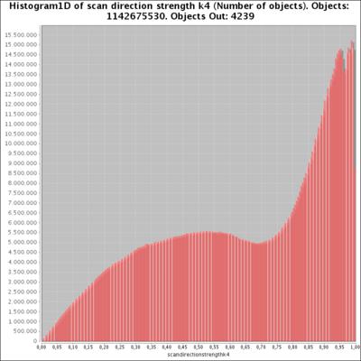
297 Figure 7.55: Histogram of the scan direction mean K1 (larger), mean K2 (larger), mean K3 (larger), and mean K4 (larger). Figure 7.56: HEALPix map in ecliptic coordinates of the mean value of the scan direction mean K1 (larger), mean K2 (larger), mean K3 (larger), mean K4 (larger). Figure 7.57: Histogram of the scan direction strength K1 (larger), strength K2 (larger), strength K3 (larger), strength K4 (larger). Figure 7.58: HEALPix map in ecliptic coordinates of the mean value of the scan direction strength K1 (larger), strength K2 (larger), strength K3 (larger), strength K4 (larger). 295