More Details Fixed point of mapping is point that maps into itself, i.e., x n+1 = x n.

Size: px

Start display at page:

Download "More Details Fixed point of mapping is point that maps into itself, i.e., x n+1 = x n."

Suzan Patterson
5 years ago
Views:

1 More Details Fixed point of mapping is point that maps into itself, i.e., x n+1 = x n. If there are points which, after many iterations of map then fixed point called an attractor. fixed point, If λ < 1, then we have x n+1 apple x n for all. ultimate result of iterations is x = 0. When λ < 1 mapping has 1 fixed point, x = 0, an attractor. Can determine fixed points for given λ by using fixed point condition x n which has solutions x = x(1 x) x = x(1 x)! 1= (1 x)! x =1 1 when x 0 and λ 1. For λ<1 solution is x=0 as stated earlier. Show true: Suppose λ = 1/2 x = 1 2 x(1 x)! x2 + x +0! x(x + 1) = 0! x =0or x = 1(not allowed)

643 as shown Next question is whether fixed points are stable, that is, are they attractors?

2 Geometrically, fixed point = intersection of logistic map function(red curve) with line x n+1 = x n (green curve). Program fixpt.m Fixed point is circle as shown for λ = 0.8 < 1. Intersection (fixed point) is x = 0 as stated. For λ = 2.8 have single fixed point at x = as shown Next question is whether fixed points are stable, that is, are they attractors? To settle question, start with point near fixed point and see if result of iterations converges to fixed point. Can answer question using simple but informative geometrical construction of iteration process near fixed point (program returnmap.m).

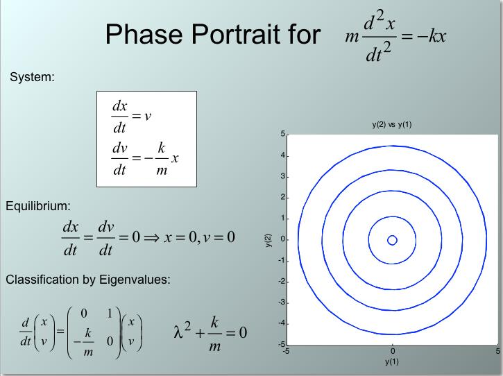
limit or fixed points: points in phase space. Three kinds: attractors, repellers, and saddle points. System moves away from repellers and towards attractors.

3 limit or fixed points: points in phase space. Three kinds: attractors, repellers, and saddle points. System moves away from repellers and towards attractors. Saddle point is both an attractor and a repeller, attracts system in certain regions and repels system in other regions. (see Appendix A - Section for more details). Shown below for 2 cases above. (returnmap.m) For all 0 < λ < 1 fixed point x=0 is stable. Fixed point x 1/λ is stable for 1 < λ < 3. Criterion for stability of fixed point is (1 x fix ) apple 1

or 1 2 1 1 apple 1! 1+ 2 apple 1! +2apple 1! 1 < <3 as expected. Also says no stable fixed points for λ > 3.

set of values (sometimes set will be infinite in number = chaos). For example, look at return map for λ = 3.

4 or apple 1! 1+ 2 apple 1! +2apple 1! 1 < <3 as expected. Also says no stable fixed points for λ > 3. As saw earlier, sequence does not settle down to single value (fixed point) in this case, but oscillates between set of values (sometimes set will be infinite in number = chaos). For example, look at return map for λ = 3.3. Clearly, iteration is alternating between two distinct points. Plot of sequence looks like: (logsen.m) (returnmap.m)

x n+2 = x n or 3 x 2 n(1 x n ) 2 = F (x n ) Plot double map function, single map function (original map function) and line for λ = 2.8.

5 In this region, search for points with higher periodicity, that is, points which return to original value after some number of iterations. For example, period-2 points satisfy x n+2 = x n+1 (1 x n+1 ) = 2 x n (1 x n ) Called double-map function. x n+2 = x n or 3 x 2 n(1 x n ) 2 = F (x n ) Plot double map function, single map function (original map function) and line for λ = 2.8. x n+2 = x n All three curves should intersect at same point (fixed point at 0.643) since already found period-1 fixed point in this case. (quadplot1.m): In case right λ = 3.3, there are three fixed points. Middle one is unstable fixed point of period-1 or single mapping at x = =0.697

Two remaining fixed points of double mapping are stable in range 3 < λ < 3.449.

6 Two remaining fixed points of double mapping are stable in range 3 < λ < Note two points are single pair of period-2 points; calling them and, map takes one into other, i.e, x A = F (x B ) and x B = F (x A ). Another interesting view. x A x B

Transition, as λ raised past critical value (=3), from one stable fixed point to pair of stable period-2 points, known as bifurcation or period doubling.

7 Transition, as λ raised past critical value (=3), from one stable fixed point to pair of stable period-2 points, known as bifurcation or period doubling. period-doubling: change in dynamics where N point attractor replaced by 2N point attractor. Can see another way by plotting time series (sequence of x values) (logmap1.m). Plot below for λ = 0.8 and clearly see map iterate to stable fixed point at x = 0. Next plot below for λ = 1.8 and clearly see map iterate to stable fixed point at x = Next plot(right) for λ = 2.8 and clearly see map iterate to stable fixed point at x = 0.64, in agreement with earlier result.

5 and clearly see map iterate to four stable fixed points = period-4 points. Last plot(right) is in a chaotic regime with no periodicity and no fixed points.

8 Next plot below for λ = 3.3 and clearly see map iterate to two stable fixed points at x = 0.52 and x = 0.80, in agreement with our earlier result = period-2 points. Next plot below for λ = 3.5 and clearly see map iterate to four stable fixed points = period-4 points. Last plot(right) is in a chaotic regime with no periodicity and no fixed points. As λ raised above a second bifurcation occurs (see period-4 points for λ = 3.5 above), that is, pair of stable period-2 point turns into quartet of period-4 points. Such bifurcations occur faster and faster until an infinite number of bifurcations occur at λ =

9 Can see entire structure of logistic map in plot below (logmapall.m). Plot of large number of x values in a sequence for fixed λ value versus λ value. Guess what it will look like? Using this type of plot can see all of other plots. bifurcation diagram: Visual summary of succession of period-doubling produced as control parameter is changed. Clearly, can see the period-1, period-2, period-4, etc regions, bifurcations or period doublings, chaotic regions and many other strange features.

10 Blowup region from to Finally blowup region to

11 Denoting by k the critical value of λ at which bifurcation from stable period-k set of points to stable period-(k+1) set occurs, one finds that = Feigenbaum number. lim k!1 k k 1 k+1 k = This ratio is universal for any map with quadratic maximum and seen in wide range of physical problems. One conclusion can draw from existence of Feigenbaum number is that each bifurcation looks similar up to a magnification factor. This scale invariance or self-similarity plays an important role in transition to or onset of chaos and in structure of strange attractor(discuss shortly). chaos: Behavior of dynamic system that has (a) a very large (possibly infinite) number of attractors and (b) is sensitive to initial conditions.

12 Note from pictures that above shows no periodicity at all. c = attractor set for many (but not all) values of λ For these values of λ quadratic map exhibits chaos and is strange attractor. In region c < <4 there are windows where attractors of small period reappear. Important property of chaotic motion is extreme sensitivity to initial conditions (mentioned earlier). To express sensitivity quantitatively introduce Lyapunov exponent. Lyapunov Number (Liapunov number): value of an exponent, coefficient of time, that reflects rate of departure of dynamic orbits. Measure of sensitivity to initial conditions. Consider two points in phase space separated by distance at time t = 0. If motion is regular (non-chaotic) these two points will remain relatively close, separating at most according to power of time. In chaotic motion two points separate exponentially with time according to d 0 d(t) =d 0 e L t

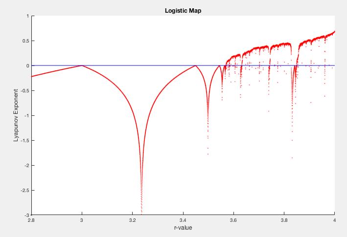
13 Parameter L is Lyapunov exponent. If L is positive motion is chaotic. A zero or negative coefficient indicates non-chaotic motion. There are as many Lyapunov exponents for a particular system as there are variables. Thus, for logistic map there is one Lyapunov exponent. We plot Lyapunov exponent as function of λ, logistic map parameter, below. (See Appendix - Section for more details)

16 Clearly, Lyapunov exponent is negative whenever map is stable and positive whenever map is chaotic. Value of λ is zero when bifurcation occurs and solution becomes unstable. A superstable point occurs where = 1. Can see clearly from plot that when λ goes above zero, there are windows of stability where λ goes negative for a while and period orbits occur amid the chaotic behavior. Relatively wide window just above λ = 3.8 is apparent. Expanding these ideas: Now repeat many ideas have been discussing for better understanding. Bifurcation Diagram So, again, what is a bifurcation? A bifurcation is a period-doubling, a change from an N-point attractor to a 2N-point attractor, which occurs when control parameter is changed. A Bifurcation Diagram is visual summary of succession of period-doublings produced as λ increases.

17 Next figure shows bifurcation diagram of logistic map, λ along x axis. For each value of λ system is first allowed to settle down and then successive values of x are plotted for a large number of iterations. See that for λ < 1, all points are plotted at 0. 0 is the one-point attractor for λ less than 1. For λ between 1 and 3, we still have one-point attractors, but the attracted value of x increases as λ increases, at least to λ = 3. Bifurcations occur at λ = 3, 3.45, 3.54, 3.564, 3.569(approximately), etc, until just beyond 3.57, where the system is chaotic. However, the system is not chaotic for all values of λ greater than 3.57.

Let us zoom in a bit. Notice again that at several values of λ, greater than 3.57, a small number of x values are visited. These regions produce white space in diagram. Look closely at λ = 3.

18 Let us zoom in a bit. Notice again that at several values of λ, greater than 3.57, a small number of x values are visited. These regions produce white space in diagram. Look closely at λ = 3.83 and you will see a three-point attractor. In fact, between 3.57 and 4 there is a rich interleaving of chaos and order. A small change in λ can make a stable system chaotic, and vice versa.

Sensitivity to Initial Conditions Another important feature emerges in chaotic region... To see it, set λ = 3.99 and begin at x 1 =0.3. Next graph shows time series for 48 iterations of logistic map.

19 Sensitivity to Initial Conditions Another important feature emerges in chaotic region... To see it, set λ = 3.99 and begin at x 1 =0.3. Next graph shows time series for 48 iterations of logistic map. logsen0.m Now suppose we alter starting point a bit. Next figure compares time series for x 1 =0.3(open squares) with that for x 1 =0.301 (solid dots).

Two time series stay close for about 10 iterations. But after that, they are pretty much on their own - they diverge from each other. Let us try starting closer together.

20 Two time series stay close for about 10 iterations. But after that, they are pretty much on their own - they diverge from each other. Let us try starting closer together. We next compare starting at 0.3 with starting at This time stay close for longer time, but after 24 iterations they diverge. To see how independent they become, next figure provides scatterplots for two series before and after 24 iterations. Correlation after 24 iterations (right side), is essentially zero. Unreliability has replaced reliability.

21 Have illustrated one symptom of chaos. sensitivity to initial conditions: property of chaotic systems. A dynamic system has sensitivity to initial conditions when very small differences in starting values result in very different behavior. If orbits of nearby starting points diverge, system has sensitivity to initial conditions. A chaotic system is one for which distance between two trajectories or orbits starting from nearby points in its state space diverges over time. Magnitude of divergence increases exponentially in a chaotic system. So what? It is unpredictable, in principle because in order to predict its behavior into future must know its current value precisely. In example, slight difference in sixth decimal place, resulted in prediction failure after 24 iterations. Note that six decimal places far exceeds kind of measuring accuracy typically achieve with natural biological systems.

22 Symptoms of Chaos Beginning to sharpen definition of a chaotic system. First of all, it is a deterministic system. If observe behavior that suspect to be from chaotic system, difficult to distinguish from random behavior sensitive to initial conditions. NOTE: Neither of these symptoms, on their own, are sufficient to identify chaos. Note on technical versus metaphorical uses of terms: Students of chaotic systems have begun to use the (originally mathematical) terms in a metaphorical way. For example, bifurcation, defined here as a period doubling has come to be used to refer to any qualitative change. Even term chaos, has become synonymous, for some with overwhelming anxiety. Metaphors enrich our understanding, and have helped extend nonlinear thinking into new areas. On the other hand, it is important that we are aware of technical/metaphorical difference.

23 Two- and Three-Dimensional Systems First observe distinction between variables(dimensions) and parameters. Consider logistic map x n+1 = x n (1 x n ) Multiply out x n+1 = x n x 2 n replace two λ s with separate parameters, a and b, x n+1 = ax n bx 2 n Now, separate parameters, a and b, govern growth and suppression, but still only one variable x. When have system with two or more variables, 1. its current state is current values of variables 2. treated as point in phase(state) space 3. refer to trajectory or orbit in time

24 Predator-Prey System 2-dimensional dynamic system in which 2 variables grow, but one grows at expense of other. Number of predators is represented by y, number of prey by x. Plot phase space of system - 2-dimensional plot of possible states of system. A = too many predators B = too few prey C = few predators and prey; prey can grow D = Few predators, ample prey Four states are shown. Point A - large number of predators and large number of prey. Drawn from Point A is arrow or vector showing how system would change from that point. Many prey would be eaten, to benefit of predator. Arrow from Point A, therefore, points in direction of smaller value of x and larger value of y.

25 Point B - many predators but few prey. Vector shows that both decrease; predators because too few prey, prey because number of predators is still to prey s disadvantage. Point C, small number of predators - number of prey can increase, still too few prey to sustain predator population. Point D, many prey is advantageous to predators, but number of prey still too small to inhibit prey growth, so numbers increase. Full trajectory (somewhat idealized) is pred2.m

26 Attractor that forms loop called limit cycle. limit cycle: Attractor that is periodic in time, that is, that cycles periodically through an ordered sequence of states. However, system doesn t start outside loop and move into it as final attractor. Any starting state already in final loop. Shown below: loops from four different starting states. Points 1-4 start with same number of prey but different numbers of predators. Look at system over time, that is, as two time series. Figure shows how two variables oscillate, out of phase.

27 Continuous Functions and Differential Equations Changes in discrete variables are expressed with difference equations, such as the logistic map. Changes in continuous variables are expressed with differential equations For example, Predator-prey system is presented as set of two differential equations: dx dt =(a by)x, dy dt =(cx Types of 2-dimensional interactions Other types of 2-dimensional interactions are possible. mutually supportive: larger one gets, faster other grows mutually competitive: each negatively affects other supportive-competitive: Predator-Prey Buckling column system Buckling Column system can be used to discuss psychological phenomena that exhibit oscillations (for example, mood swings, states of consciousness, attitude changes). d)y

28 Model is single, flexible, column that supports mass within horizontally constrained space. If mass sufficiently heavy, column will buckle. 2 dimensions, x representing sideways displacement of column, and y velocity of movement. Shown are two situations, differing in magnitude of mass. Mass on left larger than mass on right. What are the dynamics? Column is elastic, so initial buckle is followed by springy return and bouncing (oscillations). If there is resistance (friction), bouncing will diminish and mass will come to rest. Equations are: dx dt = y, dy dt =(1 m)(ax3 + b + cy)

29 Parameters m and c represent mass and friction respectively. If there is friction (c > 0), and mass is small, column eventually returns to upright position (x = y = 0), illustrated with next two trajectories. For light mass, column comes to rest at single point (attractor) for any starting configuration. With heavy mass, column comes to rest in one of two positions (two-point attractor), again illustrated with two trajectories. Starting at point A, system comes to rest buckled slightly to right, starting at B ends up buckled to left.

30 Now introduce another major concept... Basins of attraction With sufficient mass, buckling column can end up in one of two states, buckled to left or to right. What determines its fate? For given set of parameter values, fate is determined entirely by starting state, initial values of x and y. In fact, each point in phase space classified according to its attractor. Set of points associated with given attractor called attractors basin of attraction. basin of attraction: region in phase space associated with given attractor. Basin of attraction of attractor is set of all (initial) points that go to that attractor.

Basin of attraction for other attractor is unshaded in figure.

31 Shown below - oscillator phase space shaded according to attractor. Average speed < 0 & > 0 Basin of attraction for one of attractors is shaded. Basin of attraction for other attractor is unshaded in figure. Term seperatrix refers to boundary between basins of attraction. For two-point attractor illustrated here - two basins of attraction. (basins.m)

32 Three-dimensional Dynamic Systems - The Lorenz System Lorenz s model of atmospheric dynamics is classic in chaos literature. Model illustrates three-dimensional system. dx dt = a(y x), dy dt = x(b z) y, dz dt = xy cz 3 variables reflecting temperature differences and air movement (details irrelevant). Interested in trajectories of system in phase space. Choose a=10,b=28,c=8/3 - plot part of trajectory starting from (5, 5, 5). Although suggests that trajectory may intersect with earlier passes, in fact never does. Lorenz system shows sensitivity to initial conditions. This is chaos - first strange attractor. Has become icon for chaos.

33 Illustrated dramatically by simulation of Lorenz equations (lorenz0.m and lorenz4.m). Again observe extreme sensitivity to initial conditions. In fact, model was original source of idea of sensitivity to initial conditions! Beasts in Phase space - Limit Points 3 kinds of limit points. Attractors: where system settles down Repellers: point system moves away from Saddle points: an attractor from some regions, repeller in others Examples Attractors: have seen many Repellers: value 0 in Logistic Map Saddle points: point (0,0) in Buckling Column Now return to discussion of the non-linear, damped driven oscillator, which is a real physical system.

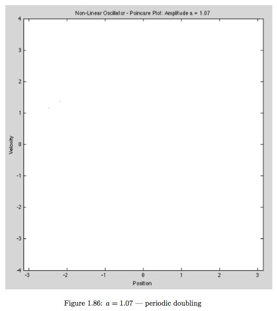
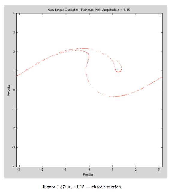
37 The Nonlinear Damped Driven Oscillator(DETAILS) Newtons second law for pendulum (switched variables from x to θ - angle of swinging pendulum) m d2 dt 2 + d dt + sin = cos (!t) First investigate motion of physical system in phase space. Fix some parameters b =1.0 = m = 1 m r g `, ` = pendulum length c =0.5 = m, = damping parameter! = = driving frequency Use as variable (control) parameter (like λ in logistic map) constant a where a = γ/m. In particular, look at a = 0.90! periodic motion a = 1.07! periodic doubling a = 1.15! chaotic motion a = 1.35! periodic motion a = 1.45! periodic doubling a = 1.47! periodic doubling a = 1.50! chaotic motion

38 Run phsp.m to generate phase space plots shown below:

39 Dependence of system motion on amplitude is clearly very complex and sensitive to value.

40 Another way to visualize behavior of systems is via Poincare Plots. Poincare plot is same as using a stroboscope on motion. Flash strobe once every cycle of driving force (frequency = ω). Run phsppoin.m to generate plots shown

41 Alternative picture

48 Poincare plot in this case is attractor with infinite number of points. It is fractal curve (more later) with non-integer dimension. Steady state motion of oscillator at this a and ω is not periodic at all; motion is chaotic. Attractor of this sort is known as strange attractor. Its infinity of points are arranged in strange self-similar (fractal) manner.

49 Finally, make a bifurcation plot for driven oscillator - plot strobe values (from Poincare plot) versus driving amplitude. Thus, two systems, which really do not resemble each other in any way except that they are both nonlinear systems, exhibits very similar behaviors. oscpoinbif.mpg See same structure as in logistic map bifurcation plot. Various periodic, period-doubling and chaotic regions are clear. Critical points are also clear.

50 Zooming in Zoom in on strange attractor. Consider Poincare plot for driven oscillator when a = Looks like figures below. Clear that there is complex structure in strange attractor or fractal at all levels. Dimension of this strange attractor is D = (more later).

54 Only limited by resolution of screen and accuracy of calculation.

55 More images

56 Simulations of chaotic attractor and its Poincare section reveal hierarchical structure that is uncharacteristic of ordinary compact geometrical objects. Chaotic attractor as represented by Poincare sections will be discussed as fractals - mathematical sets of non-integer dimension(strange attractors) - later in these notes. These different magnifications clearly reveal self-similar structure caused by folding and stretching of phase volume. Stretching and folding processes lead to a cascade of scales: attractor consists of an infinite number of layers. Fine structure resembles gross structure property called self-similarity. Properties 1. Trajectory of strange attractor cannot repeat. 2. Nearby trajectories diverge exponentially. 3. Attractor is bounded in phase space. 4. Even though has infinite number of different points, trajectory does not fill phase space

57 Strange attractor is fractal(more later), and fractal dimension(more later) is less than dimension of phase space. Self-Similarity Important (defining) property of fractal is self-similarity, which refers to infinite nesting of structure on all size scales. Strict self-similarity refers to characteristic of form exhibited when substructure resembles superstrucure in the same form. Another example are the Rings of Saturn and the Kirkwood Gaps in the asteroid belt as described in the text.

... it may happen that small differences in the initial conditions produce very great ones in the final phenomena. Henri Poincaré

Chapter 2 Dynamical Systems... it may happen that small differences in the initial conditions produce very great ones in the final phenomena. Henri Poincaré One of the exciting new fields to arise out