Chapitre 4. Transition to chaos. 4.1 One-dimensional maps

Transcription

1 Chapitre 4 Transition to chaos In this chapter we will study how successive bifurcations can lead to chaos when a parameter is tuned. It is not an extensive review : there exists a lot of different manners to transit to chaos, we will just spend some time on the transistions that are rather well known. The understanding of the successive bifurcations leading to chaos is mostly based on the study of one-dimensional maps so that the first section of the chapter will be dedicated to some general useful tools for those kind of studies. The following parts are each dedicated to a transition to chaos : the second part describes the subharmonic cascade, the third one the intermittency phenomenon, and the last part the transition to chaos by quasi-periodicity. The description of each of those transitions will be done using a generic one-dimensional map typical of each road to chaos. The one-dimensional maps that will be studied can have several meanings. They can correspond to a model of a discrete dynamics : for example, the logistic function is used to describe successive generations in population dynamics. But we have also seen that a real, high-dimensional dynamics can be reduced in some conditions to a first return map which can be one-dimensional. Finally, from a pure mathematical point of view, the mere study of a one-dimensional map (as the study of the logistic map by M. J. Feigenbaum) can lead to a very good understanding of the mechanisms underlying chaos by itself. 4.1 One-dimensional maps Let s consider a one-dimensional map f : R R. We study the discrete dynamics given by the successive iterates of the function from an initial point x 0, which is then the initial condition of the time serie defined by : x n+1 = f(x n ). 95

2 96 CHAPITRE 4. TRANSITION TO CHAOS Graphical construction That kind of dynamics can be studied using a graphical construction. We draw the curve y = f(x) and we obtain the successive points using the line y = x : The intersection points of the curve y = f(x) and of the line y = x give the fixed points of the system as they obey to x = f(x ). Those fixed points can be stable or unstable, depending on the behavior of the successive iterates from a point in the vicinity of x Stability of the fixed points Using the tools we have learned in Chapter 1, to determine the stability of a fixed point x we study the iterates stemming from an initial condition x 0 very close to the fixed point x, i.e. x 0 = x + δx 0 with δx 0 x. We can then compute the first approximation of the iterates : x 1 = f(x 0 ) = f(x + δx 0 ) f(x ) + f (x )δx 0 = x + f (x )δx 0 We deduce δx 1 = x 1 x = f (x )δx 0. By iteration, we obtain : δx n = [f (x )] n δx 0 Consequently, and as we have already seen in Chapter 1, if f (x ) < 1, the fixed point is stable and if f (x ) > 1 it is unstable. The stability of the fixed point can thus be deduced graphically by checking the slope of the tangent to the curve in x.

3 4.2. SUBHARMONIC CASCADE Subharmonic cascade This transition is also named a period-doubling cascade : from a periodic behavior of period T, the increase of a parameter leads to a first bifurcation to a new periodic regime of period 2T, then to another one of period 4T, then 8T and so on. We thus observe successive 2 n T periodic regimes whith increasing n until we reach a value of the parameter for which the system becomes chaotic. This transition can be understood by studying the logistic map The logistic map We study the function : f(x) = rx(1 x), where r is a parameter. We will also study this discrete dynamics in the last computer session a Domain of study First, we want the dynamics to be bounded, i.e. that no time series go to infinity. This condition reduces the set of values of x that can be taken as initial conditions. The

4 98 CHAPITRE 4. TRANSITION TO CHAOS curve y = f(x) is a parabola whith a maximum for x = 1/2 and verifying f(0) = 0 and f(1) = 0. As f(1/2) = r/4, if 0 r 4, then for all x [0, 1], f(x) [0, 1]. We will thus consider the dynamics only on the intervall [0, 1] b Fixed points The fixed points are given by : x = rx rx 2 from which we deduce 2 fixed points : x = 0 which is always a fixed point, x = r 1 which exists only when 0 < r 1 < 1, i.e. when r > 1. r r We can see on the following graphs how this new fixed point appears when r increases : c Fixed points stabiity For 0 < r < 1 there is a unique fixed point x = 0. As f (0) = r, 0 < f (0) < 1, the fixed point is stable (see also graphs above).

5 4.2. SUBHARMONIC CASCADE 99 When r exceeds 1, the tangent in 0 becomes greater than 1 and the fixed point 0 becomes unstable. We can observe this change of slope of the curve at the origin on the previous figures. Simultaneously to that destabilization a new intersection of the curve with the line y = x occurs. For 1 < r < 3, the fixed point 0 is now unstable but there is a new fixed point : x = r 1. r ( ) r 1 f = 2 r, r d so that 1 < f (x ) < 1 for 1 < r < 3 and the new fixed point is stable in this range. When r increases above 3 this new fixed point becomes unstable but no new fixed point appears. Consequently, for r > 3 there are two fixed points but the two of them are unstable. Periodic dynamics of the iterate map For 3 < r < , the response of the system is periodic 1. Just after 3, in the permanent regime, the iterates oscillate between two values. This behavior can still be understood by a geometrical construction : To understand this behavior, the function to study is g = f f. Indeed, if we have an oscillation between x 1 and x 2, we have x 2 = f( x 1 ) and x 1 = f( x 2 ), so that x 1 = 1. See Matlab session.

6 100 CHAPITRE 4. TRANSITION TO CHAOS f (f( x 1 )) = g( x 1 ) and x 2 = f (f( x 2 )) = g( x 2 ), which means that x 1 and x 2 are fixed points of g. As a matter of fact, the drawing of the curves y = g(x) before and after r = 3 shows that two new fixed points appear for the function g for r > 3. Those two fixed points appear when the slope of the tangent to the curve y = g(x) in x = r 1 becomes greater than 1. The fixed point x = r 1 becomes then unstable and r r two new stable fixed points appear simultaneously on either sides of x. The bifurcation that occurs is consequently a pitchfork bifurcation. The mathematical study of g can be done. First, we compute the expression of g : To find the fixed points, we write g(x) = rf(x) (1 f(x)) = r [rx(1 x)] [1 rx(1 x)] = r 2 x(1 x) [1 rx(1 x)] x = r 2 x(1 x) [1 rx(1 x)] and then we factorize the polynom r 2 x(1 x) [1 rx(1 x)] x using the fact that r 1 r is a known root. We can then demonstrate that : x 1 = 1 + r (r 1) 2 4 2r which only exists when r 3. and x 2 = 1 + r + (r 1) 2 4 2r To study the stability of those fixed points, we have to calculate g ( x). We have g (x) = f (x)f (f(x)) so that g ( x 1 ) = f ( x 1 )f (f( x 1 )) = f ( x 1 )f ( x 2 ) = g ( x 2 ) Consequently, the two points have necessarily the same stability. The computation gives : g ( x 1,2 ) = r 2 + 2r + 4.

7 4.2. SUBHARMONIC CASCADE 101 The simultaneous destabilization of the the two points happen when g ( x) = 1, at the critical value r = = This destabilization of g is totally similar to the one which has happen to f for r = 3 and is exactly of the same nature. The study of the new periodic regime that arise after the destabilization of x 1 and x 2 can thus be done by studying the iterates of the function h = g g. The drawing the curves of the functions g = f f and h = g g = f f f f for r = 3.56 shows the four new fixed points of h after the destabilization of x 1 and x 2. The scenario we have describe for the moment from r > 3 is the following one : the fixed point x = r 1 of f, which we will consider to correspond to a limit cycle of r period T, becomes unstable at r 1 = 3 through a pitchfork bifurcation which gives rise to a periodic solution characterized by an oscillation between two points x 1 and x 2 (period 2T ). This limit cycle becomes unstable when r leading to a new periodic behavior corresponding to an oscillation between four points (period 4T ).

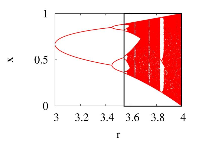
8 102 CHAPITRE 4. TRANSITION TO CHAOS We could pursued this analysis and observe successive pitchfork bifurcations giving each birth to a limit cycle of period twice the previous one. This process continues until a value of r called r : r 1 = 3 r 2 = r 3 = r 4 = r 5 = =... r = Dynamics after r For r > , we can observe either chaotic or periodic dynamics depending on the value of r. In the bifurcation diagram, where are represented the iterates of f in the permanent regime 2, aperiodic responses correspond to vertical lines where the points almost cover segments. We see in the following diagram that there are a lot of values of r for which the response is chaotic but there are also periodic windows, which correspond to values of r where periodicity is recovered. There are an infinity of such windows, we see only the larger ones on the following representations, the largest being the 3T window. 2. See Matlab session.

9 4.2. SUBHARMONIC CASCADE 103

10 104 CHAPITRE 4. TRANSITION TO CHAOS a Lyapounov exponent The chaotic or periodic behaviors can be identified by computing the Lyapounov exponent for each values of r, following the method we saw in the previous chapter : λ = 1 N N ln f (x i ) i=1 For r < r, the Lyapounov exponent is always negative. For r > r, for most of the values of r the Lyaponov exponent is positive, indicating that the regime is chaotic for most of the values of r. In fact, chaotic and periodic domains are closely intertwined : between two values of r for which the behavior is chaotic you can always find a window of values of r for which the behavior is periodic. The Lyapounov exponent for the periodic windows is then negative. Most of the periodic windows are so small that we cannot see them on the figure above because of the lack of resolution of this graph. As for the bifurcation diagram representation, we see only the larger windows.

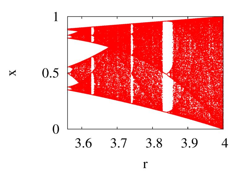
11 4.2. SUBHARMONIC CASCADE b 3T window The study of this window imply to study the function f f f for values of r between 3.8 and 3.9 : The periodic window begins with the simultaneous emergence of 6 new fixed points : 3 stable and 3 unstable. They all appear by pairs of a stable and an unstable point through saddle-node bifurcations. The destabilization of the 3T window occurs through another cascade of period doubling leading to a succession of periodic behaviors : 6T, 12T,..., 3 2 n T. Other periodic windows (5T, 7T,...) can be found in the interval r < r < 4, but their analytical study is more difficult Universality a Qualitative point of view All the phenomenology that we have just studied using the logistic map is shared by a whole class of functions. All the functions that have the same general shape as the logistic function 3 present the same period-doubling cascade leading to a chaotic regime when the parameter is tuned. After r, the order of apparition of the periodic windows is the same. This succession of periodic windows embedded in chaotic regimes is called the universal sequence. For example, we show thereafter a study of the iterates of the function f(x) = r sin(πx), for x [0, 1] and r [0, 1] showing the similarity of the bifurcation diagrams between the logitic map and the sine one. 3. The functions have to be unimodal, i.e., continuous, differentiable, concave and with a maximum. Consequently, all the curves that are bell-shaped.

12 106 CHAPITRE 4. TRANSITION TO CHAOS Quantitative point of view For all those functions, the cascade of period-doubling comes from the fact that the destabilization mechanisms at each bifurcation is the same : only the scales on the axis change as well as the precise form of the function. This similarity can be already seen in the iterates of the logistic function. The following curves show that the parts of the curve of the iterates we need to study to understand

13 4.2. SUBHARMONIC CASCADE 107 each bifurcation have the same shape as the one of the logistic curve but at a smaller scale. In fact, after a proper renormalisation (i.e. a change of the scales of the graphs to superimposed the curves), we obtain from any unimodal function a sequence of unidimensional functions using the iterates f 2n and those sequences all converge to the same universal function. Because of this universal mechanism, the quantitative study of the values of the parameters for which the successive bifurcations occur : r 1, r 2, r 3,..., r n,..., leads to : r n r n 1 r n+1 r δ n n

14 108 CHAPITRE 4. TRANSITION TO CHAOS where δ is a universal constant (Feigenbaum constant), δ = Another scaling law characterizes the change of the size of the successive pitchforks along the vertical axis in the bifurcation diagram. This size corresponds to the distance between the location of the maximum of the initial function (1/2 in the case of the logistic map) and the closest fixed point : The ratio an a n+1 tends toward another universal constant : a n a α, n+1 n with α = This constant is linked to the size factor necessary to rescale the successive curves at each iteration. The limit universal curve is then defined implicitely by : ( x ) f(x) = αf 2. α

15 4.3. INTERMITTENCY Intermittency This kind of transition towards chaos is characterized by the apparition of bursts of irregular behaviors interrupting otherwise regular oscillations. When the parameter is tuned further towards chaos, those bursts are more and more prevalent until a fully chaotic regime is reached Type I intermittency The dynamics is now described by the following one-dimensional map : f(x) = x + ɛ + x 2, where ɛ is a small parameter ( ɛ 1). We study orbits given by the iterates x n+1 = f(x n ). The fixed points are given by : x = x + ɛ + (x ) 2, so that : if ɛ < 0, x = ± ɛ, if ɛ > 0, there are no fixed point. When ɛ < 0, we can determine the stability of the fixed points : f ( ɛ) = ɛ > 1, so that the fixed point + ɛ is unstable f ( ɛ) = 1 2 ɛ < 1, the fixed point ɛ is stable. Consequently, when the parameter ɛ increases from a small negative value to a small positive one, a pair of fixed points, one stable, one unstable, disappears. This scenario corresponds to an inverse saddle-node bifurcation. You can understand from the figures below why a saddle-node bifurcation is also called a tangent bifurcation. When ɛ 0 there are no more fixed points but if ɛ is small enough, the system will spend a lot of time in the region where the function is very close to the line y = x, as shown on the following geometric construction :

16 110 CHAPITRE 4. TRANSITION TO CHAOS When the system is trapped in this region, the observed response is very close to the periodic response which was existing just before the bifurcation, and was corresponding to the stable fixed point ɛ. When the system exits the channel between the curve y = f(x) and the line y = x, the next iterates can take very large values, which correspond to a burst in the temporal response. The system then explores the phase space before to be reinjected at the entrance of the channel where it will again be trapped. The closer to the bifurcation the system is, the longer the time spent in the channel will be. The observed behavior is then quasi-regular oscillations interrupted by irregular bursts. The duration quasi-regular oscillations between the bursts becomes shorter when moving away from the bifurcation Other intermittencies There exists other types of intermittencies but the general behavior : regular oscillations interrupted by bursts of irregular behavior, are common to all those transitions 4. For example, in the type III intermittency, the bursts display a subharmonic behavior and the one-dimensional map associated is : f(x) = (1 + ɛ)x + ax 2 + bx Transition by quasi-periodicity This transition has been proposed by D. Ruelle, F. Takens and S. Newhouse in The mathematical theorem underlying this transition is difficult. Roughly, it says that 3- frequencies quasi-periodicity is not robust : a T 3 torus does not withstand perturbations, however small. Consequently, if a system goes through three successive Hopf bifurcations, there is a very high probability that a strange attractor emerges after the third bifurcation. 4. For more details read the corresponding chapter in L ordre dans le chaos.

17 4.4. TRANSITION BY QUASI-PERIODICITY 111 We will first study a model which gives rise to quasi-periodic but also to frequency locking. Then we will describe how chaos can occur in this system First-return map The one-dimensional map describing this transition is based on a Poincaré section of the torus supporting the 2-frequencies quasi-periodic regime just before the last bifurcation. This section is a closed curve when the regime is indeed quasi-periodic, i.e. when the two frequencies are incommensurable : The one-dimensional variable used to described the system is the angle θ n giving the position of the n th point along the curve, using an arbitrary point as a reference (P 0 in the schematic example). For commodity, a variable which takes its values in the interval [0, 1] is preferred, so that finally the dynamical variable is : φ n = θn. The first return map 2π is the function g such as φ n+1 = g(φ n ). We know that for this kind of dynamics we need to characterize the ratio of the two effective frequencies of the system around the torus. This quantity is given by the winding number : φ n φ 0 σ = lim. n n

18 112 CHAPITRE 4. TRANSITION TO CHAOS When σ is irrational, the system is quasi-periodic. When the system is locked in frequency, σ is a rational p/q, the system is periodic and the Poincaré section displays a finite number of points, q if the section is well chosen. We have then a q-cycle φ 1, φ 2,..., φ q, and g q (φ i ) = φ i + p (mod 1) = φ i. The stability analysis is based on the calculation of : [g q ] (φ) = [ g q 1 g ] (φ) = g (φ) [g q 1] (g(φ)) = g (φ) [g q 2 g ] (g(φ)) = g (φ) g (g(φ)) [g q 2] ( g 2 (φ) ) = g (φ) g (g(φ)) g ( g 2 (φ) ) g ( g q 1 (φ) ) If we apply this formula to any point of a q cycle, we obtain : [g q (φ i )] = g (φ 1) g (φ 2) g (φ q), and the q cycle is stable when q g (φ i ) < 1. i= Arnold s model The archetypal first-return function for the study of the transition to chaos by quasiperiodicity is the following one : φ n+1 = φ n + α β 2π sin(2πφ n) (mod 1), the function is noted g α,β, so that φ n+1 = g α,β (φ n ), and g α,β (φ) = 1 β cos(2πφ). When β = 0, the equation corresponds exactly to the example of trajectories we studied at the beginning of chapter 3 of straight lines of constant slope on the unfold torus. Here the slope of the lines is α and corresponds to the ratio of the two frequencies. The behavior is then periodic or quasi-periodic depending on the value of α. In such an equation (φ n+1 = φ n + α), the two oscillators underlying the dynamics are uncoupled. No locking of the frequencies coming from dynamical reasons is possible. The coupling of the oscillators comes from the β parameter. When β > 0 we will be able to obtain locking or unlocking of the oscillators depending on the value of β for a given value of α.

19 4.4. TRANSITION BY QUASI-PERIODICITY a Frequency locking : Arnold s tongues Case σ = 1 : a winding number σ = 1 corresponds to a a frequency locking 1 : 1 and to a unique point on the Poincaré map. Consequently, it is a fixed point of the map : which leads to the relation φ = φ + α β 2π sin(2πφ ) 2πα β = sin(2πφ ). A solution, and thus a limit cycle, thus exist for 1 < 2πα < 1. Stable cycles verify β 1 β cos(2πφ ) < 1, so that for 0 < β < 1 the obtained limit cycle is always stable. This region of 1 : 1 locking is represented on the following diagram as the hatched area : If α and β are given, the stable fixed point can also be find using a graphical methods for the one-dimensional map : Each of those one-dimensional maps correspond to one of the points on the previous stability diagram. The first one (parameters : blue point on the stability diagram, first return map : blue curve) is the case of a stable fixed point corresponding to the 1 : 1 locking. In the second example (parameters : green point on the stability diagram, first return map :

20 114 CHAPITRE 4. TRANSITION TO CHAOS green curve), fixed points corresponding to φ = g(φ ) still exist but are they all unstable. In the last case (parameters : magenta point on the stability diagram, first return map : magenta curve), no fixed points of the form φ = g(φ ) exists. Case σ = p/q : For other values of σ = p/q, fixed points of the function g q α,β have to be found. For example, for the values of parameter (α = 0.345, β = 0.8) which were our example of a case without 1 : 1 frequency locking, the function g g g has 3 stable fixed points : The domain of existence of this 3 cycle can be studied. For a given value of β we can search for the interval of the values of α for which the fixed points exist and are stable : Studying systematically g 3 α,β, we obtain then a new set of tongues that we can add to the stability diagram.

21 4.4. TRANSITION BY QUASI-PERIODICITY 115 Repeating this study we obtain domains of frequency locking, called Arnold s tongues, that we can gather on a diagram. For a given 0 < β < 1, we have intervals of frequency locking separated by domains of quasi-periodicity. Figure 4.1 Figure from V. Croquette course http: // If we represent the winding number σ as a function of α, the graph looks like a staircase, called a devil s staircase, formed by horizontal plateaus corresponding to the locking domains. When β increases, the width of the stairs widened and the locking domains are wider and wider. At β = 1, the tongues are touching each other and the unlocked domains of quasi-periodicity form a set of points almost empty. The staircase is said to be complete, the sum of the width of all the stairs is equal to 1. Figure 4.2 Arnold s tongues, figure from V. Croquette course b Transition to chaos When β > 1, the tongues corresponding to frequency locking in the (α, β) plane overlap. Moreover, if we go back to the study of the one-dimensional map, we observe that the map is not any more inversible for β > 1 :

22 116 CHAPITRE 4. TRANSITION TO CHAOS The non-inversibility is the fact that several φ n+1 can have different antecedents. It appears when the curve is not monotoneous anymore. As g α,β (φ) = 1 β cos(2πφ), the noninversibility appears when the derivative can change sign, i.e. for β > 1. From the Poincaré section point of view it corresponds to a folding of the closed curve, which is an indication of the destruction of the torus. Figures from the book Deterministic Chaos, W.G Schuster and W. Just.

23 4.4. TRANSITION BY QUASI-PERIODICITY 117 In the domain β > 1, we can then observe chaos when the torus is destroyed. Still, some regions of locking persist for some values of the parameters, but outside those regions we observe chaos. Their is a close imbrication of chaotic domains and periodic domains in the parameter space. As for the other studied routes towards chaos, the main features of the transitions does not depend of the precise form of the considered map but of some generic properties of the first return map. Conclusion In this chapter we studied very briefly some routes towards chaos. What is important to note is that all those transitions depend only on a few general properties of the function describing the dynamics of the system. When a first-return map is closed to one of the model maps that have been presented in this chapter, the transition to chaos will be of the type of the corresponding model. This universality explain why those routes have been observed in very different systems. Much more transitions to chaos exist and most of them are far from being understood as well as the ones described here. Bibliography In English : Deterministic Chaos, An Introduction, H. G. Schuster and W. Just In French : L ordre dans le chaos, P. Bergé, Y. Pomeau, C. Vidal Cours DEA de V. Croquette, croquette/index.html